
Markowitz Mean-Variance Portfolio Optimization with Predictive Stock Selection Using Machine Learning


School of Management Technology, Sirindhorn International Institute of Technology, Thammasat University, Pathum Thani 12120, Thailand
*
Author to whom correspondence should be addressed.
Int. J. Financial Stud. 2022, 10(3), 64; https://0-doi-org.brum.beds.ac.uk/10.3390/ijfs10030064
Submission received: 1 July 2022
/
Revised: 2 August 2022
/
Accepted: 2 August 2022
/
Published: 8 August 2022
(This article belongs to the Special Issue Asset Pricing, Investments and Portfolio Management)
Abstract
:With the advances in time-series prediction, several recent developments in machine learning have shown that integrating prediction methods into portfolio selection is a great opportunity. In this paper, we propose a novel approach to portfolio formation strategy based on a hybrid machine learning model that combines convolutional neural network (CNN) and bidirectional long short-term memory (BiLSTM) with robust input features obtained from Huber’s location for stock prediction and the Markowitz mean-variance (MV) model for optimal portfolio construction. Specifically, this study first applies a prediction method for stock preselection to ensure high-quality stock inputs for portfolio formation. Then, the predicted results are integrated into the MV model. To comprehensively demonstrate the superiority of the proposed model, we used two portfolio models, the MV model and the equal-weight portfolio (1/N) model, with LSTM, BiLSTM, and CNN-BiLSTM, and employed them as benchmarks. Between January 2015 and December 2020, historical data from the Stock Exchange of Thailand 50 Index (SET50) were collected for the study. The experiment shows that integrating preselection of stocks can improve MV performance, and the results of the proposed method show that they outperform comparison models in terms of Sharpe ratio, mean return, and risk.
1. Introduction
Portfolio management is an analytical process of selecting and allocating a group of investment assets in which the portion of allocated investment is persistently changed to optimize expected return and risk tolerance (Markowitz 1952). The Markowitz mean-variance (MV) model, first developed in 1952, is the foundation of portfolio theory, which is extensively used and recognized in portfolio management (Sharpe and Markowitz 1989). However, based on the classical MV model, there are two main issues of concern for practical application. The first is that the MV relies on the expected return and risk of asset inputs to produce optimal portfolios for each level of expected return and risk (Beheshti 2018). As a result, by selecting good assets to put into the optimization process, the MV model may achieve improved performance (Mitra Thakur et al. 2018). Another issue is that many high-risk assets often return a large number of small-scale weights in the optimal portfolio, which makes them difficult to implement, particularly for individual investors (Ben Salah et al. 2018; Ortiz et al. 2021; Huang et al. 2021).
In recent years, machine learning has been proven to be advantageous in quantitative finance (Dixon et al. 2020); portfolio optimization is one of the most interesting problems in this regard. Normally, the MV model relies on historical data to generate the optimal portfolio and can only show the optimal portfolio as far as the data input. Therefore, a number of researchers have been applying machine learning for predicting return and volatility in the future (Henrique et al. 2019). Investors in the financial market must evaluate a variety of factors and perspectives to maximize their investment earnings (Rahiminezhad Galankashi et al. 2020). In this regard, including stock price prediction methods in portfolio optimization would be advantageous and profitable for investors (Kolm et al. 2014). Financial time-series prediction has long been a difficult field of study since financial market fluctuations are inherently unstable, complex, and dynamic (Paiva et al. 2019). However, several related studies claim that there is a pattern of asset price movement in financial time-series data and that this pattern may be used to forecast financial time-series data to some extent (Wan et al. 2020; Wang et al. 2020).
The main purpose of this study is to develop a portfolio-formation approach for individual investors in which a hybrid machine learning model that combines convolutional neural network and bidirectional long short-term memory with robust input features (R-CNN-BiLSTM) is applied to predict future stock closing prices before using the MV model to form the optimal portfolio. In this regard, this study has two main contributions that fill the gap in the existing literature. Firstly, this study proposes a novel approach for portfolio formation that combines R-CNN-BiLSTM and MV (R-CNN-BiLSTM+MV1). This method, which is suitable for capturing the pattern in financial time-series data, leverages robust input instead of direct stock closing price for machine learning training. Three LSTM-based machine learning models (i.e., LSTM, BiLSTM, and CNN-BiLSTM) are used as comparison models in this experiment to compare the results with the R-CNN-BiLSTM model in terms of prediction accuracy to illustrate the superiority of the proposed method. Second, the method includes a stock selection process to ensure the quality of stock inputs, in which stocks with higher potential returns are selected as candidates before constructing different sizes of optimal portfolios using the MV model to determine the appropriate number of stocks in the optimal portfolio that provide the best return and risk for individual investors.
The remainder of the paper is organized as follows. In Section 2, reviews of some existing studies are discussed relating to stock prediction and portfolio optimization, as well as empirical works that employ traditional statistics and machine learning methods to solve problems in relation to stock prediction and selection. Section 3 briefly explains the underlying knowledge used in this study. Section 4 presents the detailed experimental process. Section 5 reports the experimental results. Finally, Section 6 addresses the work’s key findings, theory implementations, and limitations.
2. Literature Review
Many studies have been performed on the process of stock selection and portfolio optimization using various methods. Lozza et al. (2011) proposed the ex-post comparison of asset preselection strategies using the joint Markovian behavior of the returns in relation to market stochastic bounds to deal with large-scale portfolio selection with approximately 10,000 stocks from 14 different stock markets and discovered that Markovian strategies outperformed the classical approach based on maximizing Sharpe ratio. Huang (2012) proposed a stock selection model using the support-vector machine (SVR) and genetic algorithms (GA). This model applies SVR to predict each stock’s future performance, with GA utilized to optimize model parameters and input characteristics. The highest-ranked stocks are then weighted equally to build the portfolio. The experimental results show that the investment performance of the proposed model is better than the benchmarks. Nguyen (2014) proposed a risk-measurement method for large-scale datasets that includes a stock-preselecting procedure to remove low-diversification stocks before optimization using the Sharpe ratio, Stutzer performance index, and the Omega measure. The experimental results showed that the preselection process improved the performance and diversification of the proposed portfolio. Rather et al. (2015) proposed a novel robust hybrid model for stock return prediction. The model consists of two linear models, the autoregressive moving average and the exponential smoothing models, and a non-linear model, a recurrent neural network (RNN). The proposed model combined the results of these three prediction-based methods with the objective to improve the accuracy of the model prediction. The optimization model was then used to generate the model’s ideal weight using GA. The proposed hybrid prediction model outperformed the RNN model in terms of the prediction accuracy. Le Caillec et al. (2017) integrated several indicators for stock selection using analysis performance evaluation and a behavioral uncertainty framework of human bias to calculate the cumulative return (CR) of the portfolio. The combined methods, one probabilistic and one possibilistic, focused on discriminating the common use of multiple technical indicators (TI) to preselect stocks based on the probabilistic framework. Experiments showed that the proposed model could raise portfolio performance. Fischer and Krauss (2018) implemented the LSTM neural network to predict the directional movement of the constituent stocks of the S&P 500 from 1992 to 2015. The study found that the portfolio based on the LSTM outperformed the other machine learning models without a memory function (i.e., RF, DNN, and LR).
These models only apply simple portfolio construction methods that ignore individual stock risk, such as the equal-weight method, which resulted in a portfolio with unbalanced risk and expected return. As a result, they are not suitable for individual investors in practice. Due to the shortcomings of the models, some researchers have adopted the MV model and used a quantitative method to improve investment decisions.
Tu and Zhou (2010) incorporated Bayesian priors with economic objective functions in the MV model in which the priors were imposed on the solution rather than primitive parameters. The study used the monthly return on a Fama-French 25 size from January 1965 to December 2004 and book-to-market portfolio. The results show that portfolio strategies using objective-based priors outperformed the standard portfolio allocation. Brown and Smith (2011) studied some heuristic trading strategies in portfolio optimization and developed a dual approach to examine the quality of the heuristics. The approach considered several utility functions, i.e., transaction costs, constraint sets, and models of returns. Most heuristic models performed very close to the optimal solution in the experiment, indicating that the heuristics model could capture the tradeoff between improving the position of assets and reducing the transaction costs. Li et al. (2015) proposed a specific portfolio selection approach using background risk. The study compared a probabilistic portfolio model with background risk to a probabilistic portfolio without background risk. The experiment indicated that when the expected return is the same, the variance of the background risk is larger than the one without risk. Bodnar et al. (2017) analyzed the weights in the optimal portfolio using the Bayesian framework. This approach enabled investor’s beliefs to be incorporated into portfolio selection. The study derived explicit formulas for the posterior distributions of linear combinations of global minimum variance (GMV) using different priors for the return of assets, specifically, the non-informative (diffuse) and the informative (conjugate and hierarchical) priors. Then, the prior is suggested directly for the weights of the portfolio. The numerical study results showed that the studies performed well for the suggested prior. Katsikis et al. (2021) presented an online approach for time-varying financial problems while removing the limitations of static methods. The study found that time-varying mean-variance portfolio selection with transaction costs and a cardinality constraint (TV-MVPSTC-CC) can be made more realistic by using technical analysis to generate the expected return of a portfolio. Additionally, a beetle antennae search (BAS) was implemented to automatically adjust the parameters, which results in dramatically improved computationally efficacy. The results demonstrated that BAS more is suitable than the Fa, Ga, and De algorithms for portfolio configurations in real-world data. Khan et al. (2021) developed a meta-heuristic optimization called quantum beetle antennae search (QBAS) and incorporated it into portfolio selection to generate the optimal portfolio. The study applied QBAS on real-world data from the Shanghai Stock Exchange 50 Index (SSE50) and compared the performance to conventional algorithms (i.e., particle swarm optimization (PSO), genetic algorithm (GA), and beetle antennae search (BAS)). The experimental results showed that QBAS outperformed other algorithms in terms of time-consumption, especially for extensive data. Although this method is neither computationally expensive nor time-consuming, the optimal portfolio still relies on historical data. Khan et al. (2022) proposed a meta-heuristic algorithm called non-linear activated beetle antenna search (NABAS) and formulated a tax-aware portfolio, which is a non-convex problem where conventional algorithms can be stuck in local minima. The study used data from 20 companies in National Association of Securities Dealers Automatic Quotation System (NASDAQ) to compare its performance with that of BAS, PSO, and GA. The results indicated that the performance of NABAS is comparable to BAS, PSO, and GA for convex problems and is apparently better for non-convex problems, as the method is immune to local minima. Khan et al. (2020) proposed a non-convex method for portfolio selection using BAS. The method takes cardinality and transaction costs into consideration to enhance the classical Markowitz and reformulates it as an unconstrained optimization problem before solving the problem using BAS. Additionally, the study compared the performance of the proposed method to that of PS, PSO, and GA. The experimental results showed that BAS’s performance was six times faster than others’ performance in the worst case and twenty-five times faster than others’ performance, in the best case with comparable accuracy.
These models show us more reasonable and balanced portfolios using the MV model, in which some models are very computationally efficient. However, they are not effective in dealing with complex financial time-series data and are not able to accurately predict potential outcomes in the future, which leads to a difficult situation of asset preselection, where only applying complex methods without the selection of high-quality asset inputs before the optimization is not sustainable. In this regard, several scholars have focused more on incorporating machine learning and deep learning to capture the complex financial time-series data rather than improving the optimization model.
Alizadeh et al. (2010) developed a portfolio optimization model using an adaptive neural fuzzy inference system to predict portfolio returns and an index of variance for risk assessment. The results of the experiment show that this portfolio optimization model outperforms the MV, neural network, and Sugeno–Yasukawa models. This research tells us that the combination of artificial intelligence techniques with modern portfolio optimization can produce better performance than any single trading investment model. Paiva et al. (2019) proposed a single decision-making model for day-trading stock market investments, which was developed using a composite approach of SVM and MV models for portfolio selection. The proposed model is compared with two other models, namely SVM+1/N and Random+MV. An experimental evaluation based on Ibovespa’s stock market assets shows that the proposed model works best. Wang et al. (2020) proposed a portfolio formation method consisting of LSTM networks and an MV model. The LSTM is applied to capture stock price patterns using a variety of technical indicators as input variables, such as Relative Strength Index (RSI), Momentum Index (MOM), and True Range (TR). The MV model was used to generate optimal portfolios with different numbers of assets between five and ten candidates before benchmarking with other combined machine learning and MV models. The experimental results showed that the proposed method, which is LSTM+MV, outperformed other models, especially when the number of stocks in the portfolio is ten. Ta et al. (2020) built the portfolio using LSTM neural network and three portfolio optimization techniques, namely the equal weight method, Monte Carlo simulation, and the MV model. In addition, they applied linear regression and SVM for comparison in the stock selection process. The test results show that the LSTM neural network outperforms linear regression and SVM in terms of prediction accuracy, and its built portfolio outperforms that of others. Chen et al. (2021) developed a novel portfolio construction in which a hybrid machine learning-based model, eXtreme Gradient Boosting (XGBoost) with an improved firefly algorithm (IFA), was applied to predict the future stock price, and then the MV model was employed to select sets of a different number of stocks with higher predicted returns into optimal portfolios. Empirical results showed that the results of the proposed model were superior to other results of benchmark models, especially when the portfolio contained seven stocks.
These models apply different machine learning and deep learning methods for stock selection, then develop portfolio optimization models with the selected stocks for trading investments. These methods point us in a promising direction to build portfolio models in practice. It is obvious that several related studies mainly focus on how to improve the quality of assets input before optimization rather than to improve Markowitz’s optimization model. As a result, in order to advance research on portfolio optimization, this study attempts to follow logical procedures and adapt the original MV model.
3. Background Knowledge
3.1. Mean-Variance Optimization
Markowitz (1952) proposed the mean-variance (MV) model and was awarded the Noble Prize in Economics in 1990. The MV model made use of mean and variance, which are calculated from historical asset prices to quantify the expected return and risk of the generated portfolio. The MV model assumes that the investor would like to either maximize the expected return for a given level of risk or minimize risk for a given return (Kolm et al. 2014). However, in this study, we only show the optimization with minimum variance. The MV model is described as follows:
where N represents the total number of assets, which indicates the dimensionality of the optimization in the portfolio; is the weight of each i asset in the portfolio to be optimized; stands for the variance of the portfolio which generally refers to portfolio risk; is the covariance of return between asset i and j; is the expected or target return; and is the average return on an individual asset i.
3.2. CNN
A convolutional neural network (CNN) is a kind of deep learning model for processing grid pattern data, such as image processing and natural language processing. CNN can be applied to predict time-series data (Sadouk 2019). CNN can significantly improve the quality of the learning models by reducing the number of parameters. CNN is mainly composed of three types of layers: a convolution layer, a pooling layer, and a fully connected layer (Albawi et al. 2017). The first two layers, the convolution layer and the pooling layer, execute feature extraction, while the last layer, the fully connected layer, directs the extracted features into output (Milošević and Racković 2019).
3.3. LSTM
Long short-term memory (LSTM) was proposed by Hochreiter and Schmidhuber (Hochreiter and Schmidhuber 1997). The model is a class of RNN but has a function of memory, which enables LSTM to retrain data over a long period of time compared to RNN (Fischer and Krauss 2018). The LSTM model filtrates information that enters through gate structures composed of an input gate, a forget gate, and an output gate to improve and maintain memory cells. LSTM is particularly popular in the field of financial time-series prediction, since the model can effectively handle the redundancy in historical data (Gao et al. 2021). The operation equation of LSTM is as follows:
Forget gate:
Input gate:
Output gate:
where , , and refer to forget gate, input gate, and output gate, respectively; w represents the weight of the matrix; , , and indicate the bias of the forget gate, input gate, and output gate, respectively; stands for sigmoid function; and denote the input and current output at time t, respectively; is the value from the input gate at time t; and the hyperbolic function (tangent) is represented by tanh.
3.4. BiLSTM
Bidirectional long short-term memory (BiLSTM) is an improved version of LSTM with the ability to access both forward and backward directions of the input feature (Dong et al. 2014). The key difference between BiLSTM and LSTM is that it uses two hidden layers. BiLSTM was shown to be better compared to LSTM in terms of time-series data prediction (Siami-Namini et al. 2019). The hidden layer output of BiLSTM has the activation function for both forward and backward. The BiLSTM equations (Yang and Wang 2022) are described as follows:
where σ stands for the activation function of the model; is the weight of the matrix; is the weight of input (x) to the hidden layer (h); indicates the hidden layer input; and denotes the bias of the respective gates (x). The output is carried out by updating forward and backward structures.
3.5. Robust Statistics
In real-world applications, data collection often includes some atypical observations that deviate from the majority or bulk of the data, in which these observations are referred to as outliers, especially in financial time-series data. For example, for stock prices, the outliers deviate from the general pattern of the data. Therefore, it is very difficult to predict future stock prices. To overcome these limitations, this study uses robust statistics theory (Maronna et al. 2019) to estimate the appropriate dataset to be used in the training process of machine learning.
3.5.1. The Classical Robust Location Estimator
The sample mean and median are considered location estimators of the distribution of the data. The main difference is that the sample mean is not robust to extreme outliers. For example, the closing price of a certain stock in a week falls immediately for unexpected reasons. For example, provided that historical closing prices of a certain stock are {243, 190, 150, 80, 56, 28, 142}, in this case, the sample mean is 127, which is not considered a good location estimator for these observations. Next, the median of the sample is 150, which is a robust location estimator of the data. However, if the distribution of the data is considered approximately normal, the sample mean would then be considered a better estimator than the sample median. The robust location estimator is a combination of these two classical estimators. To put it precisely, when there are extreme outliers in the observations, the robust estimator approximates the sample median. On the other hand, the estimated location approximates the sample mean.
3.5.2. Huber’s Location Estimator
Huber (1964) proposed a good combination of mean and median, called the robust location estimator or M-estimator of a location, which can be described as follows:
where is a robust location estimator of the observation; is the variable of observation I; stands for the error function. The robust location is a parameter that minimizes the function to ensure that the parameter provides the minimum error between the location estimator and all observations. Several methods have been proposed (Maronna et al. 2006) to find the local minimum of the function such as the maximum likelihood estimator (MLE). In this paper, we use a numerical method, the Newton–Raphson method, to find the robust location estimator.
The Newton–Raphson method is an iterative method for solving non-linear equations. To solve the equation , is set to be linearized for each iteration. In a location M-estimator, it is necessary to solve the equation for . The iterations are defined as follows:
where is the value of the location estimator at iteration m. The of observation is defined by the following function with respect to a given positive constant of as follows:
if is bounded, its derivative tends to be zero at infinity (Hampel et al. 2011). If approaches infinity, then the is the mean. On the other hand, if approaches zero, then the acts as the median. In this paper, we use in our proposed method. This value is similar to that used by Fox and Weisberg (2019).
4. Experimental Process
4.1. Data Preparation
One of the greatest challenges in stock prediction is to capture the pattern of financial time-series data between the past and future (Wang et al. 2020). Hence, it is easier to predict stable stocks than volatile stocks. The Stock Exchange of Thailand SET 50 index (SET50) consists of the topmost 50 large-capitalization companies in the stock market of Thailand, which comprehensively reflect the overall situation of the stock market in Thailand. In this study, the historical data of the stocks in SET50 are considered as the experimental data set according to characteristics of stability and large scale of the stocks. Additionally, some related studies have been conducted by selecting 21–49 stocks as the experimental data set. Wang et al. (2020) randomly select 21 stocks from FTSE100 as the sample for machine learning prediction process before optimization. Chen et al. (2021) randomly chose 24 stocks from SSE50 as candidate assets in stock prediction process before forming a portfolio. Ma et al. (2021) employed 49 stocks from SSE100 as a dataset for stock prediction using machine learning before constructing a portfolio. Additionally, numerous researchers agree on holding around 10 different stocks in the portfolio. For instance, Soeryana et al. (2017) chose five different stocks in the optimal portfolio. Abrami and Marsoem (2021) constructed an eight-asset portfolio. Therefore, our study randomly selected 25 stocks that have been fully trading between 1 January 2015 and 30 December 2020 covering 1462 trading days from the SET50 index and used closing price as the experimental data set, which is sufficiently large for individual investors to build a portfolio (Zaimovic et al. 2021). The names of these stocks are “Airport of Thailand” (AOT), “Bangkok Dusit Medical Services” (BDMS), “Bangkok Expressway and Metro” (BEM), “Berli Jucker” (BJC), “BTS Group Holdings” (BTS), “CP ALL” (CPALL), “Central Pattana” (CPN), “Delta Electronics Thailand” (DELTA), “Total Access Communication” (DTAC), “Energy Absolute” (EA), “Siam Global House” (GLOBAL), “Intouch Holdings” (INTUCH), “IRPC” (IRPC), “Indorama Ventures” (IVL), “KCE Electronics” (KCE), “Krungthai Card” (KTC), “Land & Houses Public” (LH), “Minor International” (MINT), “Muangthai Capital” (MTC), “Petroleum Authority of Thailand” (PTT), “PTT Exploration and Production” (PTTEP), “PTT Global Chemical” (PTTGC), “Ratch Group” (RATCH), “Srisawad Corporation” (SAWAD), and “The Siam Cement” (SCC).
Table 1 presents summary statistics of close prices for the 25 stocks. The stocks with the highest and lowest returns are clearly Delta and IRPC, while the stocks with the highest and lowest standard deviation are SCC and LH, respectively.
4.1.1. Architecture of R-CNN-BiLSTM
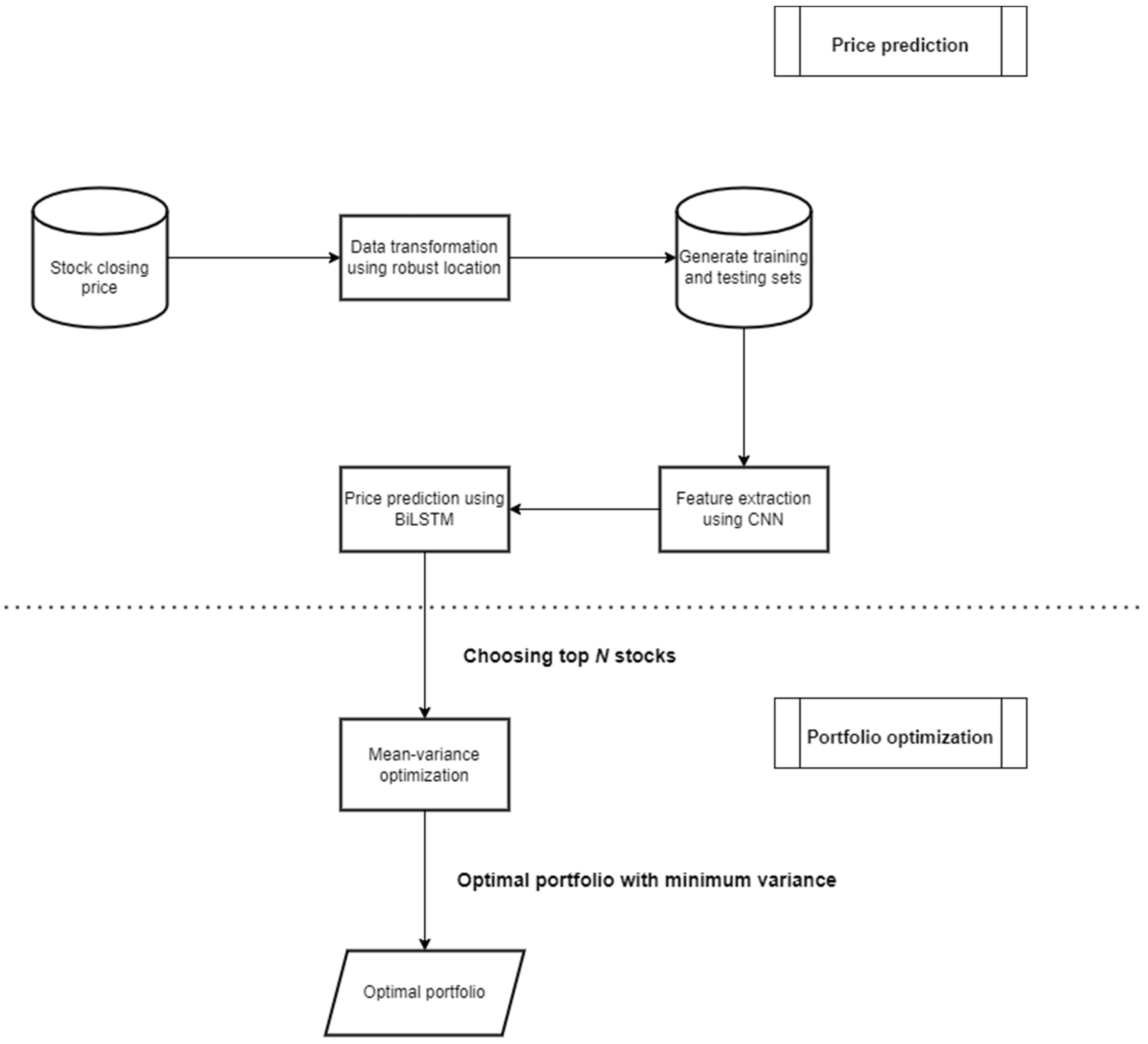
This study proposes a hybrid R-CNN-BiLSTM model to improve the accuracy of the prediction. The detailed process of the proposed model is presented in Figure 1.
The proposed model consists of three parts: data transformation, feature extraction, and price prediction.
First, the data transformation component converts the stock closing prices into the robust domain, which is the non-noisy version of the data. In this study, the direct stock closing price data are not suitable for machine learning training due to high standard deviations. Therefore, we need to transform the data to make them more suitable for the training process. Stock closing prices are divided into a small time-series size of 4 days, the so-called lag time. The lag times overlap 1 day with each other. The Huber’s location estimator of each lag time is calculated using Equations (14) and (15).
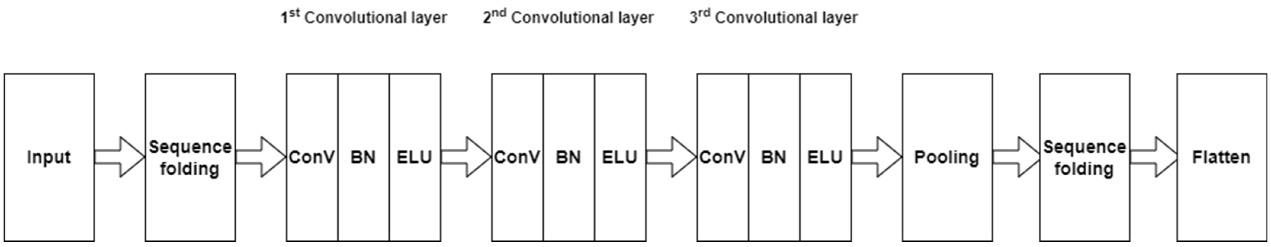
Second, the feature extraction is performed using a CNN network. CNN has the ability to identify important factors in the data, which are called “features”. The purpose of this step is to preserve the historical data in the time-series data and feed them into BiLSTM. Therefore, the input data is converted by performing convolutional operations on the time steps of the time-series data using a sequence folding layer. In the next step, the two-dimensional convolutional layer is used to extract the data features. The filtering size of the first convolutional layer is , and the stride parameter is set to {}, where a is a vertical step size and b is a horizontal step size. The first convolutional layer is followed by Batch Normalize (BN), which normalizes a mini batch of data over all data points to speed up the training process of the CNN. In our model, The Exponential Linear Unit (ELU) is used as the activation function. This function performs the identity operation on positive inputs and exponential nonlinearity on negative inputs. The filtering size of the second and third convolutional layers increases to and , respectively. The next layer is the pooling layer. It performs down-sampling by dividing the data into sub-regions and then calculating the maximum of each region. The sequence structure of the input is restored using the sequence unfolding layer. Finally, the spatial dimensions of data are collapsed with the flatten layer. The overview of the proposed framework of the CNN model is shown in Figure 2.
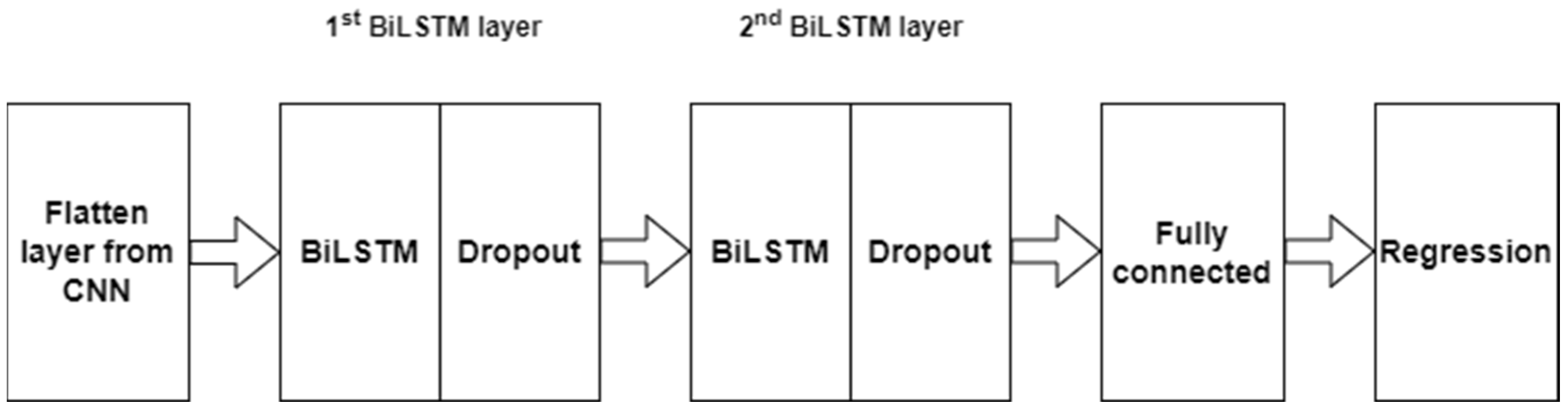
Finally, the price prediction using BiLSTM is performed. The flattened data from the CNN are used as the input of BiLSTM. The input size of the first BiLSTM layer is , and the number of hidden units is 128. Tanh is used as the state activation function and Sigmoid as a gate activation function. To prevent the network from overfitting, we put the dropout layer next to BiLSTM layer. Its operation changes the underlying network architecture between interactions by randomly setting input elements to zero with uniform probability. For the second BiLSTM layer, we decrease the input size and the number of hidden units to 256 and 16, respectively. The last two layers are fully connected, and regression layers are the standard of CNN architecture. The BiLSTM framework is shown in Figure 3.
4.1.2. Process of Training and Testing
One of the most important factors that determine the success of machine learning is the process of training and testing. In this study, we divided the close price of each chosen stock into training and testing sets according to the ratio of 80:20. Therefore, the first 1201 days of data are used in the training process, and the last 262 days are used as the testing set.
4.1.3. Hyperparameter Setting
The training dataset is passed to the proposed model for training. In this step, the various hyperparameters of the neural network are specified. These include the number of hidden layers, the number of epochs, and the size of batch inputs. Finding the optimal hyperparameters is still a major challenge in the field of deep learning. In this study, hyperparameters are set manually by trial and error with the selection of best parameters from the experiment. The following is a detailed description of the hyperparameters and their value settings.
- The number of epochs: An epoch is one round of full training. In our experiments, we set the number of epochs to 100 and performed our training. After training, we found that all training stops at a maximum of 100 to 120 epochs. Therefore, 100 is selected as the value for this hyperparameter.
- The number of hidden layers: This is the number of layers between input and output layers. For the CNN network, we set the hidden convolutional layer counts to 100, 100, and 50. In the BiLSTM network, we set these numbers to 128 and 16.
- Learning rate: This value is set for the accurate model convergence of the model in prediction. In our experiment, we set a learning rate to 0.0001. Many researchers recommend using a learning value lower than 0.01 (Hastie et al. 2017).
- Optimizer: This is the optimization function used to obtain the best results. In our work, we use the Adam optimizer, as it works well for LSTM based networks.
- Loss function: Mean Squared Error (MSE) was used as the loss function. Our implementation was written using MATLAB with GPU computing.
4.1.4. Stock Selection
Once all the stock prices are successfully predicted, high-quality stocks are selected to perform in the optimization process one by one by ranking them in descending order based on the expected (average) return. The predicted stock price is used to calculate the stock return using Equation (17).
where is the return of the stock at time , while is the predicted stock price at time and is the predicted stock price at time .
As a result, we select the top () number of stocks with a higher potential return according to the ranking order. Only the selected stocks are qualified for constructing the portfolio in the next stage. The MV model is used in this process to build the optimal portfolio with different proportions of asset allocation based on the qualified stocks. The optimization process is performed using the MS Excel solver in which the minimum variance is set as the objective function, and the weight of each asset is adjusted using the Excel solver. Consequently, each of the optimal portfolios with the lowest variance is found and used for analysis.
4.2. Benchmark with Comparison Models
To comprehensively benchmark the R-CNN-BiLSTM+MV, three representative machine learning models (LSTM, BiLSTM, and CNN-BiLSTM) and two portfolio models, the MV model and equal-weight portfolio (1/N) model, were employed. The hyperparameters are set as in the proposed model, and the following models are comparison models.
4.2.1. Comparison Model 1: R-CNN-BiLSTM+1/N
The prediction process to select stocks for the optimization of this model is the same as R-CNN-BiLSTM. The only difference is that all the weights of selected stocks are equally distributed. Specifically, in the first stage, R-CNN-BiLSTM is used to predict future stock close prices, and then the top N stocks ranking with a higher predicted return are selected and weighted equally in the portfolio. The objective of this comparison model is to see the performance of the MV model when the same set of stocks are chosen.
4.2.2. Comparison Model 2: Machine Learning+MV and Machine Learning+1/N
The objective of this comparison model is to investigate whether the different prediction models affect the optimal portfolio. Specifically, the stock closing prices are predicted using LSTM, BiLSTM, and CNN-BiLSTM, and the stocks with the higher predicted return are chosen to put into either the MV model or the 1/N model. In addition, the number of N stocks is consistent with R-CNN-BiLSTM+MV. Note that the hyperparameters are set as the proposed model.
4.2.3. Comparison Model 3: Random+MV and Random+1/N
This comparison model is totally different from the previous models in terms of stock selection. Specifically, in the first stage, the stock prediction is carried out randomly without relying on any machine learning models. The stocks to be processed in the portfolio optimization using either the MV model or the 1/N model are selected randomly from all the samples in the second stage. The main objective of this strategy is to examine the necessity of stock selection using machine learning.
5. Experimental Results
This section first presents the prediction performance of the LSTM, BiLSTM, CNN-BiLSTM, and R-CNN-BiLSTM models. In the following, this study constructs different sizes of portfolios using the classical MV model to compare the prediction result of different machine learning models without a transaction fee.
5.1. Prediction Performance Results
5.1.1. Machine Learning Metrics
In this section, the predictive accuracy of machine learning models is evaluated by three criteria, mean absolute error (MAE), mean square error (MSE), and mean absolute percentage error (SMAPE), as they are extensively used as performance metrics (Jierula et al. 2021; Singh et al. 2021). These measures are described as follows:
where refers to the predicted price, represents the true value, and n indicates the total number of stocks used in the experiment.
5.1.2. Performance of the Prediction
Table 2 and Table 3 present the results of each model that has been applied in accordance with the performance metrics employed. According to the two tables, it can be clearly seen that the R-CNN-BiLSTM model provides most of the best results compared to the other models in the experiment. However, there are still some exceptions in which some comparison models perform better. For example, the prediction error of stock BTS, LH, PTTGC, and SAWAD in terms of MAE, MSE, and SMAPE of BiLSTM are smaller than R-CNN-BiLSTM. Another example is that the MAE, MSE, and SMAPE of stock SCC that were predicted using CNN-LSTM are smaller than R-CNN-BiLSTM.
Mean absolute error (MAE): As can be seen from Table 2 and Table 3, the average value of MAE for each of the machine learning model is descending as follows: 1.7219 for LSTM, 1.5350 for CNN-BiLSTM, 1.5222 for BiLSTM, and 1.4582 for R-CNN-BiLSTM. Stock PTTGC has the highest MAE of 4.7754, which is found for the LSTM model. The lowest MAE is for the stock BEM, which was predicted using CNN-BiLSTM, with a value of 0.1651.
Mean square error (MSE): According to Table 2 and Table 3, the average values of MSE for each of the machine learning models are reported as follows: 2.9000 for CNN-BiLSTM, 2.5794 for BiLSTM, 2.5570 for LSTM, and 1.8081 for R-CNN-BiLSTM. The biggest MAE is 9.3412, which is found on stock MTC generated from CNN-BiLSTM. Using R-CNN-BiLSTM in stock BEM, the least MAE of 0.0523 was predicted.
Mean absolute percentage error (SMAPE): From Table 2 and Table 3, the average values for each of the machine learning models are described from high to low as follows: 2.7197 for LSTM, 2.4589 for CNN-BiLSTM, 2.4229 for BiLSTM, and 2.3332 for R-CNN-BiLSTM. The largest SMAPE is 13.487 which is associated with stock DELTA predicted using CNN-BiLSTM. The lowest SMAPE is found on stock CPALL, R-CNN-BiLSTM model, with the value of 0.5713.
In conclusion, most of the R-CNN-BiLSTM results outperform the LSTM, BiLSTM, and CNN-BiLSTM models for the stock prediction process in terms of MAE, MSE, and SMAPE. Specifically, 14 stocks, BEM, BJC, CPALL, CPN, DELTA, EA, GLOBAL, IVL, KCE, KTC, MINT, MTC, PTT, and PTTEP, which were predicted using R-CNN-BiLSTM, perform the best in terms of all three metrics, followed by BiLSTM and CNN-BiLSTM. In addition, a traditional single machine learning model, LSTM, performs the worst, with several predictive errors in this experiment. Specifically, only the stock RATCH performs the best in terms of MAE and SMAPE for the LSTM model. It can be seen that the proposed model, R-CNN-BiLSTM, which uses robust input features instead of the direct stock closing price in the machine learning training process, achieves a majority of better results than machine learning models that use direct stock closing price input.
5.2. Portfolio Optimization Results
5.2.1. Portfolio Metrics
In this section, the performance of different optimal portfolios is measured and compared using three criteria, the Sharpe ratio, mean return, and risk of the portfolio. These metrics are widely used to evaluate and compare the performance of stock portfolios (Lefebvre et al. 2020; Sikalo et al. 2022; Mba et al. 2022). Another portfolio metric is the Sharpe ratio, which can be described as follows:
where denotes the expected (average) return or mean return of the portfolio; is the standard deviation or risk of the portfolio; and refers to risk-free assets. In this study, we use a risk-free asset rate of 0.022, according to the 10-year Thai treasury rate.
5.2.2. Performance of Different-Sized Portfolios
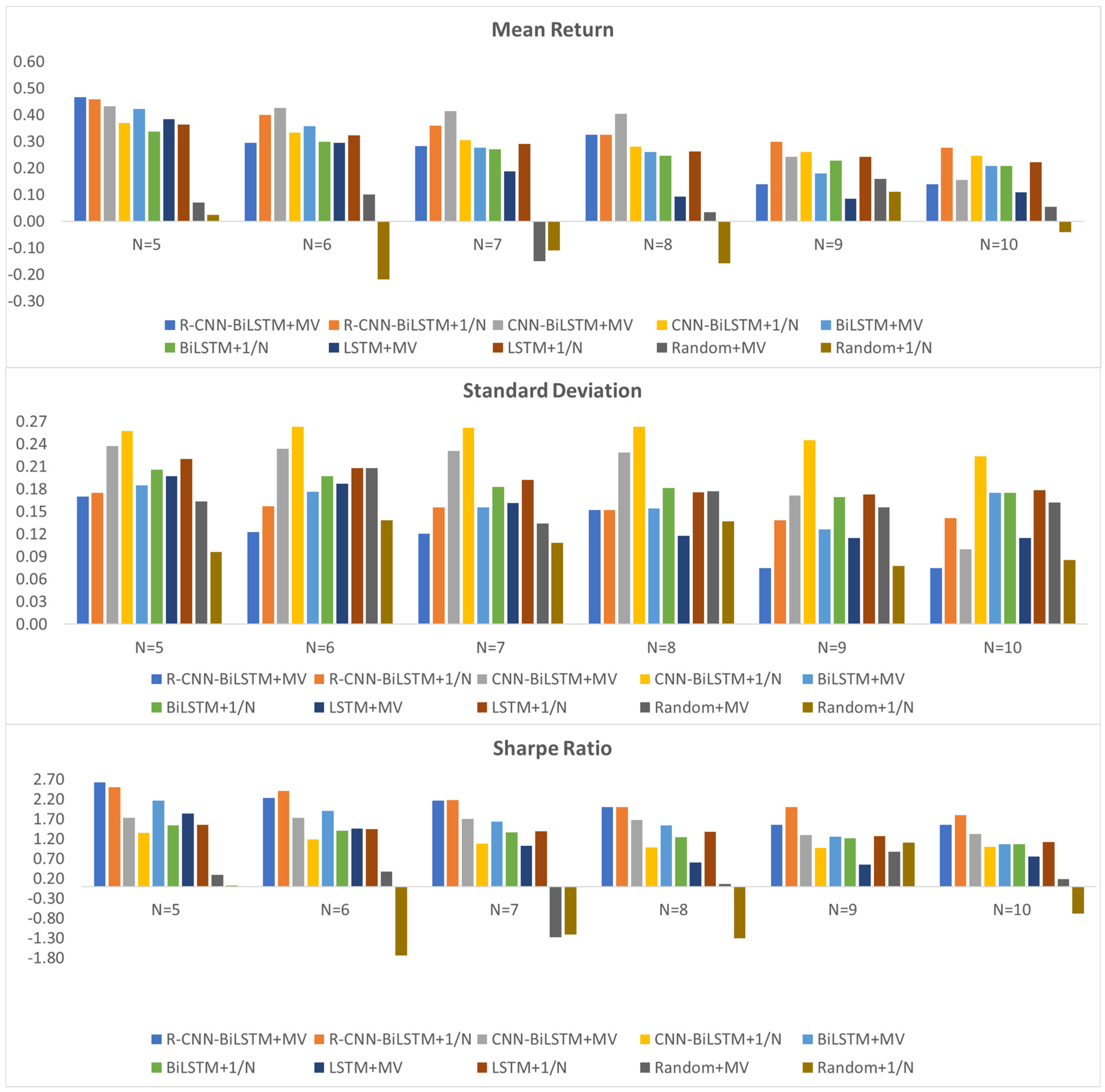
Numerous studies have shown that holding too many different stocks makes them hard to control and manage, especially for individual investors. Several studies related to portfolio optimization consider building a portfolio with fewer than 10 stocks (Almahdi and Yang 2017). Paiva et al. (2019) found that a portfolio with an average of seven stocks outperforms other portfolios with a different number of stocks. Wang et al. (2020) showed that the optimal portfolio with ten stocks performs better than a portfolio with other numbers of stocks. Chen et al. (2021) argued that having seven stocks in a portfolio is the most appropriate number for portfolio formation. As a result, this study decides to construct portfolios corresponding to the number of stocks N = 5, 6, 7, 8, 9, and 10 and to comprehensively evaluate the performance of the proposed models. Annualized mean return, annualized standard deviation, and annualized Sharpe ratio are employed as indicators.
According to Figure 4, the annualized performance for different sizes of portfolios N = 5, 6, 7, 8, 9, and 10 are presented in three sub-graphs in which the Y-axis of each subgraph indicates the amount of mean return, standard deviation, and Sharpe ratio computed annually, while the X-axis of each subgraph represents the different models, which are formed by a different number of stocks. It can be clearly seen from Figure 4 that when the number of N = 5, R-CNN-BiLSTM+MV performs the best in terms of mean return, standard deviation, and Sharp ratio. More precisely, when N = 5, R-CNN-BiLSTM+MV has the highest mean return of 0.47, followed by 0.46 for R-CNN-BiLSTM+1/N, 0.43 for CNN-BiLSTM+MV, 0.42 for BiLSTM+MV, 0.38 for LSTM+MV, 0.37 for CNN+BiLSTM+1/N, 0.36 for LSTM+1/N, 0.34 for BiLSTM+1/N, 0.07 for Random+MV, and 0.02 for Random+1/N. Furthermore, when N = 9 and 10, R-CNN-BiLSTM+MV outperforms the other models in terms of standard deviation. Specifically, R-CNN-BiLSTM+MV has the lowest standard deviation of 0.07 for both N = 9 and 10. As for the Sharpe ratio measurement, when N = 5, 8, R-CNN-BiLSTM+MV provides the best Sharpe ratios of 2.62 and 1.99, respectively. However, R-CNN-BiLSTM+1/N also has the same Sharpe ratio as R-CNN-BiLSTM+MV when N = 8.
In summary, a clear advantage of R-CNN-BiLSTM+MV is found with a portfolio size N = 5 in which all three indicators outperform the other models except for the risk of Random+MV and Random+1/N; however, these two models have low expected returns of 0.07 and 0.02, respectively, but it is still reasonable to consider R-CNN-BiLSTM+MV superior. Furthermore, most of the models tend to perform better in terms of annualized expected return, annualized Sharpe ratio, and annualized standard deviation or risk when the number of stocks in the portfolio is five.
6. Discussion and Conclusions
6.1. Discussion and Key Findings
The paper aims to extend the existing literature on portfolio optimization with stock selection. The proposed prediction model is developed based on the use of robust statistics theory and CNN-BiLSTM machine learning model to advance the MV model, which incorporates the advantages of machine learning into stock selection. This study has several findings.
First, this paper compares the predictive performance of LSTM, BiLSTM, CNN-BiLSTM, and stock prediction. The experimental results show that BiLSTM is superior to the other models, which indicates that it is more suitable for financial time-series prediction than the other machine models applied in this experiment, confirming the study by Wang et al. (2020) showing that that traditional LSTM was superior in terms of prediction performance.
Second, this study improves the predictive accuracy of the CNN-BiLSTM by transforming the stock closing price into a robust input feature that can effectively reduce the error of the prediction before the model predicts the future price. After comparing the outcomes of the R-CNN-BiLSTM to LSTM, BiLSTM, and CNN-BiLSTM, it was discovered that the robust input is appropriate to use as an input feature for the machine learning training process to capture financial time-series data that can overcome the other comparison models when the direct stock closing price is used as the input feature.
Finally, the result from the prediction process is incorporated into stock selection for portfolio optimization; the stocks with higher returns calculated from predicted prices are chosen to construct the optimal portfolio. The experimental results show that holding five stocks is appropriate and realistic for individual investors, which is different from the results Wang et al. (2020) and Chen et al. (2021). Additionally, most of the results of R-CNN-BiLSTM+MV, R-CNN-BiLSTM+1/N, CNN-BiLSTM+MV, CNN-BiLSTM+1/N, BiLSTM+MV, BiLSTM+1/N, LSTM+MV, and LSTM+1/N are superior to both Random+MV and Random+1/N in terms of the Sharpe ratio, mean return, and standard deviation, which indicates the significance of selecting high-quality stocks in portfolio optimization. The significance of stock preselection is similar to the conclusions by Wang et al. (2020), Ta et al. (2020), and Chen et al. (2021).
6.2. Theoretical Implications
This study enriches the theoretical research on stock price prediction and portfolio optimization. This paper uses four prediction models, which can capture the financial time-series data to guarantee high-quality assets before commencing portfolio optimization. Specifically, LSTM, BiLSTM, CNN-BiLSTM, and R-CNN-BiLSTM are adopted to predict the daily future close price of the stock and compare the forecasting outcomes of R-CNN-BiLSTM with LSTM, BiLSTM, and CNN-BiLSTM to show the predictability of R-CNN-BiLSTM using robust input instead of the direct stock closing price in more accurately predicting financial time-series data.
6.3. Limitations and Future Work
Although this study provides useful insights, there are some limitations. First, we only use the stock data in Thailand. Due to different economics between countries, this method might not be suitable for stock markets in other countries. Second, there are several external factors that impact the financial market and can be added as input indicators to improve the method, such as COVID-19 crisis, interest rates, and politics. Third, this study does not consider time complexity as a constraint to compare the results. Finally, since this study sets hyperparameters manually based on trial and error, applying hyperparameter optimization algorithms may provide better hyperparameters.
In future research, time complexity should be considered to further demonstrate the applicability of the proposed method.
Author Contributions
Conceptualization, A.C. and R.C.; Data curation, A.C.; Formal analysis, A.C.; Investigation, A.C.; Methodology, A.C. and R.C.; Supervision, R.C.; Validation, R.C.; Visualization, A.C.; Writing—original draft, A.C.; Writing—review and editing, R.C. All authors have read and agreed to the published version of the manuscript.
Funding
This research received no external funding.
Institutional Review Board Statement
Not applicable.
Informed Consent Statement
Not applicable.
Data Availability Statement
Dataset available at https:www.//finance.yahoo.com, accessed on 30 January 2022.
Conflicts of Interest
The authors declare no conflict of interest.
| 1 | R-CNN-BiLSTM is used for stock prediction before optimizing the portfolio using the 1/N model. |
References
- Abrami, Rizkar, and Santoso Marsoem. 2021. Optimal portfolio Formation with Single Index Model Approach on Lq-45 Stocks on Indonesia Stock Exchange. International Journal of Innovative Science and Research Technology 6: 1301–1309. [Google Scholar]
- Albawi, Saad, Tareq A. Mohammed, and Saad Al-Zawi. 2017. Understanding of a convolutional neural network. Paper presented at 2017 International Conference on Engineering and Technology (ICET), Antalya, Turkey, August 21–23. [Google Scholar]
- Alizadeh, Meysam, Roy Rada, Fariboz Jolai, and Elnaz Fotoohi. 2010. An adaptive neuro-fuzzy system for stock portfolio analysis. International Journal of Intelligent Systems 26: 99–114. [Google Scholar] [CrossRef]
- Almahdi, Saud, and Steve Y. Yang. 2017. An adaptive portfolio trading system: A risk-return portfolio optimization using recurrent reinforcement learning with expected maximum drawdown. Expert Systems with Applications 87: 267–79. [Google Scholar] [CrossRef]
- Beheshti, Bijan. 2018. Effective stock selection and portfolio construction within US, International, and emerging markets. Frontiers in Applied Mathematics and Statistics 4: 17. [Google Scholar] [CrossRef]
- Ben Salah, Hanen, Jan G. De Gooijer, Ali Gannoun, and Mathieu Ribatet. 2018. Mean–variance and mean–semivariance portfolio selection: A multivariate nonparametric approach. Financial Markets and Portfolio Management 32: 419–36. [Google Scholar] [CrossRef]
- Bodnar, Taras, Stepan Mazur, and Yarema Okhrin. 2017. Bayesian estimation of the global minimum variance portfolio. European Journal of Operational Research 256: 292–307. [Google Scholar] [CrossRef] [Green Version]
- Brown, David B., and Jame E. Smith. 2011. Dynamic portfolio optimization with transaction costs: Heuristics and dual bounds. Management Science 57: 1752–70. [Google Scholar] [CrossRef] [Green Version]
- Chen, Wei, Haoyu Zhang, Mukesh Kumar Mehlawat, and Lifen Jia. 2021. Mean–variance portfolio optimization using machine learning-based stock price prediction. Applied Soft Computing 100: 106943. [Google Scholar] [CrossRef]
- Dixon, Matthew F., Igor Halperin, and Paul Bilokon. 2020. Machine Learning in Finance. Berlin and Heidelberg: Springer International Publishing. [Google Scholar]
- Dong, Li, Furu Wei, Chuanqi Tan, Duyu Tang, Ming Zhou, and Ke Xu. 2014. Adaptive Recursive Neural Network for Target-dependent Twitter Sentiment Classification. In Proceedings of the 52nd Annual Meeting of the Association for Computational Linguistics (Volume 2: Short Papers). Baltimore: Association for Computational Linguistics, pp. 49–54. [Google Scholar] [CrossRef] [Green Version]
- Fischer, Thomas, and Christopher Krauss. 2018. Deep learning with long short-term memory networks for financial market predictions. European Journal of Operational Research 270: 654–69. [Google Scholar] [CrossRef] [Green Version]
- Fox, John, and Sanford Weisberg. 2019. An R Companion to Applied Regression. New York: SAGE Publication, Inc. [Google Scholar]
- Gao, Yo, Rong Wang, and Enmin Zhou. 2021. Stock prediction based on optimized LSTM and GRU models. Scientific Programming 2021: 4055281. [Google Scholar] [CrossRef]
- Hampel, Frank, Christian Hennig, and Elvezio Ronchetti. 2011. A smoothing principle for the Huber and other location M-estimators. Computational Statistics & Data Analysis 55: 324–37. [Google Scholar] [CrossRef]
- Hastie, Trevor, Jerome Friedman, and Robert Tisbshirani. 2017. The Elements of Statistical Learning: Data Mining, Inference, and Prediction. Berlin and Heidelberg: Springer. [Google Scholar]
- Henrique, Bruno M., Vinicius A. Sobreiro, and Herbert Kimura. 2019. Literature review: Machine learning techniques applied to financial market prediction. Expert Systems with Applications 124: 226–51. [Google Scholar] [CrossRef]
- Hochreiter, Sepp, and Jurgen Schmidhuber. 1997. Long short-term memory. Neural Computation 9: 1735–80. [Google Scholar] [CrossRef] [PubMed]
- Huang, Chien-Feng. 2012. A hybrid stock selection model using genetic algorithms and support vector regression. Applied Soft Computing 12: 807–18. [Google Scholar] [CrossRef]
- Huang, Ripeng, Shaojian Qu, Xiaoguang Yang, Fengmin Xu, Zeshui Xu, and Wei Zhou. 2021. Sparse portfolio selection with uncertain probability distribution. Applied Intelligence 51: 6665–84. [Google Scholar] [CrossRef]
- Huber, Peter J. 1964. Robust estimation of a location parameter. The Annals of Mathematical Statistics 35: 73–101. [Google Scholar] [CrossRef]
- Jierula, Alipujiang, Shuhong Wang, Tae-Min OH, and Pengyu Wang. 2021. Study on accuracy metrics for evaluating the predictions of damage locations in deep piles using artificial neural networks with acoustic emission data. Applied Sciences 11: 2314. [Google Scholar] [CrossRef]
- Katsikis, Vasilios N., Spyridon D. Mourtas, Predrag S. Stanimirović, Shuai Li, and Xinwei Cao. 2021. Time-varying mean-variance portfolio selection under transaction costs and cardinality constraint problem via beetle antennae search algorithm (BAS). Operations Research Forum 2: 18. [Google Scholar] [CrossRef]
- Khan, Ameer Hamza, Xinwei Cao, Vasilio N. Katsikis, Predrag Stanimirovic, Ivona Brajevic, Shuai Li, Seifedine Kadry, and Y. Nam. 2020. Optimal portfolio management for engineering problems using nonconvex cardinality constraint: A computing perspective. IEEE Access 8: 57437–50. [Google Scholar] [CrossRef]
- Khan, Ameer Tamoor, Xinwei Cao, Inova Brajevic, Predrag S. Stanimirovic, Vasilio N. Katsikis, and Shuai Li. 2022. Non-linear activated beetle antennae search: A novel technique for non-convex tax-aware portfolio optimization problem. Expert Systems with Applications 197: 116631. [Google Scholar] [CrossRef]
- Khan, Ameer Tamoor, Xinwei Cao, Shuai Li, Bin Hu, and Vasilio N. Katsikis. 2021. Quantum beetle antennae search: A novel technique for the constrained portfolio optimization problem. Science China Information Sciences 64: 152204. [Google Scholar] [CrossRef]
- Kolm, Petter N., Reha Tütüncü, and Frank J. Fabozzi. 2014. 60 years of portfolio optimization: Practical challenges and current trends. European Journal of Operational Research 234: 356–71. [Google Scholar] [CrossRef]
- Le Caillec, Jean-Marc, Alya Itani, Didier Guriot, and Yves Rakotondratsimba. 2017. Stock picking by probability–possibility approaches. IEEE Transactions on Fuzzy Systems 25: 333–49. [Google Scholar] [CrossRef]
- Lefebvre, William, Gregoire Loeper, and Huyen Pham. 2020. Mean-variance portfolio selection with Tracking Error Penalization. Mathematics 8: 1915. [Google Scholar] [CrossRef]
- Li, Ting, Weiguo Zhang, and Weijun Xu. 2015. A fuzzy portfolio selection model with background risk. Applied Mathematics and Computation 256: 505–13. [Google Scholar] [CrossRef]
- Lozza, Sergio Ortobelli, Enrico Angelelli, and Daniele Toninelli. 2011. Set-portfolio selection with the use of market stochastic bounds. Emerging Markets Finance and Trade 47: 5–24. [Google Scholar] [CrossRef] [Green Version]
- Ma, Yilin, Ruizhu Han, and Weizhing Wang. 2021. Portfolio optimization with return prediction using Deep Learning and machine learning. Expert Systems with Applications 165: 113973. [Google Scholar] [CrossRef]
- Markowitz, Harry. 1952. Portfolio selection*. The Journal of Finance 7: 77–91. [Google Scholar] [CrossRef]
- Maronna, Ricardo A., Douglas Martin, and Víctor J. Yohai. 2006. Robust Statistics: Theory and Methods. Hoboken: John Wiley & Sons. [Google Scholar]
- Maronna, Ricardo A., Douglas Martin, Victor J. Yohai, and Matías Salibián-Barrera. 2019. Robust Statistics Theory and Methods (with R). Hoboken: John Wiley & Sons. [Google Scholar]
- Mba, Jules Clement, Kofi Agyarko Ababio, and Samuel Kwaku Agyei. 2022. Markowitz mean-variance portfolio selection and optimization under a behavioral spectacle: New empirical evidence. International Journal of Financial Studies 10: 28. [Google Scholar] [CrossRef]
- Milošević, Nemanja, and Milos Racković. 2019. Classification based on missing features in deep convolutional neural networks. Neural Network World 29: 221–34. [Google Scholar] [CrossRef]
- Mitra Thakur, Gour Sundar, Rupak Bhattacharyya, and Seema Sarkar (Mondal). 2018. Stock portfolio selection using Dempster–Shafer Evidence theory. Journal of King Saud University-Computer and Information Sciences 30: 223–35. [Google Scholar] [CrossRef] [Green Version]
- Nguyen, Than Thi. 2014. Selection of the right risk measures for portfolio allocation. International Journal of Monetary Economics and Finance 7: 135. [Google Scholar] [CrossRef]
- Ortiz, Roberto, Mauricio Contreras, and Cristhian Mellado. 2021. Improving the volatility of the optimal weights of the Markowitz model. Economic Research-Ekonomska Istraživanja, September 29. [Google Scholar] [CrossRef]
- Paiva, Felipe D., Rodrigo T. Cardoso, Gustova P. Hanaoka, and Wendel M. Duarte. 2019. Decision-making for financial trading: A fusion approach of machine learning and portfolio selection. Expert Systems with Applications 115: 635–55. [Google Scholar] [CrossRef]
- Rahiminezhad Galankashi, Masoud, Farimah Mokhatab Rafiei, and Maryam Ghezelbash. 2020. Portfolio selection: A fuzzy-ANP approach. Financial Innovation 6: 17. [Google Scholar] [CrossRef]
- Rather, Akhter M., Arun Agarwal, and V. N. Sastry. 2015. Recurrent neural network and a hybrid model for prediction of Stock returns. Expert Systems with Applications 42: 3234–41. [Google Scholar] [CrossRef]
- Sadouk, Lamyaa. 2019. CNN approaches for Time Series Classification. Time Series Analysis-Data, Methods, and Applications, November 5. [Google Scholar] [CrossRef] [Green Version]
- Sharpe, William F., and Harry M. Markowitz. 1989. Mean-variance analysis in portfolio choice and capital markets. The Journal of Finance 44: 531. [Google Scholar] [CrossRef]
- Siami-Namini, Sima, Neda Tavakoli, and Akbar S. Namin. 2019. The performance of LSTM and BiLSTM in forecasting time series. Paper presented at 2019 IEEE International Conference on Big Data (Big Data), Los Angeles, CA, USA, December 9–12. [Google Scholar]
- Sikalo, Mirza, Almira Arnaut-Berilo, and Azra Zaimovic. 2022. Efficient Asset Allocation: Application of game theory-based model for superior performance. International Journal of Financial Studies 10: 20. [Google Scholar] [CrossRef]
- Singh, Upma, Mohammad Rizwan, Muhannad Alaraj, and I. Alsaidan. 2021. A machine learning-based gradient boosting regression approach for wind power production forecasting: A step towards Smart Grid Environments. Energies 14: 5196. [Google Scholar] [CrossRef]
- Soeryana, E., N. Fadhlina, Sukono, E. Rusyaman, and S. Supian. 2017. Mean-variance portfolio optimization by using time series approaches based on logarithmic utility function. IOP Conference Series: Materials Science and Engineering 166: 012003. [Google Scholar] [CrossRef] [Green Version]
- Ta, Van-Dai, Chuan-Ming Liu, and Direselign A. Tadesse. 2020. Portfolio optimization-based stock prediction using long-short term memory network in quantitative trading. Applied Sciences 10: 437. [Google Scholar] [CrossRef] [Green Version]
- Tu, Juntu, and Guofu Zhou. 2010. Incorporating economic objectives into bayesian priors: Portfolio choice under parameter uncertainty. Journal of Financial and Quantitative Analysis 45: 959–86. [Google Scholar] [CrossRef]
- Wan, Yuqing, Raymond Y. Lau, and Yain-Whar Si. 2020. Mining subsequent trend patterns from financial time series. International Journal of Wavelets, Multiresolution and Information Processing 18: 2050010. [Google Scholar] [CrossRef]
- Wang, Wuyu, Weizi Li, Ning Zhang, and Kecheng Liu. 2020. Portfolio formation with preselection using deep learning from long-term financial data. Expert Systems with Applications 143: 113042. [Google Scholar] [CrossRef]
- Yang, Mo, and Jing Wang. 2022. Adaptability of Financial Time Series prediction based on bilstm. Procedia Computer Science 199: 18–25. [Google Scholar] [CrossRef]
- Zaimovic, Azra, Adna Omanovic, and Almira Arnaut-Berilo. 2021. How many stocks are sufficient for equity portfolio diversification? A review of the literature. Journal of Risk and Financial Management 14: 551. [Google Scholar] [CrossRef]
Figure 1.
The scheme of the proposed model.

Figure 2.
The framework of CNN model.

Figure 3.
The framework of BiLSTM model.

Figure 4.
Annualizedportfolio performance for different sizes of portfolios.


Table 1.
Summary statistics for experimental data (Thai baht).
| Stock | Maximum | Minimum | Mean | Standard Deviation |
|---|---|---|---|---|
| AOT | 81 | 25.4 | 52.74 | 15.72 |
| BDMS | 27.25 | 17.5 | 22.26 | 2.27 |
| BEM | 12 | 4.07 | 7.8 | 2.06 |
| BJC | 66 | 27.22 | 44.42 | 9.12 |
| BTS | 14.2 | 7.85 | 9.79 | 1.53 |
| CPALL | 90 | 37.5 | 63.81 | 13.46 |
| CPN | 86.25 | 33.25 | 60.99 | 13.53 |
| DELTA | 684 | 30 | 81.12 | 44.62 |
| DTAC | 96.25 | 27.75 | 48.93 | 15.18 |
| EA | 69.5 | 19.1 | 36.46 | 11.48 |
| GLOBAL | 19.61 | 6.33 | 13.24 | 3.58 |
| INTUCH | 83.5 | 43 | 59.31 | 8.8 |
| IRPC | 8.15 | 1.88 | 4.77 | 1.38 |
| IVL | 62.5 | 16.9 | 36.27 | 12.24 |
| KCE | 64.5 | 12 | 34.45 | 12.31 |
| KTC | 60 | 6.22 | 23.28 | 13.15 |
| LH | 12.2 | 6 | 9.53 | 1.26 |
| MINT | 45.25 | 13.49 | 34.28 | 6.63 |
| MTC | 68.25 | 12 | 36.75 | 15.01 |
| PTT | 58.8 | 19.8 | 39.54 | 8.32 |
| PTTEP | 160 | 42.5 | 101.83 | 23.64 |
| PTTGC | 103 | 24 | 63.98 | 14.4 |
| RATCH | 81.5 | 46 | 56.01 | 6.73 |
| SAWAD | 78.75 | 19.49 | 43.52 | 11.55 |
| SCC | 550 | 267 | 454.1 | 59.68 |
Table 2.
Comparison of prediction performance between LSTM and BiLSTM.
| Stock | LSTM | BiLSTM | ||||
|---|---|---|---|---|---|---|
| MAE | MSE | SMAPE | MAE | MSE | SMAPE | |
| AOT | 1.8492 | 6.0365 | 1.4947 | 1.3972 | 3.8694 | 1.1617 |
| BDMS | 0.3848 | 0.2955 | 0.9173 | 0.3652 | 0.2743 | 0.8640 |
| BEM | 0.2085 | 0.0845 | 1.1439 | 0.2095 | 0.0897 | 1.1524 |
| BJC | 0.9812 | 1.7666 | 1.2952 | 1.1242 | 2.1052 | 1.4813 |
| BTS | 0.2837 | 0.1599 | 1.2865 | 0.2313 | 0.1095 | 1.0495 |
| CPALL | 0.9605 | 1.6107 | 0.7317 | 0.9228 | 1.5193 | 0.7042 |
| CPN | 1.8462 | 7.1009 | 1.9229 | 1.7676 | 6.5828 | 1.8486 |
| DELTA | 4.0368 | 8.0218 | 13.123 | 3.8862 | 7.7699 | 12.226 |
| DTAC | 0.9254 | 1.5075 | 1.1961 | 0.9695 | 1.5263 | 1.2567 |
| EA | 1.0341 | 2.0658 | 1.2442 | 1.0010 | 1.9209 | 1.2035 |
| GLOBAL | 0.4385 | 0.3665 | 1.5382 | 0.4237 | 0.3466 | 1.4796 |
| IRPC | 0.7735 | 0.6996 | 1.3212 | 0.6152 | 0.4566 | 1.0894 |
| INTUCH | 0.7602 | 1.3049 | 0.7142 | 0.7457 | 1.2532 | 0.7002 |
| IVL | 1.1677 | 2.4750 | 2.2526 | 1.1137 | 2.1696 | 2.1337 |
| KCE | 1.3583 | 2.9136 | 3.0482 | 1.2504 | 2.6176 | 2.9376 |
| KTC | 1.6230 | 7.4166 | 2.0531 | 1.5991 | 7.5624 | 2.0145 |
| LH | 0.4567 | 0.3537 | 3.0500 | 0.3830 | 0.2645 | 2.5767 |
| MINT | 4.2719 | 2.5754 | 9.3568 | 3.5595 | 1.8810 | 7.9947 |
| MTC | 2.9454 | 1.3472 | 2.7505 | 2.2480 | 8.7324 | 2.1013 |
| PTT | 0.9246 | 2.2412 | 1.2935 | 0.9153 | 2.0173 | 1.2794 |
| PTTEP | 2.6926 | 2.1457 | 1.5534 | 2.5247 | 2.0952 | 1.4822 |
| PTTGC | 4.7754 | 4.1757 | 5.5750 | 3.2552 | 2.5053 | 3.9878 |
| RATCH | 1.0472 | 2.4033 | 0.8817 | 1.3077 | 3.1643 | 1.0816 |
| SAWAD | 3.8613 | 3.1299 | 3.2622 | 3.5476 | 2.5694 | 2.9785 |
| SCC | 3.6151 | 1.7271 | 4.9859 | 2.6922 | 1.0819 | 3.7868 |
Table 3.
Comparison of prediction performance between CNN-BiLSTM and R-CNN-BiLSTM.
| Stock | CNN-BiLSTM | R-CNN-BiLSTM | ||||
|---|---|---|---|---|---|---|
| MAE | MSE | SMAPE | MAE | MSE | SMAPE | |
| AOT | 1.3178 | 3.3801 | 1.0902 | 1.3700 | 3.1541 | 1.1104 |
| BDMS | 0.4277 | 0.3319 | 1.0172 | 0.3292 | 0.1934 | 0.7758 |
| BEM | 0.1651 | 0.0585 | 0.9034 | 0.1747 | 0.0523 | 0.9577 |
| BJC | 1.0290 | 1.8592 | 1.3327 | 0.8566 | 1.1691 | 1.1343 |
| BTS | 0.3006 | 0.2078 | 1.3639 | 0.2627 | 0.1243 | 1.1716 |
| CPALL | 1.0490 | 2.0394 | 0.7842 | 0.7528 | 1.0157 | 0.5713 |
| CPN | 1.8837 | 6.6585 | 1.9341 | 1.2533 | 2.8825 | 1.3019 |
| DELTA | 4.1104 | 8.1768 | 13.487 | 3.4162 | 5.0508 | 12.143 |
| DTAC | 1.1074 | 1.9661 | 1.4468 | 0.8781 | 1.2819 | 1.1335 |
| EA | 0.9578 | 1.6883 | 1.1501 | 0.8770 | 1.3480 | 1.0603 |
| GLOBAL | 0.3636 | 0.2451 | 1.2451 | 0.3325 | 0.2011 | 1.1091 |
| IRPC | 0.7817 | 1.2752 | 0.7347 | 0.7434 | 1.1314 | 0.6960 |
| INTUCH | 0.7479 | 0.7327 | 1.2883 | 0.9645 | 1.0976 | 1.5837 |
| IVL | 0.9090 | 1.5083 | 1.7234 | 0.8079 | 1.0826 | 1.5329 |
| KCE | 1.2586 | 2.5306 | 2.8828 | 0.7679 | 0.9975 | 1.7225 |
| KTC | 1.8072 | 8.4518 | 2.3359 | 0.9608 | 2.2998 | 1.2831 |
| LH | 0.4215 | 0.3194 | 2.8259 | 0.4915 | 0.3743 | 3.2514 |
| MINT | 3.1798 | 1.5235 | 7.2280 | 3.1251 | 1.3556 | 7.0846 |
| MTC | 2.2111 | 9.3412 | 2.0425 | 1.8174 | 6.4816 | 1.6748 |
| PTT | 0.7665 | 1.2902 | 1.0616 | 0.6891 | 0.9916 | 0.9468 |
| PTTEP | 2.0733 | 1.1074 | 1.1690 | 2.0274 | 1.0305 | 1.1313 |
| PTTGC | 4.7207 | 4.3939 | 5.5390 | 5.1528 | 4.9323 | 5.9606 |
| RATCH | 1.1446 | 2.8712 | 0.9626 | 1.0720 | 2.0291 | 0.8916 |
| SAWAD | 3.5888 | 2.8325 | 2.9873 | 3.6310 | 3.0988 | 3.0133 |
| SCC | 2.0515 | 7.7104 | 2.9372 | 3.7010 | 1.8256 | 5.0882 |
Publisher’s Note: MDPI stays neutral with regard to jurisdictional claims in published maps and institutional affiliations. |
© 2022 by the authors. Licensee MDPI, Basel, Switzerland. This article is an open access article distributed under the terms and conditions of the Creative Commons Attribution (CC BY) license (https://creativecommons.org/licenses/by/4.0/).
Share and Cite
MDPI and ACS Style
Chaweewanchon, A.; Chaysiri, R. Markowitz Mean-Variance Portfolio Optimization with Predictive Stock Selection Using Machine Learning. Int. J. Financial Stud. 2022, 10, 64. https://0-doi-org.brum.beds.ac.uk/10.3390/ijfs10030064
AMA Style
Chaweewanchon A, Chaysiri R. Markowitz Mean-Variance Portfolio Optimization with Predictive Stock Selection Using Machine Learning. International Journal of Financial Studies. 2022; 10(3):64. https://0-doi-org.brum.beds.ac.uk/10.3390/ijfs10030064
Chicago/Turabian StyleChaweewanchon, Apichat, and Rujira Chaysiri. 2022. "Markowitz Mean-Variance Portfolio Optimization with Predictive Stock Selection Using Machine Learning" International Journal of Financial Studies 10, no. 3: 64. https://0-doi-org.brum.beds.ac.uk/10.3390/ijfs10030064
Note that from the first issue of 2016, this journal uses article numbers instead of page numbers. See further details here.