Tick Size and Price Reversal after Order Imbalance

Abstract

It is well known that intraday returns tend to reverse the following intraday period, conditional on excess buying pressure on the bid or ask side. This suggests that liquidity providers “overreact” to order imbalance (OIB) by initially altering quotes so much that a negative autocorrelation is seen in mid-price returns. We investigate under which circumstances this behavior is most common. Specifically, it seems the tick size augments “OIB-reversal”. However, if the tick size is binding for much of the trading day, it has the opposite effect of censoring such reversals. In addition, if market liquidity is high, the reversal becomes more frequent.

1. Introduction

Chordia et al. (2005) found that NYSE specialists tend to adjust their quotes in the opposite direction of arriving trades. This causes a significant negative autocorrelation in returns, conditional on the difference between buyer and seller-initiated trades. This difference is called order imbalance (OIB), and we refer to the tendency that prices tend to reverse conditional on this as the OIB-reversal effect.

The main contribution of this paper is an improved understanding of how the tick size interacts with liquidity provision and OIB. Specifically, our results suggest that the tick size in general augments changes in quotes on average. This, in turn, leads to a negative autocorrelation conditioned on order imbalance (OIB-reversal).

The perhaps most surprising discovery in the original paper by Chordia et al. was that liquidity providers act seemingly irrational by altering their quotes “too much” when faced with increasing order imbalance. When, for example, many buyers arrived at the marketplace, the specialists at NYSE systematically retracted their ask orders so much that it resulted in a predictable mid-price reversal the next period. Since the quotes predictably would have to be reentered next period, it seems the specialists systematically made mistakes they had to mend later. Chordia et. al. suggested that this behavior has to do with balancing the specialists’ inventory, but they did not investigate further which market conditions were associated with this reversal. In this paper, we therefore take a closer look at under which circumstances OIB-reversal occurs.

We confirm the OIB-reversal effect based on data from the Norwegian stock market. The OIB-reversal is defined as the difference between the unconditional autocorrelation and the autocorrelation conditional on OIB. In contrast to Chordia et al. (2005), we find a significant unconditional autocorrelation in mid-price returns, though the unconditional autocorrelation is significantly smaller than the conditional. This is perhaps too small to overcome the spread and being exploited economically. We therefore make the conjecture that these findings are consistent with Chordia et al. (2005).

We then investigate under which market conditions the OIB-reversal effect is most prevalent. The market conditions we consider are the spread, the tick size, the frequency at which the tick size is binding, the order book size, the share of total market cap, the number of trades, and the volatility.

The tick size, the smallest permissible quote difference, can be considered reasonably exogenous in the short run relevant for this study. If the tick size is sufficiently big, it may be an obstacle for OIB-reversal. Altering quotes too much may attract arbitrageurs on the limit side who exploit large and predictable reversals after buying or selling pressure. If the tick size makes a suitable change in quotes impossible, the liquidity provider may maintain current quotes and perhaps instead reduce volumes posted. This would reduce the frequency of reversals, censoring the number of times reversals occur and reducing liquidity. We call this the censoring effect.

However, an increase in tick size may also exaggerate the size of the reversal if it forces the liquidity provider to raise the initial price more than with a smaller tick size. We would expect this to happen more often if the constraints imposed by the tick size are not “too severe”. We call this the augmentation effect.

Depending on whether censoring or augmentation is the most prevalent, we would expect the coefficient of tick size in a regression on OIB-reversal to be negative or positive, respectively. However, both these effects are probably present in the data. We therefore also investigate what may cause the effect to switch between censoring and augmentation.

We can measure the severity of the constraints imposed by the tick size by observing the frequency at which the tick size is binding (bind frequency). A tick size that is more frequently binding is more restrictive. Since censoring probably occurs more often when the tick size is a bigger obstacle, we would expect augmentation to become less frequent at the expense of censoring when the tick size often binds. Hence, bind frequency estimated as conditional and unconditional on OIB reversal can provide information to us about how trading in the sample switches from a censoring to an augmentation regime and vice versa.

We also consider the effect of the size of the spread. The spread is similar to bind frequency in that it measures both general liquidity as well as how severely the tick size is a constraint. If tick size is a considerable restriction on price setting, we expect a higher spread in general. However, we expect the bind frequency to be a better measure of constraint severity and the spread to be a relatively better measure of liquidity.

In addition, we also investigate the role of more direct measures of liquidity, namely share of market capitalization, number of trades, and size of order book. We would expect that all of these are positively related to OIB-reversal, since more liquidity is empirically unambiguously associated with a smaller spread, and we expect more frequent reversal when the spread is small. We also investigate the role of volatility on OIB-reversal.

However, if the tick size is too restrictive in the sense that the bind frequency is high, our interpretation of the results is that the probability that quote alteration is censored increases, which leads to less OIB-reversal.

The plan of the paper is as follows. We start with a literature review. In Section 2, we introduce the dataset, and descriptive statistics are presented in Section 3. In Section 4, models and methodology are presented. Results are presented in Section 5, and finally, a short summary is given in Section 6.

2. Literature Review

Chordia et al. (2002) finds that daily returns are positively associated with daily order imbalance, confirming that buying pressure does raise prices. Furthermore, they demonstrate that market returns are still affected by order imbalance, even after controlling for aggregate volume and liquidity. That OIBs are important for daily returns is also confirmed in Chordia and Subrahmanyam (2004). The authors use an intertemporal model in which prices react to autocorrelated imbalances. It turns out that current price movements have a negative relation with lagged imbalances after controlling for the current imbalance. They also investigate the profitability of an imbalance-based trading strategy.

In Chordia et al. (2005), the OIB analysis is extended to intraday data, and the intraday OIB-reversal effect is identified. As mentioned in the introduction, the objective of this paper is to investigate whether the OIB-reversal effect is indeed caused by protective measures against private information.

Chordia et al. (2008) investigate further how known market features are associated with the effect of OIB. Specifically, they analyze the effect of liquidity measured by spread. They find that illiquidity does increase the effect of OIB on returns.

Order imbalance and market efficiency are also studied by Y.-T. Lee et al. (2004). They use data from the Taiwan Stock Exchange. As with the Oslo Stock Exchange, it is also an order driven market with no designated market maker. Lee et al. investigate marketable order imbalances and compute order imbalances based on types of trader, such as individuals, domestic institutions, foreign institutions, and order size of each trader. All trader groups are successful market makers, but large domestic institutions control most of the informed trades, and individual groups are noise or liquidity providers.

In addition, research by Li et al. (2005) examines the effect of order imbalance on the quotation behavior of market markers using a dataset from Nasdaq. Their results show that market markers use both price and quantity quotes when they deal with order imbalances. They also find that order imbalance affects the price movement but not spreads. Additionally, they show that, when public sells (buys) exceed public buys (sells), market makers quote higher quantity of shares. They suggest that market makers intervene to the market by increasing liquidity supply when order imbalance exists in the market.

There has, however, been surprisingly little recent research on order imbalance. It therefore seems to be a possible void in the literature that could be filled by replicating the studies of Chordia et al. on newer data. This could possibly reveal whether computerization has had an impact on the dynamics of order imbalance.

Jegadeesh and Titman (1995) use daily data and find that most of the short horizon return reversals can be explained by the way dealers set bid and ask prices, considering their inventory imbalances. Their study suggests that the decay of the dealer–inventory imbalances takes several days. The trading profits from contrarian trading strategies are found to be compensation for bearing inventory risk.

It is, however, not clear that the OIB-reversal is the result of liquidity providers. In the conventional setup, the market is often modeled similarly to Kyle (1985), where privately informed traders submit market orders and market makers offers quotes. Due to the asymmetric information, market makers must take measures to avoid losses.

However, Kaniel and Liu (2006) find that the informed traders tendency to use limit order may be so high that, in equilibrium, limit orders convey more information than market orders. They also find that the probability of using limit orders is positively related to the time horizon of the private information. This suggests that the mechanism may be very different from the classical setup.

Brown et al. (1997) study the interaction between order imbalance and stock price on the Australian market. They find bi-direct causality between them within a single day. They also suggest that the current return can be explained by the number of orders, while both the current and the future returns can be explained by the dollar value of orders.

In NYSE and Nasdaq, Chan and Fong (2000) find that trade size affects the volatility–volume relation for both markets, and the relation becomes weaker after they control for the return impact of OIB.

Hopman (2007) uses data from the Paris Bourse—also an order driven market. He investigates the explanation of the imbalance between buy and sell orders to stock prices and finds that order flow or imbalance explain most of the changes in stock prices.

Ahn et al. (2002) examine the components of the spread at the Tokyo Stock Market. They find that both adverse selection and order handling cost components show a U-shaped pattern independently.

De Jong et al. (1996) estimate the price effects of trading at the Paris Bourse. Their main results suggest that there is no reversal of the direction of trade. It means that inventory control is unlikely to be important.

Foucault (1999) provides a game theoretic model of price information and decisions in order placement. The article shows that investors can post either limit orders or market orders. While limit orders give time priority, it carries the risk of non-execution.

Comerton-Forde et al. (2010) examine the role of inventories held by market makers and trading revenues. They find that spreads widen when market makers have large inventory positions or poor trading results. They also show that the liquidity of high volatility stocks is more sensitive to inventories and losses than low volatility stocks. Jylhä et al. (2014) investigate where hedge funds are supply or demand liquidity. They show that hedge funds normally supply liquidity but demand liquidity during crisis periods.

Louhichi (2012) shows that there is a causal and dynamic relationship between trading activity and returns relation using intraday data. Trading activity is proxied by the non-directional volume and the directional volume. The directional volume depends on whether the trades are buyer or seller initiated, which is similar to the OIB-measure. The sign of the trades in Louhichi is different from Chordia et al. (2002), which uses an algorithm of C. Lee and Ready (1991). Louhichi determines the trade sign by comparing the time that each order is submitted. He chose this method because he argues that the algorithm of Lee and Ready misclassifies 15% of the transactions. His research highlights a strong bi-directional relationship between directional volume and returns.

3. Data

The data were constructed from the Oslo Stock Exchange (OSE) data feed in the period 2003 to 2009 and contain all orders and trades for all instruments available in that period. Since the sample ends in 2009, it does not cover much of the rise in computerized trading that we have seen in recent years. However, that also makes our sample more similar to the sample of Chordia et al. (2005) in this respect, and we do find that we are able to reproduce their results on OIB, which is essential for the scope of this paper. Of course, this leaves it open for future research to see if computerization has had an impact on OIB and how it interacts with tick size.

OSE is an electronic, fully automated, order driven exchange. The exchange generally does not rely on designated market makers except for some low liquidity stocks. They offer listing and trading in equities, equity certificates, ETFs, fixed income products and derivatives.

The total sample consists of 150 different companies, but for three companies, the liquidity is too poor to estimate any OIB-reversal. The intraday OIB estimation procedure is explained in the next section.

The OIB-reversals are estimated annually for 147 companies across seven years. That results in a highly unbalanced panel, since not all companies are listed at the same time, and OIB-reversals are not possible to estimate for all years. A fully balanced panel would contain 1029 observations, but for the reasons mentioned, the actual number is 637. Additionally, because of interrupted trading, delisting, and relisting and because liquidity is occasionally poor for some companies, the average number of trading days is considerably less than the approximate 225 opening days. After requiring at least 50 trades a day for inclusion in the sample, the actual median and mean numbers of annual trading days in the sample are 145 and 139, respectively. This truncation implies that our results are not valid for low liquidity stocks. This filtering reduces noise and increases the model fit.

There is substantial dispersion in the companies listed on the Oslo Stock Exchange with respect to both size and liquidity. The largest company is Statoil, which is a large corporation even by international standards, ranking as the 67th largest in the world.1 The company has a daily average of 15,000 orders and close to 3000 trades per day, not including transactions on the NYSE, on which it is also listed. On the opposite side of the scale, there are companies with very poor liquidity, thus a minimum amount of trading activity (50 trades per day) is required to be included in the sample.

The most liquid stock in terms of trades per day is Renewable Energy Corporation with 3353 trades per day. The least liquid stock in the sample is Inmeta, with average trades per day equal to the minimum requirement. Hence, the sample contains a mix of liquid and quite illiquid shares.

There is also considerable variation across time, with a substantial increase in trading activity at the end of the sample period. From a research perspective, the dispersion in the dataset is, in many respects, an advantage, since large variations should make it easier to identify effects.

3.1. Reconstructing the Order Book

The database contains the data feed that the OSE sends in real time to its clients. The feed provides information on all the changes to the order book during opening hours. To transform the data into an order book, all the order book changes during a day for a specific company are retrieved from the database. The changes are then processed by an algorithm that reconstructs the order book by sequentially adding, removing, or modifying bids and asks according to the data feed.

After reconstruction, snapshots are taken of all levels in the order book with 60 s intervals. If no orders arrive within a 60 s interval, the snapshot is a copy of the previous order book.

3.2. Order Imbalance and Matching of Trades and Order Book

The order imbalance is, as usual, the number of buyer-initiated trades minus the number of seller-initiated trades. Identification of buyer- and seller-initiated trades requires us to match transactions with changes in limit orders. If, for example, ask orders in the order book change with the same exact quantity at the same price and the same time as a transaction, it is almost certainly a buyer-initiated trade. Louhichi (2012) provides an overview of matching strategies used in the literature.

The matching of our data is summarized in

Table 1. Matching of trades and order book change.

Priority	Matching Requirement	Fraction of All Trades
1	Perfect match, trade and order book change match on price, time (second), and volume	81%
2	Price and time (second) match	5%
3	Price and approximate time (last 5 s) match	2%
4	Time (seconds) match, bid/ask inferred from closest price	3%
5	Approximate match on time (last 5 s), bid/ask inferred from closest price	6%
	Sum	98%

. The matching is done in a prioritized way. First, a perfect match between the order book and the trades is attempted. A perfect match is when the change in the order book and the trade are identical with respect to time, price, and volume.

For those trades that do not meet these criteria, only a match of price and time is required. Then, the same price at the approximate same time (five seconds window) is accepted. If the trade still is not matched, exact match on time is required. However, the trade is assigned to the bid or the ask side by proximity to the transaction price. At last, trades are matched with the change in the order book closest in time (five seconds window) and bid or ask is decided by the proximity to the transaction price. In total, 81% of the trades satisfy the perfect match requirements. Only 2% of the trades are not matched at all.

3.3. Variables

The objective of this paper is to determine how market attributes affect reversal of quotes given order imbalance. This variable is called OIBReversal and is the difference between the intraday unconditional autoregressive coefficient and the autoregressive coefficient conditional on lagged order imbalance. It is explained in more detail how this variable is calculated. In addition, the following independent variables are used:

• LNBindFreq: the log of the frequency at which the tick size is binding
• LNRange: the log of the range volatility measure (the relative difference between opening and closing price)
• LNTrades: the log of the number of trades completed
• LNMarketShare: the log of the share of market capitalization
• LNTotOB: the log of the total amount of orders in the order book
• LNRelTickSize: the log of the average tick size to price ratio
• LNMeanRelSpread: the log of the average relative spread

4. Descriptive Statistics

In the data summary in

Table 2. Data summary.

	Mean	sd	Median	Min	Max	Range	Skew	Kurtosis
OIBReversal	0.037	0.012	0.037	−0.004	0.116	0.12	0.293	1.951
BindFreq	0.614	0.259	0.669	0.001	0.992	0.991	−0.519	−0.801
Range	0.013	0.01	0.01	0.003	0.189	0.186	7.166	90.981
nTrades	937.698	1057.429	530.258	200.647	8399.65	8199.003	2.922	10.983
MarketShare	0.028	0.061	0.007	0	0.477	0.477	3.927	16.919
TotOB (NOK)	14,698,354	24,310,765	7,524,919	355,429	374,826,537	374,471,108	6.328	60.619
RelTickSize	0.003	0.006	0.002	0	0.14	0.14	12.113	212.045
MeanRelSpread	0.005	0.007	0.004	0.001	0.141	0.14	9.808	147.203
LNBindFreq	−0.64	0.67	−0.4	−6.76	−0.01	6.75	−2.23	8.11
LNRange	−4.54	0.52	−4.59	−5.94	−1.67	4.27	0.68	1.41
LNnTrades	6.44	0.83	6.27	5.3	9.04	3.73	0.7	−0.3
LNMarketShare	−4.98	1.88	−4.98	−25.33	−0.74	24.59	−2.04	21.27
LNTotOB (NOK2)	15.93	1	15.83	12.78	19.74	6.96	0.43	0.25
LNRelTickSize	−6.05	0.77	−6.06	−8.57	−1.97	6.61	0.35	2.46
LNMeanRelSpread	−5.57	0.67	−5.59	−7.37	−1.96	5.41	0.71	1.95

OIB: order imbalance.

, we can see that the sample contains almost the entire potential range of the bind frequency [0,1] and that there is a large variation in liquidity measured by the number of trades.

Correlations for the regression variables are reported in

Table 3. Correlation matrix for the regression variables with intraday coefficients calculated with one minute intervals (percent).

	OIBReversal	LNBindFreq	LNRange	LNnTrades	LNMarketShare	LNTotOB	LNRelTickSize
LNBindFreq	9 **
LNRange	13 **	−34 ***
LNnTrades	13 **	2	7 **
LNMarketShare	0	24 ***	−55 ***	42 ***
LNTotOB	13 **	43 ***	−47 ***	63 ***	58 ***
LNRelTickSize	11 **	48 ***	32 ***	−51 ***	−41 ***	−23 ***
LNMeanRelSpread	4 *	−7 **	60 ***	−63 ***	−65 ***	−59 ***	82 ***

Significance codes: * = 0.05, ** = 0.01, *** = 0.001.

, and descriptive statistics on the variables presented in the previous section are summarized in Table 2.

Note, in particular, the correlation between the spread (LNMeanRelSpread) and the liquidity measures LNnTrades, LNMarketShare, and LNTotOB. The spread is, as expected, negatively associated with liquidity.

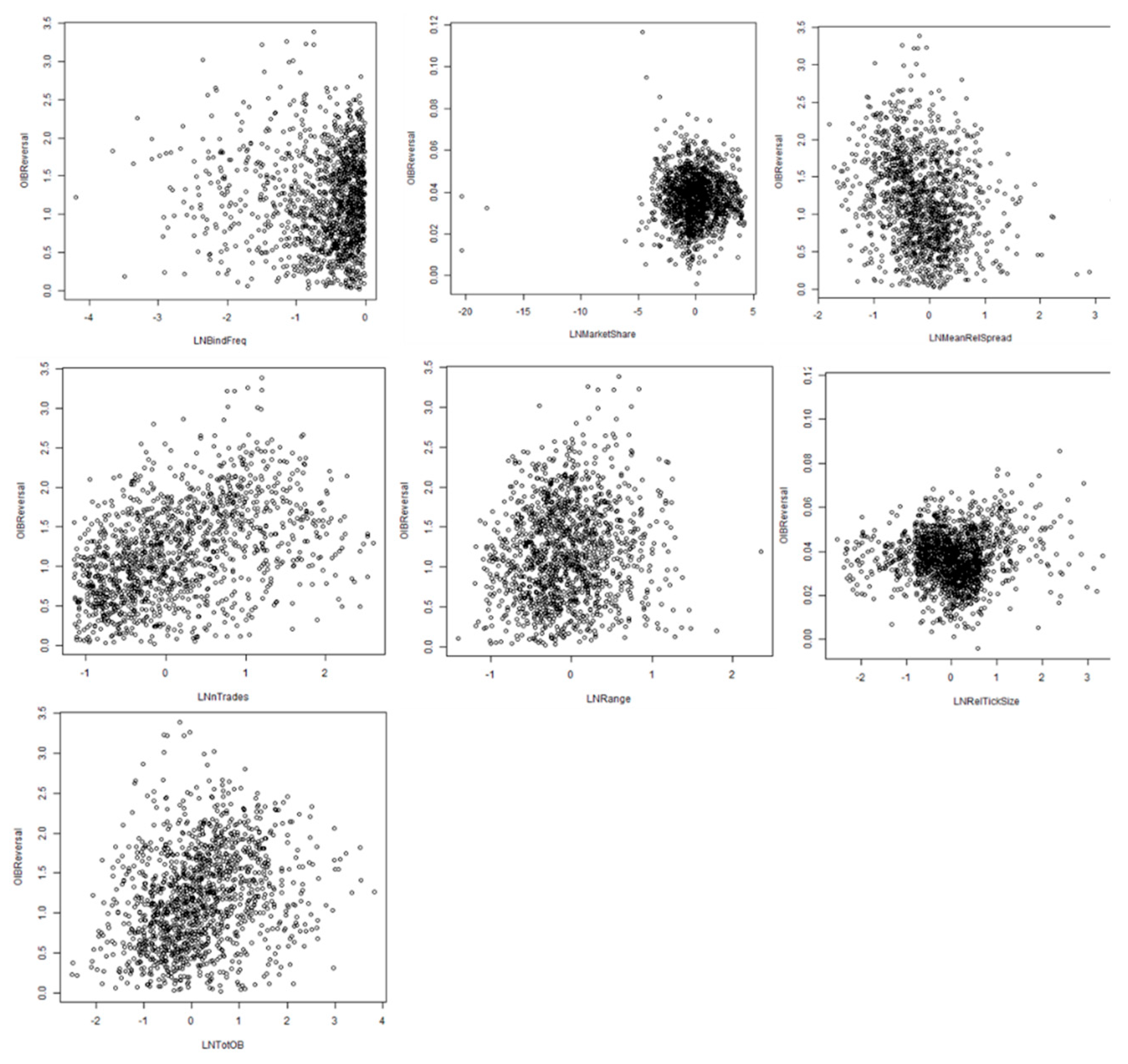
Log–log scatter-plots of the variables are depicted in Figure 1. Most of the variables have a reasonable distribution, and the pattern is consistent with the correlation matrix in Table 3. However, the BindFreq variable seems to be truncated to the right, requiring a dummy for zero values of the log-transformed variable (100% binding tick size). However, it turns out that maximum frequency is 0.9918, thus such a dummy would result in multicollinearity.

5. Method

In order to investigate which factors in the market are associated with OIB-reversal, we first estimate the OIB-reversal itself. We then test the effect of market factors such as spread, tick size, number of trades, volatility, and frequency at which the stick size is binding on the OIB reversal. The details of the estimation procedure are as follows:

Step one: First, the intraday OIB model is estimated for each firm and two month period in the sample;

Step two: Second, the bimonthly estimated coefficient of the reversal effect is regressed on the market properties.

The bimonthly sample used in the initial estimation consists of concatenated intraday observations for all trading days within two month periods. The number of intraday observations depends on the interval length, which is chosen as in Chordia et.al. to be 1, 5, 15, or 30 min.

For example, with one minute intervals, there would be approximately 480 observations within a trading day. These are then concatenated for every other month, creating a bimonthly data set of about 20,000 observations. The OIB model and the information measures are then estimated for each such sample.

5.1. Step One: Intraday Model

The intraday model follows Chordia et al. (2005). For a given firm:

$$\Delta p_t=\alpha +{\displaystyle \sum }_{i=1}^3{\beta }_{OIB,i}OI{B}_{t-i}+{\beta }_{\Delta p}\Delta p_{t-1}+{\epsilon }_t$$

(1)

where $\Delta p_t$ is mid-price log-return. The time subscript t represents the intraday period. The OIB effect is the coefficient ${\beta }_{\Delta p}$ of the lagged return $\Delta p_{t-1}$. In addition, the following restricted autocorrelation regression is run:

$$\Delta p_t=\alpha +{\overline{\beta }}_{\Delta p}\Delta p_{t-1}+{\epsilon }_t$$

(2)

The efficient market hypothesis (EMH) in its simplest version requires that ${\beta }_{\Delta p}=0$, and Chordia et al. (2005) confirm that the data from NYSE are consistent with this. As we see, in our data, there is reversal also in the restricted process (2), thus ${\overline{\beta }}_{\Delta p}=0$ is rejected.

However, when transaction costs are significant, zero autocorrelation of mid-price return series is not a necessary condition for EMH. The rationale behind the weak form of the hypothesis is that it should not be possible to make money only by acting on previous price information (Malkiel and Fama 1970). With sufficient spread, the autocorrelation can be significant, even for the mid-price, but too small to exploit economically. We find such negative autocorrelation, but Chordia et al. (2005) do not. This may be because our sample, on average, contains fewer liquid stocks.

We therefore interpret an OIB reversal as:

$$\mathrm{OIBReversal}={\overline{\beta }}_{\Delta p}-{\beta }_{\Delta p}$$

(3)

The definition in (3) means that, when there is more reversal, OIBReversal becomes more positive. That is, there is an OIB reversal if prices are significantly more reversed next period compared to the unconditional reversal. In other words, there is a reversal if order imbalance causes a significantly bigger reversal than what is normal.

5.2. Step Two: Panel Model

In order to investigate under which circumstances OIB reversal is more common, we run seven regressions of a series of market properties on OIBReversal: regression a, b, c, d, e, f, and g.

Regression a is:

$$\begin{array}{c}{\mathrm{OIBReversal}}_{t,i}={\beta }_1{\mathrm{LNRelTickSize}}_{t,i}+{\beta }_1{\mathrm{LNBindFreq}}_{t,i}+{\beta }_1{\mathrm{LNMeanRelSpread}}_{t,i}+\\ {\beta }_1{\mathrm{LNMarketShare}}_{t,i}+{\beta }_1{\mathrm{LNTrades}}_{t,i}+{\beta }_1{\mathrm{LNTotOB}}_{t,i}+{\beta }_1{\mathrm{LNRange}}_{t,i}+{\mathsf{\epsilon }}_{i,t}\end{array}$$

(4)

Regressions b, c, d, e, f, and g are restricted regressions of regression a. ${\mathsf{\epsilon }}_{i,t}$ is assumed to follow an ARIMA(1,1,1)-EGARCH(1,1) process with random effects across time and firm for both means and log variance. Subscript t indicates the bimonthly period, and subscript i indicates the firm.

The tick size LNRelTickSize, the smallest permissible quote difference, is reasonably exogenous in the short run relevant for this study. A sufficiently large tick size may be an obstacle for altering quotes. This would reduce the frequency of reversals and censor the count. This is what we call the censoring effect.

However, LNRelTickSize may also exaggerate the size of the reversal if it forces the liquidity provider to raise the initial price more than with a smaller tick size. This is probably more likely to occur when the tick size is moderate. We call this augmentation effect.

Depending on whether augmentation or censoring is the most important effect, we would expect OIB reversal to be negatively or positively associated with tick size. Since both effects are probably present in the data, we also investigate when either censoring or augmentation is dominating.

The extent to which the tick size is binding is measured by LNBindFreq. Conditionally, on LNRelTickSize, the coefficient of LNBindFreq may carry information on interaction between censoring and augmentation. If the overall average effect is censoring, an unusually low LNBindFreq may be associated with a smaller probability of censoring and an increase in the probability of augmentation. Conditionally, on LNRelTickSize, we would then see a positive and not a negative effect of bind frequency.

In the same way, if augmentation is the average effect for the whole sample, an unusually high LNBindFreq may increase the chance of a censoring effect, yielding a negative conditional effect of LNBindFreq.

LNMeanRelSpread is similar to LNBindFreq, since a bigger tick size may raise the spread. However, LNMeanRelSpread is also probably more tightly associated with liquidity compared to LNBindFreq.

In addition, we also investigate the role of more direct measures of liquidity, namely LNMarketShare, LNTrades, LNTotOB, and LNRange. We would expect that all of these are positively related to OIB-reversal, since more liquidity is empirically unambiguously associated with a smaller spread, and we expect more frequent reversal when the spread is small. However, these variables are not exogenous to OIBReversal, particularly when it comes to the last three, thus there might very well be some interaction with OIBReversal.

6. Results

As noted in the previous section, estimation is executed in two steps. First, we estimate the intraday models (1) and (2) on intraday data concatenated to bimonthly periods. We then regress model (3) on the bimonthly observations of intraday coefficients.

6.1. Step One: Intraday Model

The average coefficients of the bimonthly intraday estimation procedures are reported in

Table 4. Mean of coefficients of first step regressions (1) and (2). Robust standard errors are in brackets and t-statistics in square brackets. N is the number of regressions run and hence the number of first step coefficient estimates.

Intraday Interval (Minutes):	1	5	10	15	30
N	1634	1631	1623	1619	1584
OIB regression: (1)
${\beta }_{OIB,1}$2	38.0	54.5	60.5	65.6	98.6
	(2.2)	(2.7)	(2.6)	(3.3)	(11.7)
	[33.4]	[36.8]	[40.7]	[27.0]	[12.3]
${\beta }_{OIB,2 }$2	9.2	1.4	8.7	9.1	−10.0
	(0.7)	(0.8)	(1.8)	(2.8)	(7.1)
	[23.4]	[1.6]	[7.7]	[4.4]	[−1.7]
${\beta }_{OIB,3 }$2	3.0	−0.1	3.1	−3.4	−1.5
	(0.3)	(0.6)	(1.2)	(1.8)	(7.0)
	[16.2]	[−0.7]	[3.1]	[−2.0]	[−0.2]
${\beta }_{\Delta p}$1	−80.1	−83.3	−74.5	−52.5	−24.5
	(3.7)	(4.2)	(3.8)	(3.4)	(3.3)
	[−49.7]	[−51.5]	[−45.3]	[−29.6]	[−10.8]
Unconditional
autoregression:(2)
${\overline{\beta }}_{\Delta p}$1	−43.0	−54.8	−53.4	−34.9	−11.8
	(3.6)	(3.9)	(3.5)	(3.1)	(3.2)
	[−27.3]	[−37.1]	[−35.4]	[−21.6]	[−5.6]

The statistics are multiplied by a factor for presentation: ¹ = 10³ and ² = 10⁶.

. As in Chordia et al. (2005), standard errors are robust, taking into account the inflation caused by cross correlation. We use a slightly different method than Chordia et al. (2005) to ensure robustness, though. We run a regression of each variable on intercept only and use the standard procedures for robust standard errors with both time and firm clustering. In Table 4, these standard errors are reported under the mean, followed by the robust t-values.

Table 4 shows that most coefficients are significantly different from zero. This is also true for the autocorrelation of return ${\overline{\beta }}_{\Delta p}$. As mentioned, this contrasts with the study by Chordia, which finds that there is zero unconditional autocorrelation in mid-price returns. However, as argued, the negative autocorrelation found may not be inconsistent with EMH if the spread is sufficiently large to prevent arbitrage. However, the standard errors do reveal that the conditional autoregression ${\beta }_{\Delta p}$ is significantly larger than the unconditional ${\overline{\beta }}_{\Delta p}$, confirming that we do have an OIB-reversal effect.

As we can see, the size of the significant effects is very small. This is because price movements for such short intraday time periods are very small. One could multiply the coefficients by, for example, 480 for the one minute interval, but the interpretation of such rescaled coefficients would not be clear.

For the high frequency interval (1 min), all coefficients are significant. For lower frequencies, the autocorrelation coefficients are all significant, but the order imbalances for two and three lags is often not.

All signs are as expected. The lagged return coefficients also all have a negative number, as expected by the bid ask bounce (Roll 1984), and for the OIB-regression, its significance is falling as the interval period increases.

We want to investigate why liquidity providers alter their quotes more in the presence of more order imbalance than they would otherwise. This is the OIB-reversal effect. We do this by regressing explanatory variables on the difference between estimated unconditional and conditional autocorrelation, ${\overline{\beta }}_{\Delta p}-{\beta }_{\Delta p}$.

6.2. Step Two: Panel Model

Table 5. Regressions on OIBReversal estimated with an ARIMA(1,1,1)-EGARCH(1,1) model. The regression is estimated with random effects in means and variance. Adjusted R² is calculated after normalization by ARIMA-GARCH and random effects. Robust time and group clustered standard errors are in brackets. The intraday data at one minute frequency are compiled to two month periods, resulting in 1557 observations and 1098 degrees of freedom after subtraction for random effects and parameters. Standard errors in brackets.

Variable Names	a	b	c	d	e	f	g
Intercept	−0.001	−0.004	0.000	−0.007	−0.007	−0.002	−0.002
	(0.0009)	(0.0013) **	(0.0011)	(0.0022) ***	(0.0031) *	(0.0013) ’	(0.0007) **
LNRelTickSize	0.640			0.131	0.053	0.820	0.714
	(0.1348) ***			(0.0321) ***	(0.0307) *	(0.0274) ***	(0.0838) ***
LNBindFreq	−0.328	0.001			−0.060	−0.441	−0.450
	(0.0668) ***	(0.0061)			(0.0266) *	(0.0145) ***	(0.0618) ***
LNMeanRelSpread	−0.710		0.001	−0.187		−1.065	−0.665
	(0.1954) ***		(0.059)	(0.0636) **		(0.0531) ***	(0.0883) ***
LNMarketShare	0.156	0.146	0.219	0.162	0.181		0.161
	(0.0503) ***	(0.0105) ***	(0.0377) ***	(0.0161) ***	(0.0371) ***		(0.0123) ***
LNTrades	0.149	0.145	0.089	−0.019	0.160		0.205
	(0.03) ***	(0.0176) ***	(0.0212) ***	(0.0452)	(0.0495) ***		(0.0127) ***
LNTotOB	0.037	0.095	0.040	0.066	0.022		0.015
	(0.012) ***	(0.0164) ***	(0.0173) *	(0.0192) ***	(0.0425)		(0.0082) *
LNRange	0.133	0.060	0.127	0.320	0.042	0.322
	(0.049) **	(0.0208) **	(0.035) ***	(0.0551) ***	(0.0507)	(0.0293) ***
AR	0.007	0.002	0.078	−0.051	0.047	0.086	0.013
	(0.0155)	(0.0349)	(0.0177) ***	(0.0107) ***	(0.012) ***	(0.0478) *	(0.0106)
MA	−0.713	−0.720	−0.722	−0.603	−0.725	−0.733	−0.725
	(0.0156) ***	(0.0158) ***	(0.0169) ***	(0.0083) ***	(0.0057) ***	(0.0134) ***	(0.0113) ***
EGARCH $\ln \left({\sigma }_{t-1}^2\right)$	−0.100	−0.417	−0.479	0.014	−0.407	0.278	−0.331
	(1.0347)	(0.28) ’	(0.3065) ’	(1.0643)	(0.2863) ’	(3.9832)	(0.2751)
EGARCH ${\epsilon }_{t-1}^2$	0.085	0.071	0.067	0.057	0.075	0.075	0.078
	(0.0234) ***	(0.021) ***	(0.0192) ***	(0.0244) **	(0.0218) ***	(0.1517)	(0.022) ***
$\ln \left({\sigma }_0^2\right)$	0.185	0.113	0.105	0.130	0.122	0.254	0.137
	(0.2018)	(0.0684) *	(0.0692) ’	(0.1512)	(0.0675) *	(0.8533)	(0.0679) *
R2 adjusted (after ARIMA/GARCH)	7%	5%	4%	3%	3%	4%	6%
Log Likelihood	−894	−904	−902	−911	−900	−906	−893
Condition index	17	5	9	10	7	14	14

Significance codes: ’ = 0.1, * = 0.05, ** = 0.01, *** = 0.001.

reports the results of regressions of the information measures on OIBReversal. The model is estimated with an ARIMA(1,1,1)-GARCH(1,1) model with random effects in means and variance. Since the OIB-effect is strongest for the one minute interval, we consider only this interval in the panel model.

The results show that LNRelTickSize, consistently for all models, is significantly positively associated with OIB reversal. This suggests that, overall, augmentation of quotes is predominant in the data compared to censoring. Liquidity providers seem to alter their quotes more in the presence of a large tick size.

Furthermore, the coefficient of LNBindFreq is consistently significantly negative when LNRelTickSize is in the regression. This suggests that, when the tick size is often binding, augmentation appears to become less dominating at the expense of censoring. This is consistent with the idea that, if the tick size is very constraining, it limits any altering of quotes, and we see OIB reversal less frequently.

The coefficient of the spread, LNMeanRelSpread, is also consistently negative when LNRelTickSize is in the regression. This variable may also be associated with a more restrictive tick size grid. However, it is probably to a greater extent measuring market liquidity.

Models b and c are regressions without the tick size as an explanatory variable. We see that neither LNBindFreq (model b) nor LNMarketShare (model c) are significant without LNRelTickSize. This confirms that it is the interaction with LNRelTickSize of these two variables that is relevant for OIBReversal.

This is confirmed by the sign of the other measures of liquidity. LNMarketShare, LNTrades, and LNTotOB have an expected positive association with more liquidity in the market. All these are consistently and significantly positive for all models, except for the positive but insignificant coefficient of LNTotOB in model e. This suggests that more liquidity is associated with more reversal. This is not unexpected. More liquid markets would more often encounter unpredictable shifts in supply or demand and hence more cases of reversals.

The volatility measure LNRange is consistently and significantly positive for all models. Hence, more volatility increases the chance of reversal. A possible explanation is that the more the market moves during the day, the more frequent events that can trigger reversal will occur.

7. Summary

This paper investigates the extent to which market factors affect the reversed price after order imbalance in the next trading period. We use intraday dataset for all stocks listed on the Norwegian stock exchange during the period of 2003–2009 to first estimate the reversed price after order imbalance (called OIB reversal) and then to test market factors impacting the OIB reversal.

This research builds on the research by Chordia et al. (2005) on order imbalance. They find that liquidity providers tend to adjust their quotes “too far” away from the mid-price when facing growing order imbalance. The reason may be that market makers need to balance their inventory. In this paper, we see under which circumstances OIB-reversal is most prevalent. In particular, it turns out that the minimum permissible spread, the tick size, plays a key role in determining the extent of OIB-reversal.

The results are consistent with the tick size augmenting price changes in most cases as opposed to censoring them. An increase in tick size is associated with more reversal after unusual order imbalance. However, when the tick size is more binding, such reversals are rarer. This suggests that, when the tick size is more constraining, censoring of price changes becomes more widespread.

That is, the tick size grid usually generates price movements after order imbalance, but when the size is unusually constraining, it hinders altering of quotes. In other words, it seems a more binding tick size contributes to switching from augmentation to censoring.

We also find that quotes are more likely to be reversed after order imbalance events when market liquidity is high. A possible explanation is that more liquid markets have more shifts in order balance, which generates more reversal events.

A limitation of this study is that the truncation of the data with respect to the number of transactions means that the results do not apply for low liquidity stocks or trading days. The market we study is considerably less liquid than the market that Chordia et al. looks at. This study therefore confirms that OIB is also happening at an order driven exchange with considerably less liquidity than NYSE. The results on the role of the tick size and how frequently it is binding are perhaps particularly relevant for smaller exchanges, which there are a large number of worldwide.

The study uses data from 2003–2009. Since then, there has presumably been an increase in algorithm trading that could potentially alter the results. An interesting extension of the research in this paper would therefore be to investigate how computerization has affected order imbalance dynamics.

References

- Ahn, Hee-Joon, Jun Cai, Yasushi Hamao, and Richard YK Ho. 2002. The components of the bid–ask spread in a limit-order market: Evidence from the Tokyo Stock Exchange. Journal of Empirical Finance 9: 399–430. [Google Scholar] [CrossRef] [Green Version]
- Brown, Philip, David Walsh, and Andrea Yuen. 1997. The interaction between order imbalance and stock price. Pacific-Basin Finance Journal 5: 539–57. [Google Scholar] [CrossRef]
- Chan, Kalok, and Wai-Ming Fong. 2000. Trade size, order imbalance, and the volatility–volume relation. Journal of Financial Economics 57: 247–73. [Google Scholar] [CrossRef]
- Chordia, Tarun, Richard Roll, and Avanidhar Subrahmanyam. 2004. Order imbalance and individual stock returns: Theory and evidence. Journal of Financial Economics 72: 485–518. [Google Scholar] [CrossRef]
- Chordia, Tarun, Richard Roll, and Avanidhar Subrahmanyam. 2002. Order imbalance, liquidity, and market returns. Journal of Financial Economics 65: 111–30. [Google Scholar] [CrossRef] [Green Version]
- Chordia, Tarun, Richard Roll, and Avanidhar Subrahmanyam. 2005. Evidence on the speed of convergence to market efficiency. Journal of Financial Economics 76: 271–92. [Google Scholar] [CrossRef] [Green Version]
- Chordia, Tarun, Richard Roll, and Avanidhar Subrahmanyam. 2008. Liquidity and Market Efficiency. Journal of Financial Economics 87: 249–68. [Google Scholar] [CrossRef]
- Comerton-Forde, Carole, Terrence Hendershott, Charles M Jones, Pamela C Moulton, and Mark S Seasholes. 2010. Time variation in liquidity: The role of market-maker inventories and revenues. The Journal of Finance 65: 295–331. [Google Scholar] [CrossRef] [Green Version]
- De Jong, Frank, Theo Nijman, and Ailsa Röell. 1996. Price effects of trading and components of the bid-ask spread on the Paris Bourse. Journal of Empirical Finance 3: 193–213. [Google Scholar] [CrossRef] [Green Version]
- Foucault, Thierry. 1999. Order flow composition and trading costs in a dynamic limit order market. Journal of Financial Markets 2: 99–134. [Google Scholar] [CrossRef]
- Hopman, Carl. 2007. Do supply and demand drive stock prices? Quantitative Finance 7: 37–53. [Google Scholar] [CrossRef]
- Jegadeesh, Narasimhan, and Sheridan Titman. 1995. Short-horizon return reversals and the bid-ask spread. Journal of Financial Intermediation 4: 116–32. [Google Scholar] [CrossRef]
- Jylhä, Petri, Kalle Rinne, and Matti Suominen. 2014. Do hedge funds supply or demand liquidity? Review of Finance 18: 1259–98. [Google Scholar] [CrossRef]
- Kaniel, Ron, and Hong Liu. 2006. So what orders do informed traders use? The Journal of Business 79: 1867–913. [Google Scholar] [CrossRef]
- Kyle, Albert S. 1985. Continous Auctions and Insider Trading. Econometrica 53: 1315–36. [Google Scholar] [CrossRef] [Green Version]
- Lee, Charles, and Mark J Ready. 1991. Inferring trade direction from intraday data. The Journal of Finance 46: 733–46. [Google Scholar] [CrossRef]
- Lee, Yi-Tsung, Yu-Jane Liu, Richard Roll, and Avanidhar Subrahmanyam. 2004. Order imbalances and market efficiency: Evidence from the Taiwan Stock Exchange. Journal of Financial and Quantitative Analysis 39: 327–41. [Google Scholar] [CrossRef] [Green Version]
- Li, Mingsheng, Timothy McCormick, and Xin Zhao. 2005. Order imbalance and liquidity supply: Evidence from the bubble burst of Nasdaq stocks. Journal of Empirical Finance 12: 533–55. [Google Scholar] [CrossRef]
- Louhichi, Wael. 2012. Does trading activity contain information to predict stock returns? Evidence from Euronext Paris. Applied Financial Economics 22: 625–32. [Google Scholar] [CrossRef]
- Malkiel, Burton G., and Eugene F. Fama. 1970. Efficient Capital Markets: A Review of Theory and Empirical Work. Journal of Finance 25: 383–417. [Google Scholar] [CrossRef]
- Roll, Richard. 1984. A Simple Implicit Measure of the Effective Bid-Ask Spread in an Efficient Market. Journal of Finance 39: 1127–39. [Google Scholar] [CrossRef]