Article

Estimating the Impacts of Proximity to Public Transportation on Residential Property Values: An Empirical Analysis for Hartford and Stamford Areas, Connecticut

1
Department of Geography and Center for Environmental Sciences and Engineering, University of Connecticut, Storrs, CT 06269-4148, USA
2
Department of Civil and Environmental Engineering, University of Connecticut, Storrs, CT 06269-3037, USA
*
Author to whom correspondence should be addressed.
ISPRS Int. J. Geo-Inf. 2021, 10(2), 44; https://0-doi-org.brum.beds.ac.uk/10.3390/ijgi10020044
Submission received: 20 December 2020 / Revised: 13 January 2021 / Accepted: 16 January 2021 / Published: 20 January 2021
(This article belongs to the Special Issue Measuring, Mapping, Modeling, and Visualization of Cities)

Abstract

:
Public transit infrastructure may increase residential property values by improving accessibility and reducing commute expenses in urban areas. Prior studies have investigated the impacts of the proximity to public transportation on property values and obtained mixed conclusions. Many of these studies were focused on one transit mode for a single city. In this study, a hedonic pricing model is constructed to investigate the impacts of commuter rail/Bus Rapid Transit (BRT) and bus lines separately in two different areas: the Stamford area (Stamford–Darien–New Canaan) and the Hartford area (Hartford–West Hartford–East Hartford), Connecticut. Comparison of the results from Ordinary Least Square and Geographically Weighted Regression (GWR) indicates that estimation accuracy can be improved by considering local variation. Results from GWR show that impacts of proximity to bus and rail/BRT on property values vary spatially in the Hartford area. Negative impacts of bus stops are found in downtown Hartford and positive impacts in the west and east sides of Hartford. Impacts from rail/BRT are relatively minor compared with bus lines, partly due to the relatively recent launching of the BRT and Hartford rail line. In contrast, most properties in the Stamford area show appreciation towards rail service and depreciation to bus service. This study reveals the roles of different public transit systems in affecting residential property values. It also provides empirical evidence for future transit-oriented development in this region for uplifting the real estate market.

1. Introduction

Public transportation is promoted by urban planners as a means to reduce traffic congestions, improve equity and mobility, and reduce environmental impacts from the transportation sector. Transit systems are expensive to build, operate, and maintain; this is especially true for rail and Bus Rapid Transit (BRT) systems. For example, the construction costs of the Southwest Light Rail Transit project in Minneapolis, MN and the Durham-Orange Light Rail Transit project in Durham, NC are estimated to be over 2 billion and 2.4 billion US dollars, respectively [1]; and the average operating cost per vehicle revenue hour is $545.49 for commuter rail, and $172.21 for BRT [2]. To justify the large number of investments needed, many urban planners and policymakers who support launching rail or BRT systems believe that the cost could be offset with “value capture” schemes [3] because locations with better accessibility would have higher values. Distance to public transit stops is an important locational attribute of commercial and residential properties. Transit systems, especially rail transit and BRT, are believed to be able to promote economic development along the transit route and drive property values up [4]. Quantitatively understanding the impact of transit services on housing values is important for obtaining insights on the ability of the service in uplifting local land and property values.
Researchers have used hedonic models to study the factors contributing to the pricing of residential properties. Xiao [5] summarized the explanatory variables that are usually considered in building models. Four subsets of explanatory variables were grouped from empirical studies, including structural and internal attributes that describe the physical characteristics of properties; locational attributes that show the distances to major activity centers (CBD, schools, hospitals, etc.); neighborhood attributes depicting the social and economic development of the neighborhood (median income, educational attainment, etc.); and environmental attributes describing the environment quality. As an important locational attribute, distance to transport infrastructure has attracted interests among scholars across different fields [6]. Numerous studies have been conducted to investigate the impacts of different public transit systems on property values, among which rail transit and BRT have been the focus in recent years.
Rail transit systems often have a positive effect on property values. Zhong and Li [7] found that proximity to rail transit stations in Los Angeles benefits multi-family housing but has a negative effect on single-family properties. Residents tend to favor heavy rail services more than light rail services. Studies in Minneapolis, Minnesota found that proximity to rail stations yields positive premiums when the researchers used homes not within a half-mile of stations as the control group [8]. However, there are also exceptions in which rail services did not yield a positive effect. Ransom [3] argued that a light rail service in Seattle, Washington does not provide much uplift in property values around rail stations. Bowes and Ihlanfeldt [9] investigated the factors that may lead to these mixed relationships and found that rail stations can reduce commuting time for surrounding residents but can also produce noise pollution and increase crime rate. Research conducted outside the US has shown similar effects. Gallo [10] found that in Naples, Italy, high frequency metro lines have positive effects on real estate values, while low frequency metro lines and bus lines have no significant impacts. Martínez and Viegas [11] noted a similar positive impact in Lisbon, Portugal. Li [12] found that the influence of metro accessibility in Xi’an, China has a positive but nonlinear influence on property values. The nonlinear relationship was also observed for the Houston METRORail transit line [13]. A comparison study on rail transit systems in Houston and Shanghai by Pan et al. [14] supports the overall positive effect.
Studies on BRT systems have shown either positive or no effects on property and land values. For example, Perdomo Calvo [15] found that the BRT system in Colombia is beneficial to both residential and commercial property prices. Similar positive effects in Seoul, Korea were reported by Cervero and Kang [16]. Mulley et al. [17] compared the impacts of BRT systems on residential property values in Brisbane and Sydney and found that the uplift is greater in Brisbane than in Sydney because of the greater network coverage in Brisbane. They concluded that proximity to BRT stations attracts more uplift than proximity to train stations. In contrast, Ma et al. [18] found an average price premium of 5% for properties near rail stations in Beijing, but no effects in BRT station areas. Therefore, Stokenberga [19] argued that the effects of BRT on land use and values are less uniform across systems, and more rigorous evaluation is needed.
Effects from bus transit showed strong regional distinctions. A study in Seattle using hedonic analysis showed that bus transit-oriented development has significant positive effects on the values of adjacent homes [20]. Similarly, the number of bus stops within walking distance was found to be positively associated with the house sale prices in Wales, UK [21]. However, homebuyers did not favor bus stops in Portland, Oregon [22]. Research in Quebec City, Canada found that regular bus service may lower house values, but high frequency express bus lines may positively influence house prices [23]. More recently, a study in Xiamen City, China noted that access to bus stops is positively related to house values due to the high ridership [24].
In summary, previous studies investigating the impacts of public transportation on property values have gained mixed conclusions. In this paper, we analyze the impacts of bus and BRT/Rail services on the price of residential properties. An empirical case study for the areas of Stamford–Darien–New Canaan (Stamford area) and Hartford–West Hartford–East Hartford (Hartford area) in Connecticut is presented. These two metro areas have a marked difference in socioeconomic characteristics and public transportation usage. In the Bridgeport–Stamford–Norwalk Metropolitan Statistical Area (MSA), 10.2% of workers commute by public transportation, ranking sixth in the United States. In contrast, only 3% of workers in the Hartford–West Hartford–East Hartford MSA use public transportation to commute [25]. Our main goal in this paper is to answer the following two questions: (1) What impacts do bus and rail/BRT lines have on residential property values in our study areas? (2) How does the relationship between proximity to transit and property values vary spatially? Hedonic modeling is used in this study to analyze the pricing of housing properties with different attributes, and the results from ordinary least squares (OLS) model and geographically weighted regression (GWR) model are compared. The rest of the paper is organized as follows: Section 2 introduces the study area and the dataset, followed by Section 3 presenting the methodology. Section 4 provides the statistical analysis results and discussion. Section 5 concludes the paper and suggests potential future work. This study aims to contribute to the debate and understanding on this relationship by analyzing the data with the consideration of spatial dependence effect and comparing the results from two study areas in Connecticut.

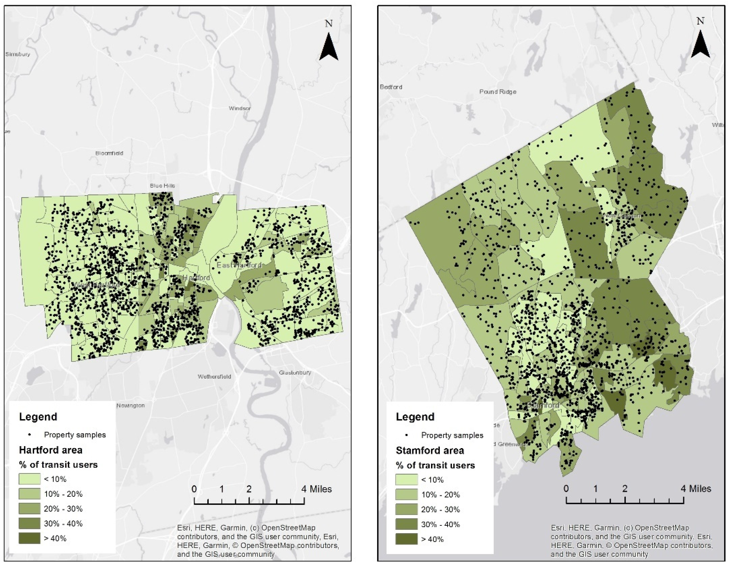
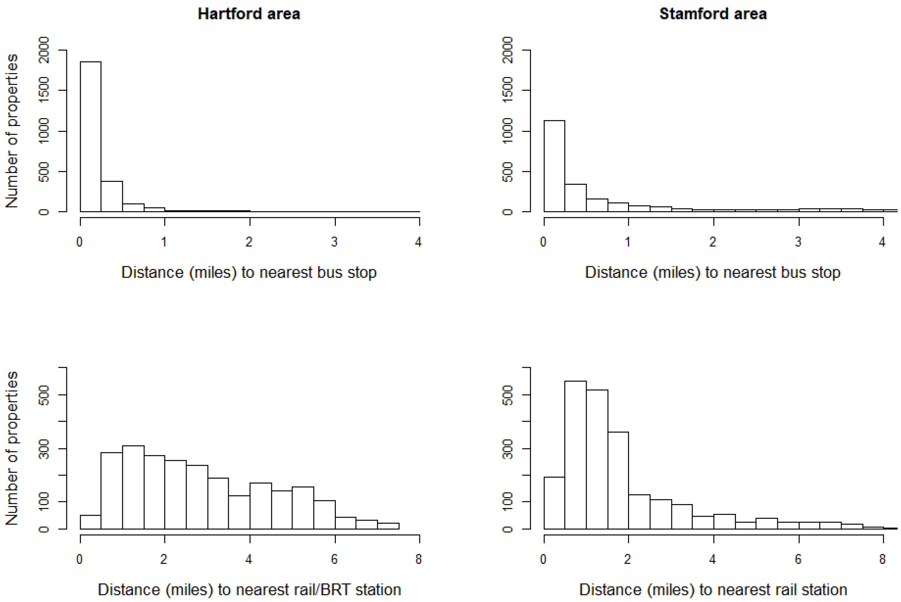
2. Study Area and Data

Connecticut (CT) is located in the northeastern United States with a population of 3.57 million [26]. It is bordered by New York, Massachusetts, and Rhode Island. Several agencies offer public transportation services in Connecticut. CTtransit and CTfastrak provide bus services throughout the state. CTfastrak is the first BRT line in the state, and it operates on dedicated busways. CTtransit and privately-operated express bus lines (including Peter Pan/Arrow Line, Collins Bus Service, DATTCO, etc.) are available for express service to Hartford. CTrail offers rail service on New Haven Line, Shore Line East, and Hartford Line. In the Hartford metro area, CTtransit operates over 30 local and 13 express bus routes. CTtransit Stamford operates 15 local bus routes [27]. The US Census Bureau estimates the percentage of people using public transportation (excluding taxicab) to work. In the state of Connecticut, southwestern towns (e.g., Greenwich, Norwalk) have the highest percentages of people relying on public transit for the daily commute. In most parts of the state, less than 5% of people use public transit to work [26]. This indicator corresponds with the availability of public transit and population density in the state. The high percentage of transit users observed in southwestern Connecticut is also attributed to the proximity to New York City.
In this study, we consider the residential properties in six cities and towns—the Hartford area includes West Hartford, Hartford, and East Hartford; the Stamford area includes Stamford, Darien, and New Canaan. Property transaction data are obtained from Redfin Data Center (www.redfin.com). Transactions made between December 2017 and November 2018 are considered to have a sufficiently large dataset and to minimize the effect of transit route changes for better reliability. Incorrect data samples (e.g., properties with 0 bedrooms, houses sold under $10,000, houses smaller than 100 square feet, etc.) are omitted from the original dataset in the analysis. In total, 2384 records in Hartford area and 2213 records in Stamford area are used in this study. Figure 1 shows the locations of property samples in the study areas and the percentage of transit users in each block group. In general, more people tend to favor transit services in the Stamford area compared with the Hartford area.
Median income and educational data for each block group are downloaded from the US Census Bureau website and are used as the input of neighborhood characteristics. The percentage of people with at least a bachelor’s degree in each block group is used as the educational attainment indicator. Transit stop information is publicly available from the General Transit Feed Specification (GTFS) file on the CTtransit and Metro North websites. Road network distances from each housing location to its nearest bus and rail/BRT stop are calculated using OpenStreetMap data [28] and ArcGIS Network Analyst. Figure 2 shows the distribution of distances from properties to their nearest stops. Comparing the results from two metro areas, we find that the bus system has better coverage in Hartford area, while access to train is much easier in Stamford area. In total, 78% of all residential property samples in Hartford area are within walking distance (a quarter mile) to a bus stop; however, only 14% of the housing samples are less than a mile from a rail/BRT station, and 38.4% of the samples are within a two-mile buffer. The scenario for Stamford area is different. While 51% of the houses are within a quarter mile to a bus stop, 33.7% of the housing samples in Stamford area are less than a mile from a train station and 73.3% of the samples are within a two-mile buffer zone.
Table 1 summarizes the descriptive statistics of the dependent and independent variables in the hedonic pricing model. The normality test shows that the original property values (dependent variable) do not have a normal distribution. A common logarithm is used on the variable “Price” to achieve a normal distribution. Note that the upper limit of median income report in the American Community Survey is $250,000. The actual median income for some block groups may be higher than this limit.

3. Methods

3.1. Hedonic Price Model

Hedonic modeling is a widely used conceptual method in evaluating housing prices. This model is based on Lancaster’s theory of consumer’s demand [29], which suggests that goods are composited by different attributes and the customers purchase these goods based on their characteristics and prices. A residential property can be regarded as a combination of base value plus different features; therefore, its value can be attributed to several factors. Hedonic modeling aims to separate the effects of these characteristics and determine the contribution of each factor [5]. In this paper, we use a hedonic price model to estimate the effects of public transportation on residential property values. A generalized form of the conceptual hedonic pricing model used in this study is:
P = f ( N ,   H ,   T , e )
where P is the sold price of a property, N is a combination of neighborhood traits (including median income and educational attainment), H is a combination of house characteristics (including square footage, number of bedrooms and baths, age of house), T is a combination of transit related variables of a house (including network distance to a nearest bus stop, and distance to nearest rail or BRT stations), and e is the error term. As mentioned above, to meet the normal distribution requirement of the dependent variable (property price), a common logarithm transformed variable log10(price) is substituted as the dependent variable in the model. Then, model (1) can be specified as a multiple regression as follows:
log 10 ( p r i c e ) = β 0 + β 1 B e d r o o m + β 2 B a t h r o o m + β 3 S i z e + β 4 A g e + β 5 M e d i a n I n c o m e + β 6 E d u A t t a i n m e n t + β 7 D i s t B u s + β 8 D i s t R a i l + ε
where β 0 is a constant term (intercept) and β 1 , ,   β 8 denote the regression coefficients of housing characteristics, neighborhood traits, and transit-related variables, described in Table 1.

3.2. Global Regression Analysis—Ordinary Least Squares

Ordinary Least Squares (OLS) is one of the most widely used regression techniques. It is a linear modeling method to model the relationships of a single response variable and related explanatory variables [30]. The theory is that the relationship between a response variable y and explanatory variable x can be expressed using a line, where y is predicted by x. The least square principle means that the sum of the squared errors of prediction of the model should be as small as possible [30]. OLS analysis is performed for the two study areas independently.
Conventional analysis methods including OLS typically use one single set of coefficients to represent the overall relationships between variables at different locations. One cannot perform a location-specific analysis with those methods. In fact, many relationships are not spatially homogeneous. Therefore, results from these methods might be biased for spatial data. Because of the spatial variation nature of real estate data, a spatial autocorrelation test is needed. Global Moran’s I is an index to measure the spatial autocorrelation of features based on their locations and values. Table 2 shows the result of spatial autocorrelation test on the residuals of the OLS model in both study areas. The Moran’s Indices and p-values show that the residuals from OLS regression are spatially clustered.

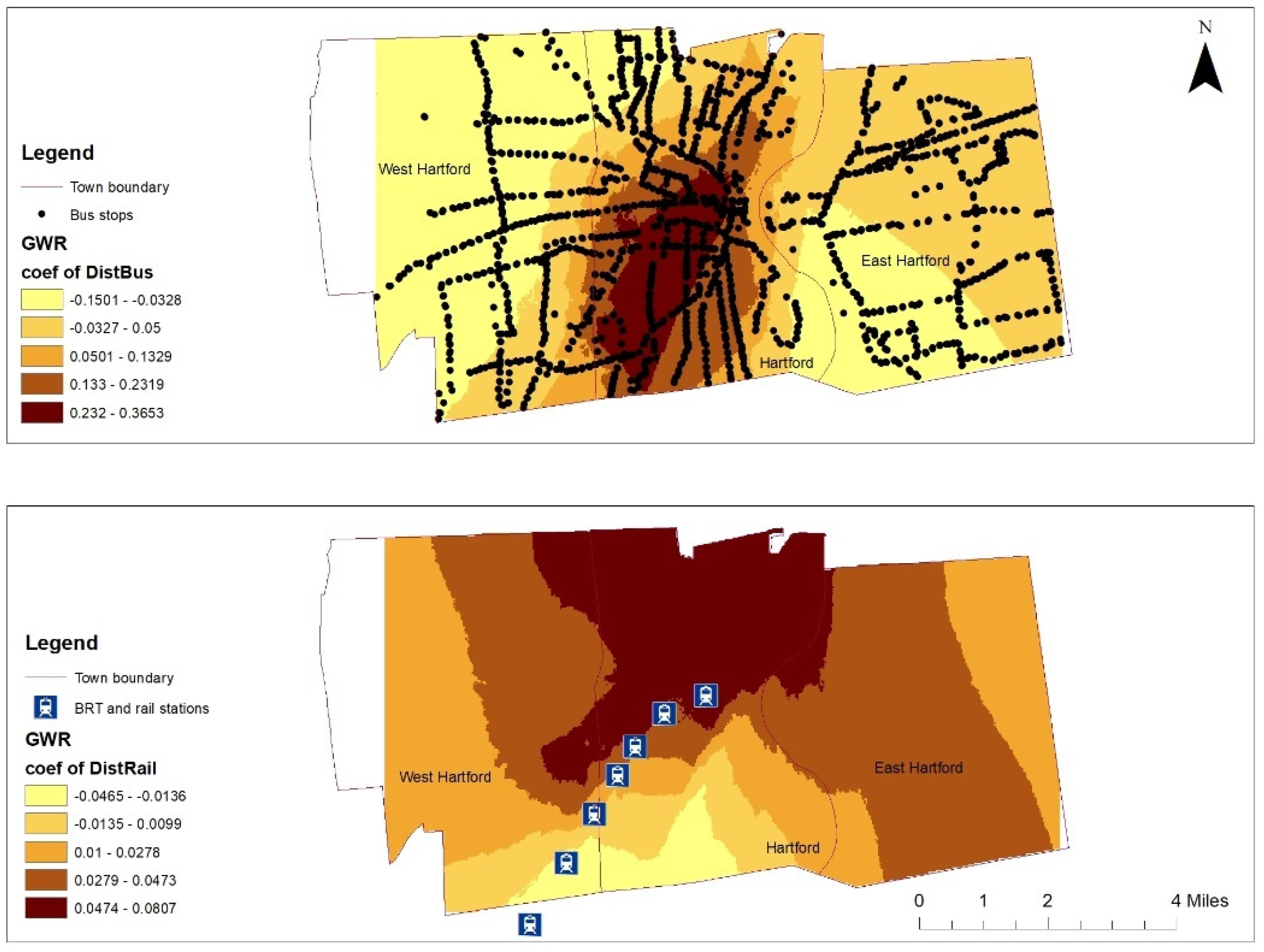
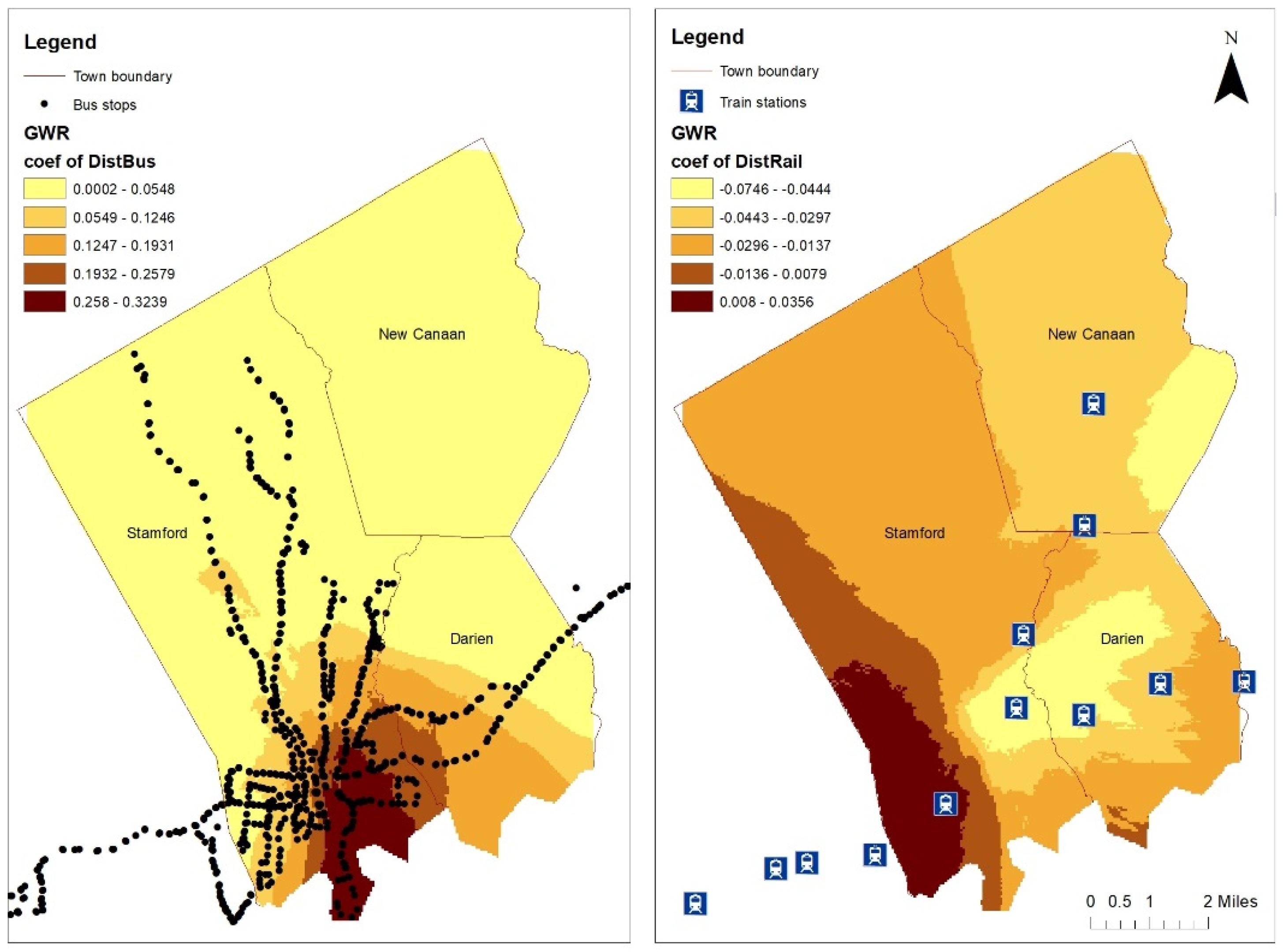
3.3. Local Regression Analysis—Geographically Weighted Regression

Geographically Weighted Regression (GWR) was proposed as a method to address the spatial dependence effect by Brunsdon et al. [31]. GWR is an extension of the OLS regression mentioned above. Given the global regression model as:
y i = β 0 +   j = 1 p x i j β j + ε i
GWR allows local parameters to be estimated based on samples within a bandwidth of the local location. The GWR model can be written as:
y i = β 0 ( u i , v i ) + j = 1 p x i j β j ( u i , v i ) + ε i
where ( u i , v i ) is the coordinates of the i th point, β 0 ( u i , v i ) is the location specific intercept, β j ( u i , v i ) is the location specific coefficient at point i , x i j is the j th variable related to β j ( u i , v i ) , p is the number of local parameters to be estimated, and ε i is the error term [32]. From both equations above, one can see that the global OLS model can be regarded as a special case of GWR model when parameters are assumed to be constant while GWR recognizes the spatial variations. For the calibration of Equation (4), it is assumed that observed data near location i have more influence in the estimation of β j ( u i , v i ) than points further away. Hence, the parameters in the GWR model are locally estimated using a weighted least squares approach, and data closer to i are weighted more than data further away [33]. Therefore, the key difference between OLS and GWR is that the coefficients in OLS are constant, while the coefficients in GWR vary with location.

4. Results and Discussion

Results from global OLS regression are shown in Table 3. In general, all the variables are statistically significant at a 5% level. The OLS model fits the data better in the Stamford area than in the Hartford area. Note that negative coefficients of ‘Distance to bus stop’ or ‘Distance to rail/BRT’ variables indicate positive impacts from the proximity to public transportation stops, and vice versa. The global regression analysis shows property value appreciation from bus services in Hartford area and from rail services in Stamford area—property values increase when distance to the nearest bus stop decreases in Hartford area, and the same is true when distance to the nearest rail station in Stamford area decreases. This estimation is consistent with the availability of the transit services in both study areas—there is a better coverage of bus stops in the Hartford area and an easier access to rail stations in the Stamford area.
Results from the GWR analysis show apparent improvement in data fitting compared with results from OLS. For Hartford area data, the adjusted R-squared is 0.6420 (OLS: 0.6021) and the AICc is −1846.42 (OLS: −1401.31). For Stamford area data, the adjusted R-squared is 0.8429 (OLS: 0.7930) and the AICc is −2861.41 (OLS: −2256.17). Therefore, GWR has better modeling performance.
In addition to estimating variable coefficients at sample locations, another advantage of GWR is that local estimates of coefficients could be made for any location in the study area, not necessarily at the locations with observed data. GWR analysis provides a continuous surface of coefficient values. This could provide complete information (exhaustive maps) to transit-oriented development policy making in both study areas. Because this study is concentrated on the impacts of proximity to public transit, only the local coefficients of the explanatory variables DistBus and DistRail from GWR analysis are shown in Figure 3 and Figure 4.
One can see that the coefficients show considerable spatial variation in both the Hartford and Stamford areas. Proximity to a bus stop has a light positive to no effect in East Hartford. In the downtown and southern parts of Hartford, this variable mostly has negative impacts on property values. Light positive impacts from bus stops appear in West Hartford with the coefficient ranging from −0.15 to −0.03. The effect from rail/BRT is more spatially uniform compared with that from bus. The local coefficients associated with variable DistRail range from −0.0465 to 0.0807, while for buses they range from −0.1501 to 0.3653 (Figure 3). Slight positive impacts from rail/BRT occur in the south end of Hartford, and negative impacts occur in other places, especially the north. The difference between the impacts from DistBus and DistRail should be caused by the service characteristics in Hartford area. As mentioned before, bus stops have good spatial coverage in the Hartford area, while access to rail/BRT stations is not as easy as in Stamford area. It should also be noted that the BRT system in the Hartford area (CTfastrak) was launched in March 2015, and the rail line (Hartford Line) began service in August 2018. It usually takes several years for rail and BRT transit infrastructure to mature and have an impact on property values in the surrounding areas. A study in Los Angeles also found that multi-family residential properties showed a large premium when the rail transit is in a mature stage [7]. The relatively short service history also contributes to the lower impact of rail/BRT service observed in the Hartford area.
Patterns in the Stamford area are different from what we found in the Hartford area. The DistBus variable shows no to slight negative impact on property values in the north Stamford area and New Canaan because of limited bus service in this area. Stronger negative impacts are found in and around downtown Stamford. In contrast, results show that distance to nearest rail station has positive effects on residential property values in most part of the Stamford area (Figure 4). This positive effect is more prominent in areas with rail stations (e.g., Darien and south New Canaan). Light negative effect occurs in downtown Stamford.
It is worth noting that there are substantial differences of income level within the two chosen study areas. According to the US Census 2019 reports [34], West Hartford sees a much higher per capital income ($56,692) than Hartford ($21,163) and East Hartford ($29,015); the per capita income for Darien ($116,564) and New Canaan ($118,833) are significantly higher than that of Stamford ($55,049). The regional differences within the study areas may also contribute to the non-uniform results.

5. Conclusions

In this study, hedonic modeling implemented by OLS and GWR models is employed to study the impacts of proximity to public transit stops on residential property values in two areas in Connecticut—the Hartford area (Hartford–West Hartford–East Hartford) and the Stamford area (Stamford–Darien–New Canaan). These two chosen study metro areas have their respective unique traits in socioeconomic status and public transport availability. In total, sales data of 2384 properties in the Hartford area and 2213 properties in the Stamford area are used in this study. Our results indicate that the impact of the proximity to a rail system on property values is overall positive in the Stamford area, while the effect from rail/BRT is smaller in the Hartford area. The reason may be that the Stamford area has a better network coverage of rail system compared with the Hartford area. The service provided by the rail/BRT in the Hartford area did not significantly improve the public transportation availability in this area. The smaller observed impact could also be due to the relative youth of the BRT and CTrail systems. The impact of distance to nearest bus stop on property values varies in the Hartford area, while it is negative in the Stamford area.
Spatial data (e.g., housing value data in this study) commonly have spatial dependence effect, which is ignored by nonspatial models, as revealed by the spatial autocorrelation of global regression OLS model residuals. Therefore, spatial regression (e.g., GWR, spatial lag models, spatial error models) should be considered. Compared with OLS (or global regression model in general), the major advantage of GWR is that it takes local spatial relationships into consideration. By considering local weights, GWR could help capture more details from the data at local scale. In both of our study areas, the GWR model produced a better data fitting with lower AICc and higher adjusted-R2 values compared with the OLS model. This study shows that rail service tends to increase residential property prices in large parts of our study areas. Such a result may provide guidance for future transit service development in Connecticut and other states with similar socioeconomic characteristics. The effect is more prominent in the Stamford area where the transit usage rate is relatively high.
The analysis could be improved with more detailed information in future studies. For example, more neighborhood attributes (urban greenery, crime rate, school districts, etc.) and property physical characteristics (whether the property has a pool, solar energy panel, etc.) may be considered for better model fitting. More robust measures of access to transit services, such as the Transit Opportunity Index [35,36] might be used as indicators of service availability. Given the relatively short service history of the BRT and Hartford Line in the Hartford area, there is a lack of housing turnover data to measure the impact from these services. Future work could focus on a pre/post comparison and time series analysis of the real estate market to investigate the effects of CTfastrak and CTrail with long term data.

Author Contributions

Conceptualization, Bo Zhang and Nicholas Lownes; methodology, Bo Zhang, Weidong Li, and Chuanrong Zhang; formal analysis, Bo Zhang; data curation, Bo Zhang; writing—original draft preparation, Bo Zhang; writing—review and editing, Weidong Li, Nicholas Lownes, and Chuanrong Zhang; visualization, Bo Zhang. All authors have read and agreed to the published version of the manuscript.

Funding

This research received no external funding.

Institutional Review Board Statement

Not applicable.

Informed Consent Statement

Not applicable.

Data Availability Statement

Publicly available datasets were analyzed in this study. These data can be found at: www.census.gov; www.redfin.com; planet.openstreetmap.org.

Acknowledgments

We thank the anonymous reviewers for their comments and suggestions. We also thank Awanti Acharya and Rob Smith for their help with data acquisition and useful discussion. Map data used in road network distance calculation copyrighted OpenStreetMap contributors and available from https://www.openstreetmap.org.

Conflicts of Interest

The authors declare no conflict of interest.

References

  1. Federal Transit Administration. Federal Transit Administration Annual Report on Funding Recommendations: Fiscal Year 2020. 2019. Available online: https://www.transit.dot.gov/funding/grant-programs/capital-investments/annual-report-funding-recommendations (accessed on 19 December 2019).
  2. FTA Office of Budget and Policy. 2017 National Transit Summary and Trends. 2018. Available online: https://www.transit.dot.gov/ntd/annual-national-transit-summaries-and-trends (accessed on 19 December 2019).
  3. Ransom, M.R. The effect of light rail transit service on nearby property values: Quasi-experimental evidence from Seattle. J. Transp. Land Use 2018, 11. [Google Scholar] [CrossRef]
  4. Cervero, R.; Duncan, M. Transit’s Value-Added Effects: Light and Commuter Rail Services and Commercial Land Values. Transp. Res. Rec. 2002, 1805, 8–15. [Google Scholar] [CrossRef]
  5. Xiao, Y. Hedonic Housing Price Theory Review. In Urban Morphology and Housing Market; Xiao, Y., Ed.; Springer: Singapore, 2017; pp. 11–40. [Google Scholar]
  6. D’Acci, L. Quality of urban area, distance from city centre, and housing value. Case study on real estate values in Turin. Cities 2019, 91, 71–92. [Google Scholar] [CrossRef]
  7. Zhong, H.; Li, W. Rail transit investment and property values: An old tale retold. Transp. Policy 2016, 51, 33–48. [Google Scholar] [CrossRef]
  8. Pilgram, C.A.; West, S.E. Fading premiums: The effect of light rail on residential property values in Minneapolis, Minnesota. Reg. Sci. Urban Econ. 2018, 69, 1–10. [Google Scholar] [CrossRef]
  9. Bowes, D.R.; Ihlanfeldt, K.R. Identifying the Impacts of Rail Transit Stations on Residential Property Values. J. Urban Econ. 2001, 50, 1–25. [Google Scholar] [CrossRef]
  10. Gallo, M. The Impact of Urban Transit Systems on Property Values: A Model and Some Evidences from the City of Naples. J. Adv. Transp. 2018. [Google Scholar] [CrossRef]
  11. Martínez, L.M.; Viegas, J.M. Effects of Transportation Accessibility on Residential Property Values: Hedonic Price Model in the Lisbon, Portugal, Metropolitan Area. Transp. Res. Rec. 2009, 2115, 127–137. [Google Scholar] [CrossRef]
  12. Li, Z. The impact of metro accessibility on residential property values: An empirical analysis. Res. Transp. Econ. 2018, 70, 52–56. [Google Scholar] [CrossRef]
  13. Pan, Q. The impacts of an urban light rail system on residential property values: A case study of the Houston METRORail transit line. Transp. Plann. Technol. 2013, 36, 145–169. [Google Scholar] [CrossRef]
  14. Pan, Q.; Pan, H.; Zhang, M.; Zhong, B. Effects of Rail Transit on Residential Property Values: Comparison Study on the rail transit Lines in Houston, texas, and Shanghai, China. Transp. Res. Rec. 2014, 2453, 118–127. [Google Scholar] [CrossRef]
  15. Perdomo Calvo, J.A. The effects of the bus rapid transit infrastructure on the property values in Colombia. Travel Behav. Soc. 2017, 6, 90–99. [Google Scholar] [CrossRef] [Green Version]
  16. Cervero, R.; Kang, C.D. Bus rapid transit impacts on land uses and land values in Seoul, Korea. Transp. Policy 2011, 18, 102–116. [Google Scholar] [CrossRef] [Green Version]
  17. Mulley, C.; Ma, L.; Clifton, G.; Yen, B.; Burke, M. Residential property value impacts of proximity to transport infrastructure: An investigation of bus rapid transit and heavy rail networks in Brisbane, Australia. J. Transp. Geogr. 2016, 54, 41–52. [Google Scholar] [CrossRef] [Green Version]
  18. Ma, L.; Ye, R.; Titheridge, H. Capitalization Effects of Rail Transit and Bus Rapid Transit on Residential Property Values in a Booming Economy: Evidence from Beijing. Transp. Res. Rec. 2014, 2451, 139–148. [Google Scholar] [CrossRef]
  19. Stokenberga, A. Does Bus Rapid Transit Influence Urban Land Development and Property Values: A Review of the Literature. Transp. Rev. 2014, 34, 276–296. [Google Scholar] [CrossRef]
  20. Shen, Q.; Xu, S.; Lin, J. Effects of bus transit-oriented development (BTOD) on single-family property value in Seattle metropolitan area. Urban Stud. 2018, 55, 2960–2979. [Google Scholar] [CrossRef]
  21. Wang, Y.; Potoglou, D.; Orford, S.; Gong, Y. Bus stop, property price and land value tax: A multilevel hedonic analysis with quantile calibration. Land Use Policy 2015, 42, 381–391. [Google Scholar] [CrossRef] [Green Version]
  22. Song, Y.; Knaap, G. New urbanism and housing values: A disaggregate assessment. J. Urban Econ. 2003, 54, 218–238. [Google Scholar] [CrossRef]
  23. Des Rosiers, F.; Thériault, M.; Voisin, M.; Dubé, J. Does an Improved Urban Bus Service Affect House Values? Int. J. Sustain. Transp. 2010, 4, 321–346. [Google Scholar] [CrossRef]
  24. Yang, L.; Zhou, J.; Shyr, O.F.; Huo, D. Does bus accessibility affect property prices? Cities 2019, 84, 56–65. [Google Scholar] [CrossRef]
  25. US Census Bureau, Top 10 Metro Areas by Percentage of Workers Who Commute by Public Transportation. Available online: https://www.census.gov/library/visualizations/interactive/public-transport.html (accessed on 28 November 2019).
  26. US Census Bureau, 2013–2017 American Community Survey 5-Year Estimates. Available online: https://www.census.gov/programs-surveys/acs (accessed on 17 December 2019).
  27. CTtransit, about Cttransit—Connecticut DOT-Owned Bus Service. Available online: https://www.cttransit.com/about (accessed on 6 December 2019).
  28. OpenStreetMap Contributors. Planet Dump Data File of 25 March 2019. Available online: https://planet.openstreetmap.org (accessed on 30 March 2019).
  29. Lancaster, K.J. A New Approach to Consumer Theory. J. Political Econ. 1966, 74, 132–157. [Google Scholar] [CrossRef]
  30. Hutcheson, G. Ordinary Least-Squares Regression. In The SAGE Dictionary of Quantitative Management Research; Moutinho, L., Hutcheson, G., Eds.; SAGE Publications: London, UK, 2011; pp. 224–228. [Google Scholar]
  31. Brunsdon, C.; Fotheringham, A.S.; Charlton, M.E. Geographically Weighted Regression: A Method for Exploring Spatial Nonstationarity. Geogr. Anal. 1996, 28, 281–298. [Google Scholar] [CrossRef]
  32. Fotheringham, A.S.; Charlton, M.E.; Brunsdon, C. Geographically Weighted Regression: A Natural Evolution of the Expansion Method for Spatial Data Analysis. Environ. Plann. A 1998, 30, 1905–1927. [Google Scholar] [CrossRef]
  33. Fotheringham, A.S.; Brunsdon, C.; Charlton, M. Geographically Weighted Regression: The Analysis of Spatially Varying Relationships; Wiley: Chichester, UK, 2002. [Google Scholar]
  34. US Census Bureau, QuickFacts Data Access Tool. Available online: https://www.census.gov/data/data-tools/quickfacts.html (accessed on 27 November 2020).
  35. Bertolaccini, K.; Lownes, N.E.; Mamun, S.A. Measuring and mapping transit opportunity: An expansion and application of the Transit Opportunity Index. J. Transp. Geogr. 2018, 71, 150–160. [Google Scholar] [CrossRef]
  36. Mamun, S.A.; Lownes, N.E.; Osleeb, J.P.; Bertolaccini, K. A method to define public transit opportunity space. J. Transp. Geogr. 2013, 28, 144–154. [Google Scholar] [CrossRef]
Figure 1. Maps of property samples in the Hartford (left) and Stamford (right) areas with the percentage of transit users.
Ijgi 10 00044 g001
Figure 2. Number of properties by access distances to nearest transit stops in study areas.
Ijgi 10 00044 g002
Figure 3. Maps of local coefficient estimates of explanatory variables DistBus and DistRail in the Hartford area.
Ijgi 10 00044 g003
Figure 4. Maps of local coefficient estimates of explanatory variables DistBus and DistRail in the Stamford area.
Ijgi 10 00044 g004
Table 1. Summary of descriptive statistics of all variables.
Hartford AreaStamford Area
VariablesMinMeanMaxStd. devMinMeanMaxStd. dev
Price (US Dollars)10,000221,7761,015,000134,72897,221795,0967,250,000768,500
log10 (Price)45.2636.0060.28524.9885.7736.8600.3181
Bedroom13.609161.768813.292191.4026
Bathroom12.06610.50.902612.669131.4031
Size (ft2) 1450202687781027368269011,6151759
Price per square foot ($)10.96115.39482.8052.8363.01290.971809.78131.44
Age (years)072.4532630.42054.1131832.58
Median income ($)12,52874,484250,00047,18813,542134,724250,00067,680
Education attainment (%)037.1290.7927.232.4460.5095.4919.99
Distance to bus stop (mi)0.00010.19122.27950.21320.00010.81897.67931.3255
Distance to rail/BRT (mi)0.08462.85247.30781.69670.04221.81648.80591.5181
1 100 ft2 ≈ 9.29 m2; 1 mi ≈ 1.61 km.
Table 2. Measures of spatial autocorrelation for the OLS residuals.
Hartford AreaStamford Area
Moran’s Index0.4221650.431365
Expected Index−0.000420−0.000452
Variance0.0000890.000151
z-score44.81282535.183734
p-value0.0000000.000000
Table 3. Summary of ordinary least squares (OLS) regression results.
Hartford Area 1Stamford Area 2
VariablesCoef.tVIFCoef.tVIF
Intercept4.720336282.0682 ***------5.137391381.7693 ***------
Bedroom0.0126953.5708 ***2.9105740.04533412.5285 ***2.7107
Bathroom0.0333404.7626 ***2.9384950.05951212.8142 ***4.468890
Size (ft2)0.00008711.9101 ***4.1437780.00004511.6787 ***4.751940
Age (years)−0.000389−2.7475 ***1.368485−0.000299−2.9569 ***3.848668
Median income ($10,000)0.0031942.1561 ***3.7120730.01353913.9894 ***2.791030
Education attainment (%)0.00574222.2352 ***3.6410460.0018287.0958 ***1.138478
Distance to bus stop (mi)−0.042203−2.0813 ***1.3760870.0135394.9088 ***1.406633
Distance to rail/BRT (mi)0.0182217.1698 ***1.368409−0.036377−15.4941 ***1.336960
*** indicates p < 0.05; 1 Hartford area: Number of Observations: 2384; R-Squared: 0.6034; Adjusted R-Squared: 0.6021; AICc: −1401.31; 2 Stamford area: Number of Observations: 2213; R-Squared: 0.7930; Adjusted R-Squared: 0.7923; AICc: −2256.17.
Publisher’s Note: MDPI stays neutral with regard to jurisdictional claims in published maps and institutional affiliations.

