Article

ArcStereoNet: A New ArcGIS® Toolbox for Projection and Analysis of Meso- and Micro-Structural Data

1
Department of Biological, Geological and Environmental Sciences, University of Catania, Corso Italia, 57, 95129 Catania, Italy
2
Department of Earth Sciences, University of Milano, Via Mangiagalli, 34, 20133 Milan, Italy
3
School of Geosciences, University of Aberdeen, Aberdeen AB24 3UE, UK
*
Author to whom correspondence should be addressed.
ISPRS Int. J. Geo-Inf. 2021, 10(2), 50; https://0-doi-org.brum.beds.ac.uk/10.3390/ijgi10020050
Submission received: 30 November 2020 / Revised: 8 January 2021 / Accepted: 23 January 2021 / Published: 26 January 2021
(This article belongs to the Special Issue Application of Geology and GIS)

Abstract

:
ArcStereoNet is a new ArcGIS® based toolbox for stereographic projections that we implement here using Python 2.7 programming language. The reason to develop another stereographic projection package arises from the recent use of Python as an exclusive programming language within the ArcGIS® environment. This permits a more flexible approach for the development of tools with very intuitive GUIs, and also allows the user to take full advantage of all potential GIS mapping processes. The core of this new projections toolbox is based on the capability to easily apply and compare most of the commonly used statistical methods for cluster and girdle analysis of structural data. In addition to the well-known Fisher, K-means, and Bingham data elaborations, a completely new algorithm for cluster analysis and mean vector extraction (Mean Extractor from Azimuthal Data), was developed, thereby allowing a more reliable interpretation of any possible structural data distribution. Furthermore, as in any other GIS platform, users can always precisely correlate each single projected data point with the corresponding geographical/locality position, thereby merging or subdividing groups of structural stations with a simple selection procedure. ArcStereoNet also creates rose diagrams, which may be applied not only to fault/joint planes orientation data, but also for the analysis of 2D microstructural fabric parameters. These include geometrical datasets derived from the minimum bounding approach as applied to vectorized grains in thin sections. Finally, several customization settings ensure high-quality graphic outputs of plots, that also allow easy vector graphics post-processing.

1. Introduction

Structural geology, geotechnics, crystallography, and petrography as well as other geoscientific disciplines have always had the necessity to process large amounts of three-dimensional data (e.g., foliations, fault planes, joints, crystallographic orientations, and so on) that are used to extrapolate statistically meaningful quantitative parameters [1,2,3,4,5,6,7,8,9,10]. The equal-angle (a.k.a. ‘Wulff net’) and the equal-area (a.k.a. ‘Schmidt net’) azimuthal projections, generally referred to as stereoplots or stereonets, are powerful graphical tools portraying 3D orientation data in two dimensions, thus, simplifying their interpretation [11,12,13]. Although in the common geological language the term, ‘stereographic projections’ is often used to generically indicate both equal-area and equal-angle azimuthal projections, formally it should be used only to refer to the latter [14,15].
Such projection types allow the angles between lines and planes to be determined, but the relative geographical coordinates of such data in real space (e.g., rock volume) is lost [16]. Consequently, the main issue regarding the use of stereonets is linked to the loss of spatial information of the projected data, for example the relative geographical position between two families of foliations, or the spatial relationship between minerals observed in the same thin section [17].
Several pieces of software have recently been developed for the digital and semi-automatic realisation of stereoplots, such as Rick Allmendinger’s Stereonet [18], Orient [19,20,21], or Dips® by Rocscience Inc. Some of these programmes include a huge number of useful tools, such as those for statistical analysis, for rotation and transformation functions, as well as for kinematic analysis or stress field orientation analysis. However, most programmes, with the exception of Orient, do not include geospatial analysis features and cannot, therefore, effectively link the orientation data with its corresponding spatial information and geological database. Over the years, several authors have tried to solve this problem by designing stereoplots software or ‘add-ins’ to specifically exploit the geospatial analysis functionalities running on well-known GIS platforms such as ArcGIS® or QGIS®. Unlike ArcGIS®, QGIS® is distributed with an open source license, therefore, plugins development and sharing within the users’ community is highly encouraged. Thus, a lot of examples of structural geology and orientation data analysis plugins for QGIS® can be found and downloaded online. Some of the best-known plugins include qgSurf [22] and GeoTrace [23], both coded in Python.
Within the ArcGIS® environment, Knox-Robinson and Gardoll [17] were the first to implement a stereonet plotting functionality for ArcView 3.0 GIS (an ESRI predecessor of modern ArcMap®), thus, becoming the forerunners of such types of tools. With the development of ArcMap®, compatible toolbars and further add-ins were designed such as the Export Toolbox [24], written in Visual Basic for Applications (VBA), that integrated a spatial averaging routine in ArcMap® 8.2. The more recent OATools [25] is an ArcMap® add-in (for versions 10.2 and 10.3), always written in Visual Basic.NET (VB.NET) using Microsoft Visual Studio (2010) with ArcObjects, a developer kit for ArcGIS® for the definition of the Graphical User Interface (GUI). This last add-in combines GIS functionalities with orientation and statistical analysis such as the creation of density distribution diagrams and the calculation of mean vectors and fold axes.
In this scenario, we introduce here ArcStereoNet (ASN), a new Python-toolbox, compatible with the latest distributions of ArcMap® (versions 10.1+), that merges the main ArcGIS® features with the semi-automatic realisation of stereoplots. It takes as input the orientation data (linear and planar features in table format) imported or created inside ArcMap®, taking advantage of its built-in functionalities of data storage and managing. In such a way, the users can at any time, within their GIS project, precisely visualise the plotted data together with the corresponding geographical/locality position. The main ASN features also include the extrapolation of statistical parameters, the application of density contour functions and the creation of rose diagrams. Moreover, the toolbox encompasses a considerable number of plot personalisation parameters that ensure high-quality publication-ready graphics, or that can be further modified with image editing software, thanks to the supported vector image output formats.
The purpose of this work is to provide a tool capable of seamlessly combining and filling the gap between geological spatial orientation data and their georeferenced position, without losing valuable information. Moreover, by including a collection of statistical functionalities quickly applicable within ArcMap® itself, ASN avoids the use of several software packages when working with oriented georeferenced data. We provide a comparison between such statistical analyses by taking a field structural dataset from folds exposed in the Macduff area of NE Scotland as a case study. In this work, we also show how ArcMap® equipped with ASN can be a valuable instrument for the simultaneous study of structural oriented data from mesoscale to microscale, using the geo and petro-structural data collected within the Palmi Shear Zone [4,26] as a practical operative example.

2. Methods

ArcMap® takes advantage of a Python 2.7.x version, installed with the software itself, to access and manipulate geo-databases and automatize various internal processes. Expert users can run Python commands directly from the Python console. Nonetheless, ArcGIS® provides various ‘ready-to-run’ toolboxes, that can also be chained together with custom Python scripts in order to realise personalised executables (i.e., Model Builder) [2,27,28,29]. In a recent addition, ArcGIS® allows coding of fully customised toolboxes, namely ‘Python-toolboxes’, by means of the arcpy library.
ASN (available as Supplementary Material—S1) is a Python-toolbox capable of realising lower-hemisphere azimuthal projections and rose diagrams starting from oriented data, thanks to the implementation of an external Python library (i.e., mplstereonet), developed within an opensource Python project [30]. This library is based on Matplotlib, a well know external Python graphics package used for application development, interactive scripting, and publication-quality image generation across user interfaces and operating systems [31]. ASN also takes advantage of NumPy, another external Python library useful for scientific and technical computing [32] and several modules within the Python Standard Library such as ctypes, os, subprocess, sys, and more. Since ASN is a Python-toolbox, it has a fully ArcGIS®-supported GUI; users that habitually utilise ArcGIS® toolboxes will notice that the GUI is very similar to that of any other ArcGIS® tool.
The toolbox contains three different tools: ‘Stereoplots’, ‘Rose Diagrams’, and ‘Graph to Hyperlink’. Starting from oriented data, imported or created inside ArcMap® as an ESRI shapefile, ASN can carry out stereonet- (‘Stereoplots’ tool) or rose diagram- plotting (‘Rose Diagrams’ tool) of selected records, stored within the corresponding attribute table (Figure 1). The ‘Graph to Hyperlink’ tool is useful to connect the realised plots with the geographic position of the plotted data, via hyperlink.
The ‘Stereoplots’ tool requires the following inputs: the orientation data shapefile as well as four fields within its attribute table (see Figure 1b), which contains respectively azimuthal values, inclination values, measurement sampling methods (RHR, Dip direction/Dip, etc.), and feature types. To get the most out of ASN, it is recommended to rename these four fields as follows:
  • Azimuth—here, azimuthal values (i.e., direction, dip direction, or trend) are stored as numeric values.
  • Dip Angle or Dip_Angle—here, inclination values (i.e., dip or plunge) are stored as numeric values.
  • Method—here, the data format must be specified as text values, choosing from ‘RHR’, ‘DD,’ and ‘TP’ (must be written in uppercase), indicating, respectively, the following conventional sampling methods: RHR—Right Hand Rule, DD—Dip Direction/Dip, and TP—Trend-Plunge. ASN can plot together RHR and DD data, calculating the following azimuth conversion equation:
    RHR = DD 90   mod   360 ,
    with ‘mod’ indicating the modulo operator.
  • Type—Here, the user should indicate the feature type as text values (e.g., ‘Main Foliation’, ‘Stretching Lineation’, ‘Axial Plane’ etc.). Such information is not mandatory, though highly recommended. It is functional for the legend labels but also guides the toolbox to a correct grouping and graphical representation of the different types of data. When differences between facing directions of orientation data need to be highlighted (e.g., beddings with distinguishing between normal and overturned positions), this field can be populated with distinct entries (e.g., ‘Bedding normal’ and ‘Bedding overturned’), thus, prompting the tool to treat such data separately.
These suggested fieldnames can be written without taking care of uppercase/lowercase characters and their order in the attribute table is totally irrelevant. Other fields can also be added in the attribute table according to the users’ needs and preferences. If users follow such suggestions, the tool will automatically fill the required input boxes with the correct fieldname. Otherwise, they can still fill them manually through a drop-down menu showing all the suitable fieldnames of the given shapefile. The ‘Rose Diagrams’ tool has a simplified input fields requirement, as it only requires the Azimuth and the Type fields to be provided.
Once users have created the oriented data shapefile, they can select the portion of data that needs to be plotted, taking advantage of the various selection tools provided by ArcMap®, and then open the ASN toolbox and choose the desired tool (see Figure 1c). If users do not operate any data selection, the whole dataset will be considered.
The ‘Graph To Hyperlink’ tool requires as input the plots that have been generated with the previous tools and will create a new shapefile containing hyperlinks to such images together with their related geographic position. As a result, users can visualise the graphs popping up from a map at the corresponding latitude and longitude coordinates.

2.1. Azimuthal Projections

The ‘Stereoplots’ tool (Figure 2) is used to obtain lower hemisphere equal area or equal angle azimuthal projections showing cyclographic traces, and/or poles for the selected planar measurements, and/or points for the linear elements. The plottable orientation data can be selected through the drop-down menu of the ‘Plot Cyclographic Traces, Poles, and Vectors’ option, where it is grouped by feature type. Once added, data will be stacked inside the underlying table-like box (see Figure 2c). For each additional oriented data type, the user can fully customise its graphical appearance in stereoplot by setting parameters such as colour, shape, and size of lines and symbols. This type of ArcGIS® multivalue input system, consisting of a drop-down menu and a table-like box below, is called ‘Value Table’.
Within the ‘Stereoplots’ tool, density contour functions and statistical analysis are also available and can be accessed by expanding the ‘Contour & Statistics’ submenu (Figure 3). Two more Value Tables, named ‘Apply Contour’ and ‘Extract Mean Vectors’, respectively, will appear. Their working principles are the same as those expressed above.
The ‘Apply Contour’ Value Table allows the user to show the orientation density distribution of selected data. The tool uses a modified Kamb contour function with exponential smoothing [18] by default. However, other density contour functions such as the modified Kamb with linear smoothing, with inverse square smoothing [19], without smoothing (‘traditional’ Kamb function [33]) and ‘Schmidt’ (a.k.a. 1% method) are also available and can be chosen under the ‘Method’ column of the Value Table. Other parameters that may be customised are the standard deviation (σ), set by default to 2, and the desired contour style (filled or unfilled), colour, and transparency. By checking the underlying ‘Show Contour Colorbar’ checkbox, a colour bar linked to the density contour function will appear in the plot as well.
The ‘Extract Mean Vectors’ Value Table allows the user to calculate and show the mean vectors of the selected data, choosing between several clustering and mean vector extracting algorithms. The user is totally free to extract the mean vectors from various data types, also using different algorithms, at the same time. Other customisable parameters are the number of expected clusters for that specific data type (i.e., how many families does the user expect the orientation data types to be divided into), some specific algorithm-related parameters that will be discussed in detail in Section 2.1.1 (together with the different algorithms description), and the same graphical plotting features previously described (i.e., colour, shape, and size of lines and symbols).
The ‘Plot Customisation’ and the ‘Plotting Options’ submenus (Figure 2f,g) gather secondary parameters such as the output figure title label, the option to show a legend, the number and style of tick marks, the net type (Schmidt or Wulff), and more. A noteworthy parameter under the ‘Plotting Options’ submenu is the ‘Write Log File’ checkbox. This option can be checked to prompt the tool to compile a log text file (.txt), where some useful statistical information about the results of functions applied to data is stored. It is highly recommended that users select this if they have extracted mean vectors from plotted data and/or applied a density contour function.

2.1.1. ‘Stereoplots’ Tool Algorithms

Almost all of the algorithms used by the ‘Stereoplots’ tool to extract statistical parameters from oriented data consist of two main processes: the clustering process (i.e., a function that splits data into a user-defined number of families) and the mean vector extracting process (i.e., a function that extracts the mean azimuth and dip values from a given family of data). The ‘Extract Mean Vectors’ Value Table within the tool allows the user to choose the preferred algorithm, through the ‘Algorithm’ parameter (see Figure 3c). The available choices are labelled as: Mean Extractor from Azimuthal Data (M.E.A.D.), M.E.A.D. + Fisher, K-means, Bingham.
The M.E.A.D. algorithm acronym stands for ‘Mean Extractor from Azimuthal Data’; it is designed ex novo and presented here for the first time (see Figure 4). The arithmetic mean formula is not always functional to extract a correct mean vector from azimuthal datasets, since each oriented feature (planar or linear) is defined by a couple of values (azimuth-inclination). Moreover, a ‘wrap-around’ problem could also occur, i.e., the overlapping of the values 0 and 360 in a circumference. The M.E.A.D. algorithm deals with such mathematical issues by taking as input the orientation data expressed as a list of azimuth-dip couples (i.e., strike-dip for planar features or trend-plunge for linear features), a user-defined number of clusters and two user-controlled tolerance percentage values, ranging from 0 to 100. The azimuth-dip couples are automatically extracted by the tool from the orientation data, the required number of clusters can be set by the user through the third Value Table parameter (named ‘Number of Clusters’; see Figure 3c) and the two tolerance values can be adjusted through the fourth and fifth Value Table parameters (i.e., ‘M.E.A.D. Azimuth tolerance and ‘M.E.A.D. Inclination tolerance’). These last two parameters will be taken into consideration by the tool only if one of the M.E.A.D. or the M.E.A.D. + Fisher algorithms has been selected, otherwise they will simply be skipped during the tool execution phase.
Consequently, the M.E.A.D. clustering process tries to group data into the user-defined number of families (i.e., the ‘Number of Clusters’ parameter). Such a procedure can be divided into three subprocesses (see Figure 4):
  • Pre-clustering. In this subprocess the azimuth frequencies are calculated, then normalized in relation to their maximum value, and finally the azimuth-dip couples are sorted by normalized azimuth frequency.
  • Clustering. This an iterative subprocess, where the sorted azimuth-dip couples are analysed multiple times in order to group them together. With azimuth and dip values of the first couple representing the starting median values, each couple is compared with them and, if they do not diverge by more than a threshold value, they are grouped together and the median values are consequently refreshed. This is computed as:
    sin α i   sin α *     t 1 ;
    cos α i   cos α *     t 1 ;
    sin δ i   sin δ *     t 2 ;
    where αi and δi are the azimuth and dip values of the i-th couple, while α* and δ* are the current azimuth and dip median values, respectively. Both the sine and the cosine differences (Equations (2) and (3)) are needed for azimuth values, because a numerical value ranging from 0 to 360 can be unequivocally expressed only by considering both its sine and cosine contemporaneously. Instead, as the dip value ranges between 0 and 90, just one of its sine and cosine values is sufficient (Equation (4)). The maximum value for the azimuth threshold (t1) is 2, while for the inclination threshold (t2) it is 1, as the sine function ranges between −1 and 1 for azimuth values and between 0 and 1 for the dip values. The clustering subprocess is reiterated until no more clusters can be extracted; the remaining couples, if present, are considered as spurious. An important role here is covered by the azimuth and inclination tolerances set by the user through the corresponding Value Table parameters (Figure 3c), as the thresholds (t1 and t2) are proportional to such values. Experimental tests show that even a small variation of tolerance values can sometimes determine significant variations on the result. It is possible for the users to quickly test different tolerance values multiple times, by unchecking the ‘Store Image Output’ option (Figure 2d). In this way, they can obtain the graphical result that best suits their needs and preferences without wasting memory space. Another useful option to check is the ‘Track M.E.A.D. Behaviour’ (Figure 3d), which plots the clustered data (poles or lines) with different symbols (e.g., symbol ‘1′ for data that falls into the first cluster, ‘2′ for second cluster, no symbol for spurious data, etc.). This can be helpful to understand the actual influence of the user-controlled parameters on the clustering process and to simplify their setup (Figure 5).
  • Post-clustering. This subprocess performs a post-filtering operation, double-checking all extracted families and returning as output only the number of clusters required by the user, selecting the most populated ones. If such a number is higher than the actual number of families extracted by the clustering process, the function will return all the obtained clusters.
Results obtained by the clustering process are used as input for the mean vector extracting process (Figure 4), to calculate the average azimuth and dip values for each cluster. This is carried out by first converting the azimuth values from degrees to radians and then summing together all of their sines and cosines, respectively. Consequently, the 2-argument arctangent function is applied on such summations and the output is firstly converted back to degrees and then the modulo 360 is applied:
θ = deg arctan 2 i = 1 n sin α i ,   i = 1 n cos α i mod   360 ,
where αi represents the i-th azimuth value, expressed in radians, within the n-elements cluster and θ is the mean angle expressed in degrees. The inclination average value, instead, is calculated by applying the arithmetic mean formula, as the inclination values range from 0 to 90 and do not ‘wrap-around’. This computation is applied for each cluster obtained by the clustering process.
The M.E.A.D. + Fisher algorithm merges the M.E.A.D. clustering process with the Fisher mean vector extracting function [34] implemented within the mplstereonet package (see the mplstereonet documentation [35] for details). In addition to the mean vector(s), this function also generates three statistic parameters: The R value (i.e., the magnitude of each mean vector as a number between 0 and 1), the confidence radius (i.e., the opening angle of a small circle that corresponds to the confidence in the calculated direction), and the K value (i.e., the dispersion factor that quantifies the amount of dispersion of the given data). All these statistics will be stored in the log file if the user enables the ‘Write Log File’ option (Figure 2g). As the clustering process is still carried out by the M.E.A.D. algorithm, the two tolerance parameters will influence the result. In addition, the ‘Fisher confidence’ value (i.e., the sixth Value Table parameter; see Figure 3c) will also be taken into account during the execution stage of the tool. Such a parameter consists of a percentage value ranging from 0 to 99 (defaults to 95) that influences the above-mentioned confidence radius. A related confidence cone (or small circle), bearing an opening angle equal to the confidence radius value, will eventually be plotted on the stereoplot.
The K-means algorithm is also implemented within the mplstereonet package (see the mplstereonet documentation [35] for details) and consists of a k-means approach [36], modified for spherical measurements. As for the M.E.A.D., it includes both a clustering and a mean vector extracting processes. The main differences between these two algorithms lie within the iterative clustering function that starts from random points for the ASN K-means algorithm and from the most frequent azimuthal values for the M.E.A.D. Moreover, the K-means clustering iterative process is set up according to the required number of clusters (i.e., it is influenced by that number) while the M.E.A.D. makes use of such parameter only after the entire clustering subprocess is completed (see Figure 4). Finally, the K-means algorithm works with data expressed in matrix form and converted in spherical coordinates, unlike the M.E.A.D. algorithm that works with the sines and cosines of angular data.
As with Fisher algorithm, the Bingham algorithm derives from a well-known probability distribution on the sphere [37] implemented inside the mplstereonet package (see the mplstereonet documentation [35] for details). This function differs from the previous ones, as it does not feature a clustering process. It aims to find the best fit plane (and/or its related pole) of a ‘girdle-like’ distribution pattern (poles of planes or lines). Therefore, the ‘Number of Clusters’ parameter will be ignored during the tool execution if this algorithm has been selected. The influences of the user-controlled parameters on each algorithm are summarised in Table 1.

2.2. Rose Diagrams

The ‘Rose Diagrams’ tool is useful to generate weighted and unweighted rose diagrams. Its GUI structure (Figure 6) is very similar to the ‘Stereoplots’ tool. As noted above, the input fields are here only the Azimuth and the Type fields. The ‘Data to be plotted’ Value Table contains four parameters that may be customised (see Figure 6c). The first one (i.e., ‘Colors’) allows the user to choose the colour of the diagram bars while the others can be used to extract a specific number of mean vectors of plotted data. Any mean vector will be shown in the plot with an arrow oriented along the mean direction, the length of which is proportional to the mean resultant length (ranging between 0 and 1). While the ‘Plot Customisation’ submenu gathers more or less the same types of parameters as the ‘Stereoplots’ tool, the ‘Plotting Options’ submenu here offers some unique parameters. The ‘Mirrored Behaviour’ checkbox can be selected to show a specular rose diagram, thus, plotting both the vectors directions carried by the azimuthal data input and the corresponding opposite vectors directions (i.e., pairs of supplementary angles). Since this option makes sense only if plotted data covers a range less than or equal to 180 degrees, the tool will automatically check if such a condition is satisfied. If it is not, a warning message will pop up. Another useful additional parameter is the ‘Weighted Rose Diagram’ checkbox. If checked, the user must then indicate which field the data should be weighted to, through the drop-down menu of the input box below. The ‘Write Log File’ parameter shares the same features described for the ‘Stereoplots’ tool.

‘Rose Diagrams’ Tool Algorithms

The ‘Rose Diagrams’ tool makes use of a modified M.E.A.D. algorithm for the extraction of mean vectors. The clustering process differs from normal M.E.A.D. for the absence of the inclination tolerance parameter, here becoming meaningless. The user can still set the ‘Number of Clusters’ and the ‘M.E.A.D. Azimuth tolerance’ parameters within the ‘Data to be plotted’ Value Table (Figure 6c). The mean vector extracting process is also slightly modified. In addition to the mathematical formula at (5), which is useful to extract the mean azimuth direction (θ), the following equation is calculated for each cluster as well:
R =   i = 1 n sin α i 2 +   i = 1 n cos α i 2 ,
where αi is the i-th azimuth value within the n-elements cluster. Here, R is the mean resultant length (ranging between 0 and 1), and its value determines the length of the arrow representing the mean vector on the plot. If the ‘Mirrored Behaviour’ option is selected, the supplementary mean azimuth direction (θ’) is also computed for each cluster and R is represented on the plot as a double-headed arrow, pointing towards both mean vectors directions. If the user prompts for a weighted rose diagram, the magnitude of the selected weights must be evaluated within the calculation of the mean vectors. Therefore, Equations (5) and (6) become, respectively:
θ = deg arctan 2 i = 1 n sin α i · w i i = 1 n w i ,   i = 1 n cos ( α i ) · w i i = 1 n w i mod   360 ;
R = i = 1 n sin ( α i ) · w i i = 1 n w i 2 +   i = 1 n cos α i · w i i = 1 n w i 2 ,
with wi representing the i-th weight value associated to each azimuth value (αi) within the n-elements cluster.

2.3. Output Images

The users can save the stereoplot or rose diagram images they have produced by clicking on the ‘Output Image’ parameter present in both tools (see Figure 2d and Figure 6d) and then selecting a file path and one of the following available file extensions: ‘.png’, ‘.eps’, ‘.pdf’, ‘.pgf’, ‘.ps’, ‘.raw’, ‘.rgba’, ‘.svg’, ‘.svgz’. The resolution can be set with a DPI value ranging from 0 to 600 (200 is the default value). The image file can also be saved as a temporary file by unchecking the ‘Store Image Output’ parameter. In such a way, the tool will save a PNG file into the ArcGIS® default scratch folder and automatically open it with the default local image viewer. If the user also requires the log file, it will be saved as a temporary file and automatically opened too. These files will be deleted by ASN immediately after the user prompts for a new temporary image.
The ‘Graph To Hyperlink’ tool can be used to link the realised graphs to their related spatial positions in the map (Figure 7). Each position corresponds to the mean latitude and longitude coordinates (a.k.a. the centroid) of the dataset from which the related graph was extracted. This tool takes as input the plots as raster images and outputs a new punctual shapefile, where each record stores a graph file path and its corresponding latitude and longitude coordinates.

3. ASN Worked Examples

ASN was tested with several oriented datasets during the design phase. We here select two case studies involving the Macduff area of NE Scotland [38] and the Palmi Shear Zone of Calabria in southern Italy [4,26]. These case studies provide a comparison to showcase the various ASN statistical algorithms, and are an example of the simultaneous study of oriented structural data from the mesoscale to microscale, respectively.

3.1. Macduff Case Study: Algorithms Comparison

The geology of the Macduff area in NE Scotland forms part of the Dalradian Supergroup that is a late Pre-Cambrian to Cambrian sedimentary sequence that was subsequently deformed and variably metamorphosed during the Early–Mid Ordovician Grampian Orogeny at 475–465 Ma [39,40]. The Macduff area (UK Grid: NJ7190 6465) comprises sandstones and mudstones that originally formed deep water turbidite fans and were subsequently regionally metamorphosed to biotite facies during the Grampian Orogeny [39,40,41]. Structurally, the Macduff area is dominated by NNE-trending upright anticlines and synclines that develop at wavelengths of meters to hundreds of metres [38]. The relatively low metamorphic grade and varied lithologies allow bedding and cleavage to be readily identified around the gently-plunging folds, that are cut across and exposed by the E-W trending coastline [38,41] (Figure 8).
The dataset consists of 40 bedding measurements (see Table A1 and Table A2 in Appendix A) that were collected using a geological compass from fold limbs that were already grouped by the field investigator into two different families (i.e., west and east limbs of the NNE trending anticlines). We simulated three different ways of approaching the problem with ASN in order to extract the mean planes that best define the whole dataset. Since field investigations do not always allow an easy distinction between two or more families of data, the first two simulations ignored the data differentiation identified by the field investigator, labelling all data as generic ‘Fold limb’ (Table A1). However, the third simulation considers such user-driven data distinction from around the folds (Table A2).
For the first simulation (Figure 9), the algorithm-control parameters are set to default, except for the number of clusters. The M.E.A.D. clustering-based algorithms converge, while the K-means only share the same mean strike values with them. The Bingham algorithm confirms this result, as the best fit pole coincides with the mean cyclographic traces intersections, indicating the fold axis. The greatest difference lies in the mean dip values extracted by the K-means algorithm, which would suggest a larger interlimb angle and a more asymmetrical fold. This can be attributed to the clustering approach of K-means, which tries to ‘force’ all data to cluster into the user-defined number of clusters. Instead, the M.E.A.D. algorithm tends to assemble lower dispersion clusters, thus, excluding the spurious data. This behaviour is highly customisable by the user through the tolerance parameters, as shown in the next simulation.
The second simulation (Figure 10) highlights the influence of control parameters on the result, with particular emphasis on the M.E.A.D. inclination tolerance. Three possible average inclinations for the west-dipping fold limb are highlighted. The inclination tolerance set for M.E.A.D. + Fisher algorithm is low (i.e., 7%), and this reflects a low-dispersion cluster extraction and, consequently, a higher number of spurious data. On the other hand, a much higher inclination tolerance set for M.E.A.D. algorithm (i.e., 65%) leads to a more dispersed data clustering. The K-means algorithm result differs from the others for the same reason explained in the first simulation. A contour density function is here also applied to help visualize the different clustering approaches of the ASN algorithms. The Bingham best fit pole still coincides with the cyclographic traces intersection, highlighting the fold axis.
For the third simulation (Figure 11), the data differentiation recognised by the field investigator is considered. This is done by specifying within the Type field of the attribute table two different entries (i.e., ‘West limb of Anticlines’ and ‘East limb of Anticlines’). In such a way, a data clustering is already performed by the user at outcrop and, thus, the ‘Number of Clusters’ parameter is set to 1 for all algorithms. The most noticeable consequence is that some of the data labelled as ‘East limb’ shows supplementary strike values (e.g., 30 and 210 degrees) since data is expressed with the Right-Hand Rule (RHR) method and features a high dip value. The M.E.A.D. clustering process works with sines and cosines of azimuth values; therefore, it tends not to group together supplementary strike values (confront Equations (2) and (3)). Consequently, the single cluster required by the user only gathers the SE-dipping east limb records (i.e., the most numerous) and the extracted mean cyclographic trace shows a less steep dip value. Conversely, the K-means algorithm works with data expressed in matrix form and converted in spherical coordinates, and tries to group all east limb records within the single cluster. This leads to the extraction of a steeper dipping mean cyclographic trace.

3.2. Palmi Shear Zone Case Study: Mesostructural and Microstructural Data Comparison

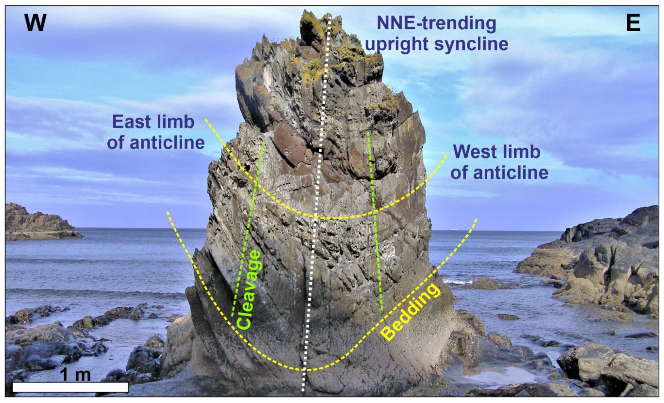
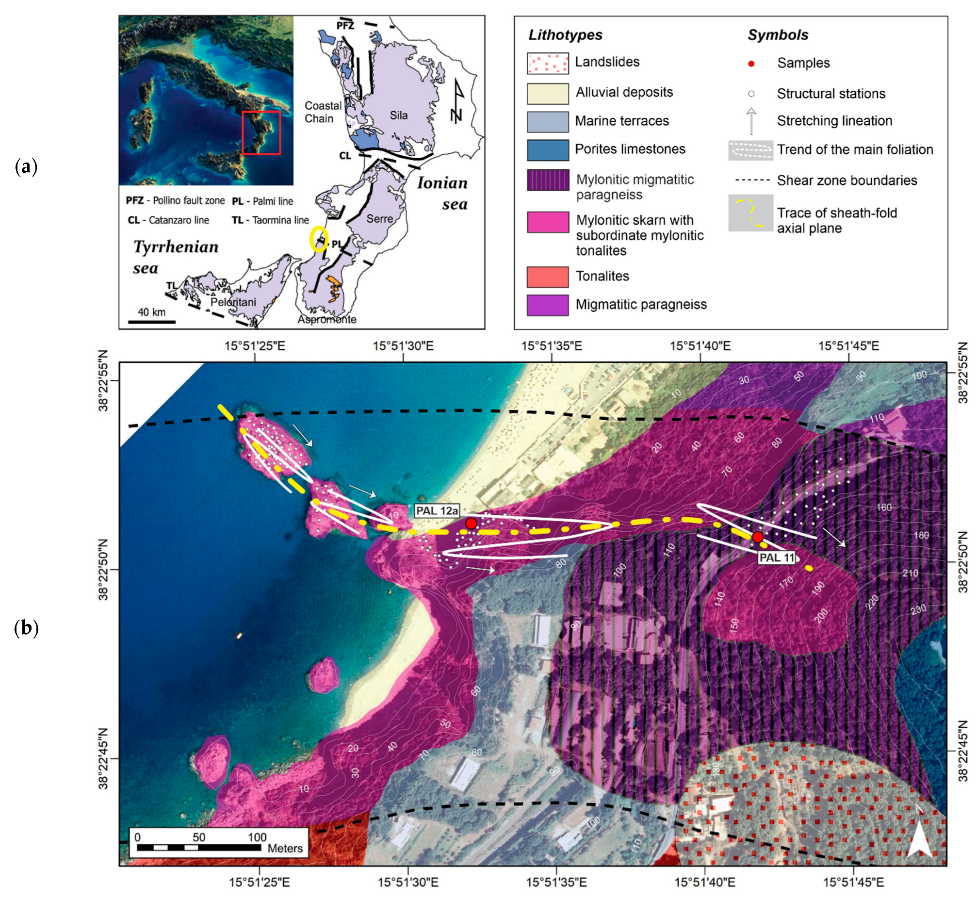
The Palmi Shear Zone (PSZ) [4,26] is a roughly E-W trending strike-slip high-strain zone, a few hundred meters in thickness, with a pervasive ductile deformation starting in the Paleocene (57 Ma [42]). The PSZ is located in the southern sector of the Calabria-Peloritani Orogen (CPO), in southern Italy [43] (Figure 12a). Here, an alternance of highly foliated calcsilicates with subordinate mylonitic migmatitic paragneiss and mylonitic tonalites occurs. The 400 m wide mylonitic horizon extends inland for about 1500 m, forming, with a prevalent subvertical foliation, along the contact between Late-Hercynian tonalites to the south and a high grade Hercynian metamorphic complex to the north (i.e., restitic paragneisses; migmatites and amphibolites [4]).
According to Ortolano et al. [4,44] and Cirrincione et al. [43], this subvertically foliated mylonitic zone can be interpreted as a northward relic fragment of the anastomosed regional-scale strike-slip system that controlled the mutual microplate movements of the Western Mediterranean realm since the Paleocene. The strike-slip movements caused the observed lateral juxtaposition of differently evolved crystalline basement terranes, such as those identified within the arcuate orogenic segment of the CPO. In particular, the PSZ is a segment of the dextral strike-slip system, known as the Palmi Line [43] (Figure 12a). This structure controlled the juxtaposition of the intensely shortened Aspromonte Massif nappe-like edifice, characterised by the presence of a pervasive Alpine re-equilibration [3,4,26,43,45] (Figure 12a), with the Serre Massif, forming a quasi-complete relic fragment of a Late-Palaezoic crustal section belonging to the original southern European palaeomargin [46].

3.2.1. Mesostructural Data Analysis

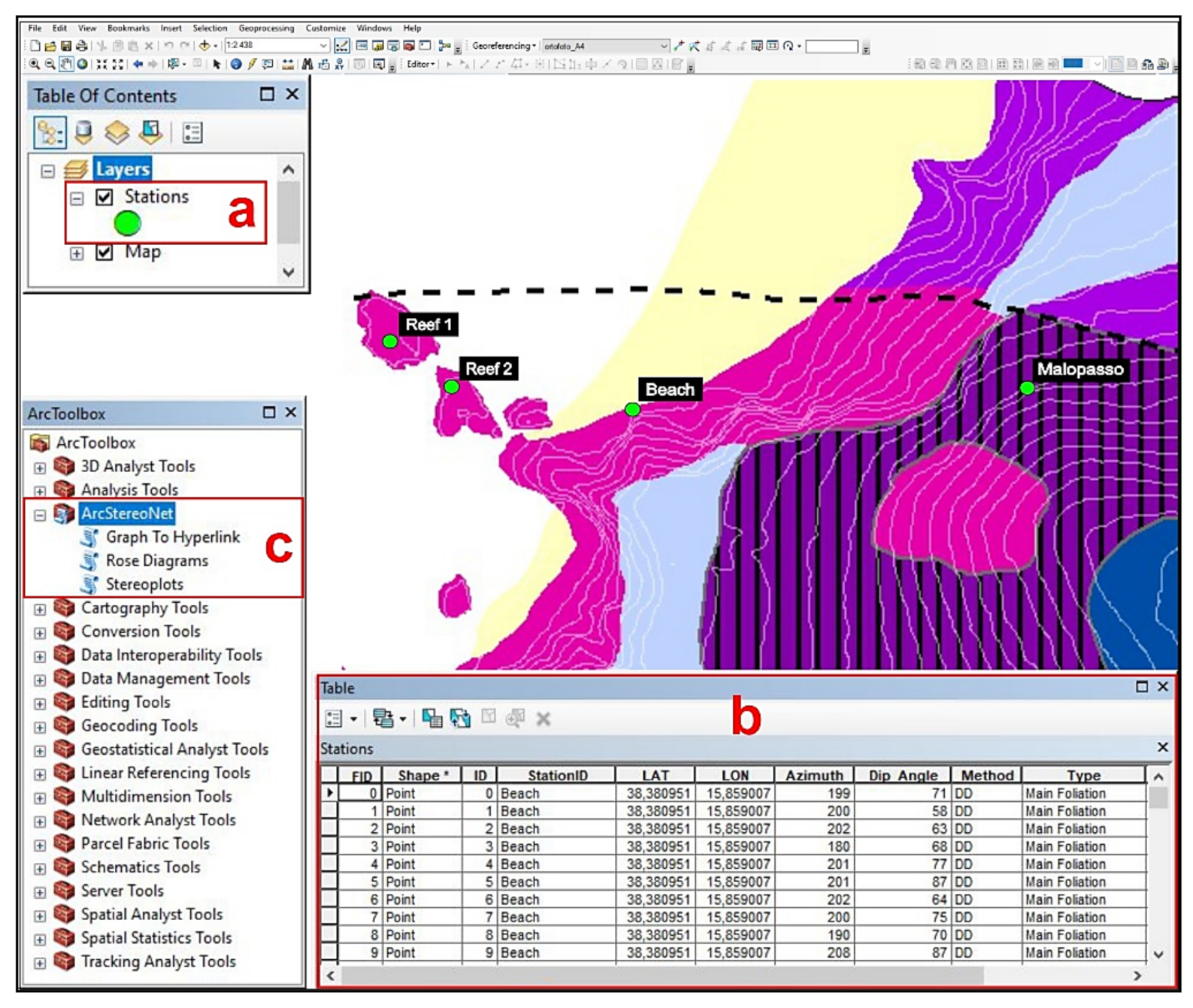
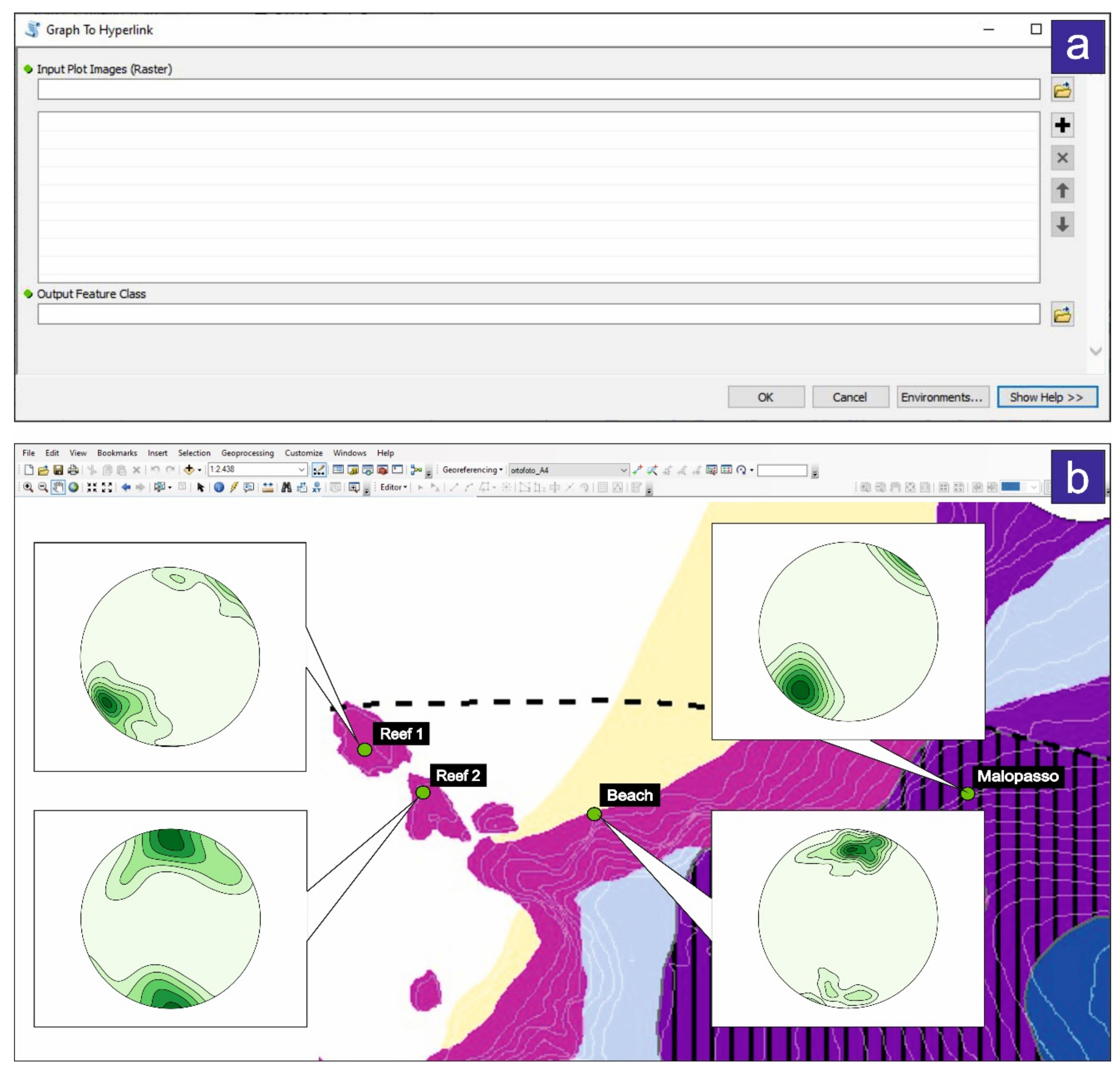
In this section, we will consider a dataset consisting of linear and planar structures measured using a geological compass during a field-survey campaign (Figure 11b). We collected structural data from four different stations (the full dataset is provided in Table S2 within the Supplementary Materials), approximately aligned along a W–E oriented direction, and named ‘Reef 1′, ‘Reef 2′, ‘Beach’, and ‘Malopasso’, respectively (Figure 1 and Figure 7).
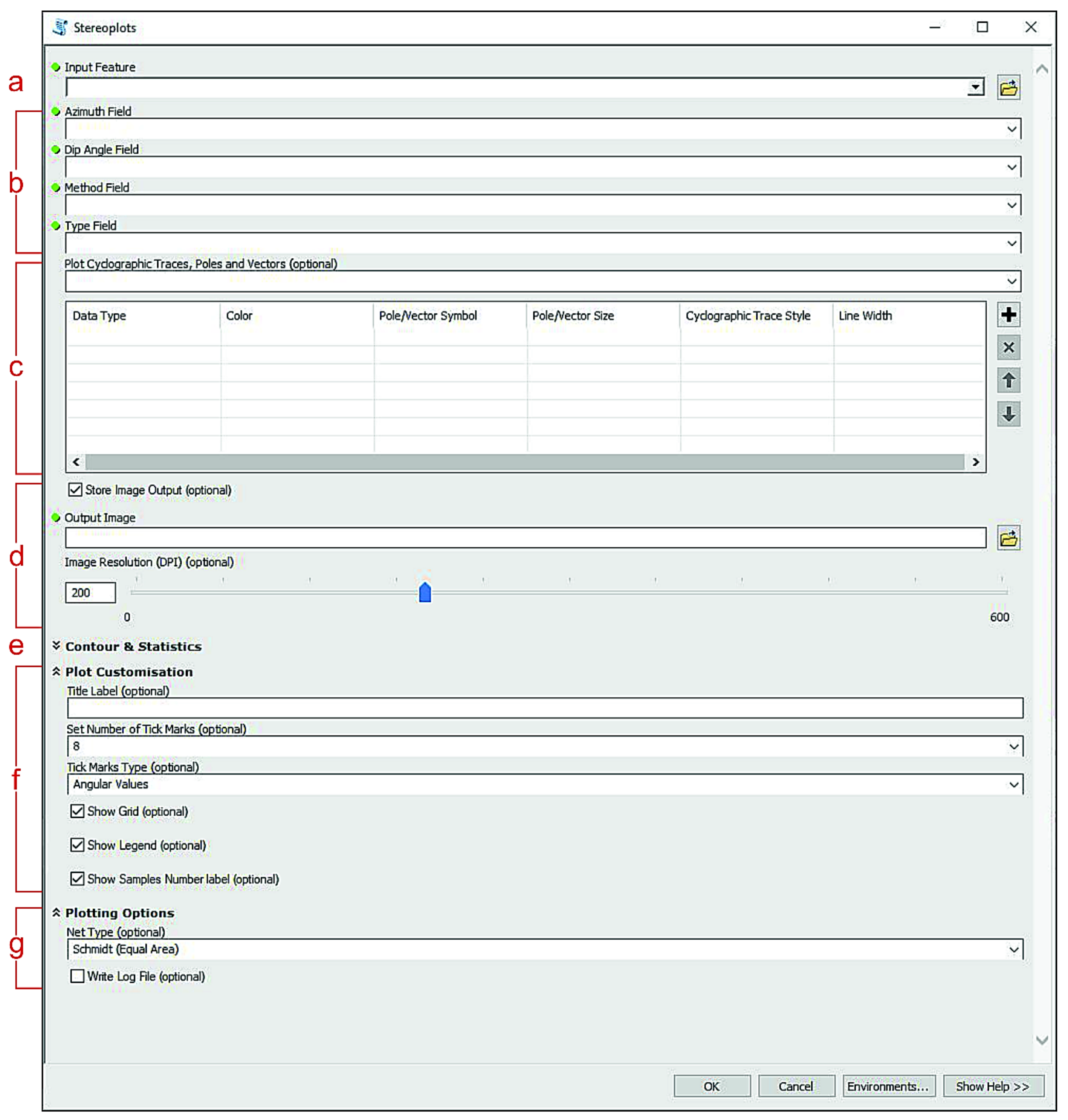
In order to test other specific characteristics of the ASN toolbox, we decided to use just the mylonitic foliations and the stretching lineations. Axes of isoclinal or sheath folds have been voluntarily excluded from the elaboration.
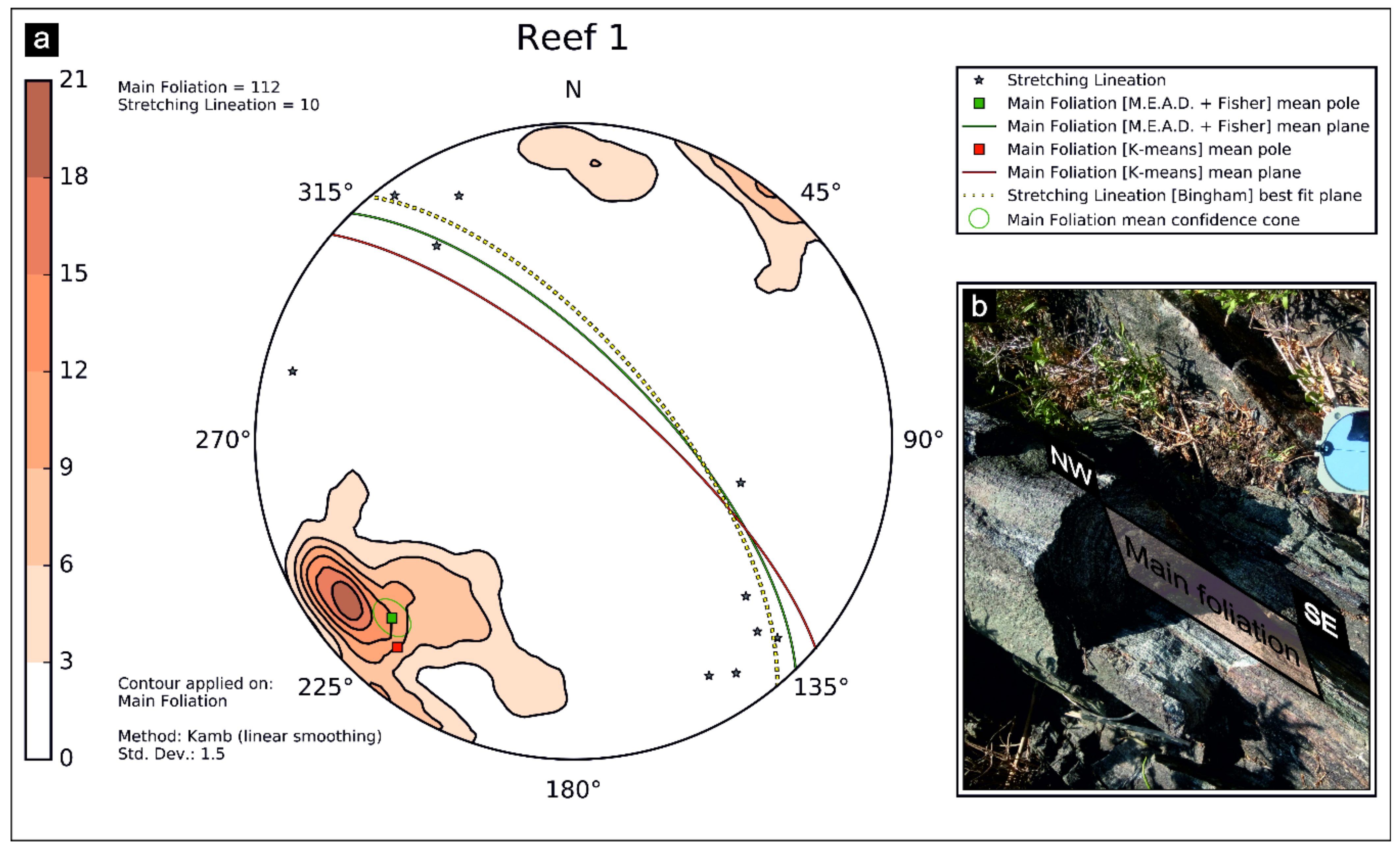
The ‘Reef 1′ station is fixed at the furthest-most sea stack with respect to the coastline. The contoured plot of poles to mylonitic foliations (n = 112; 
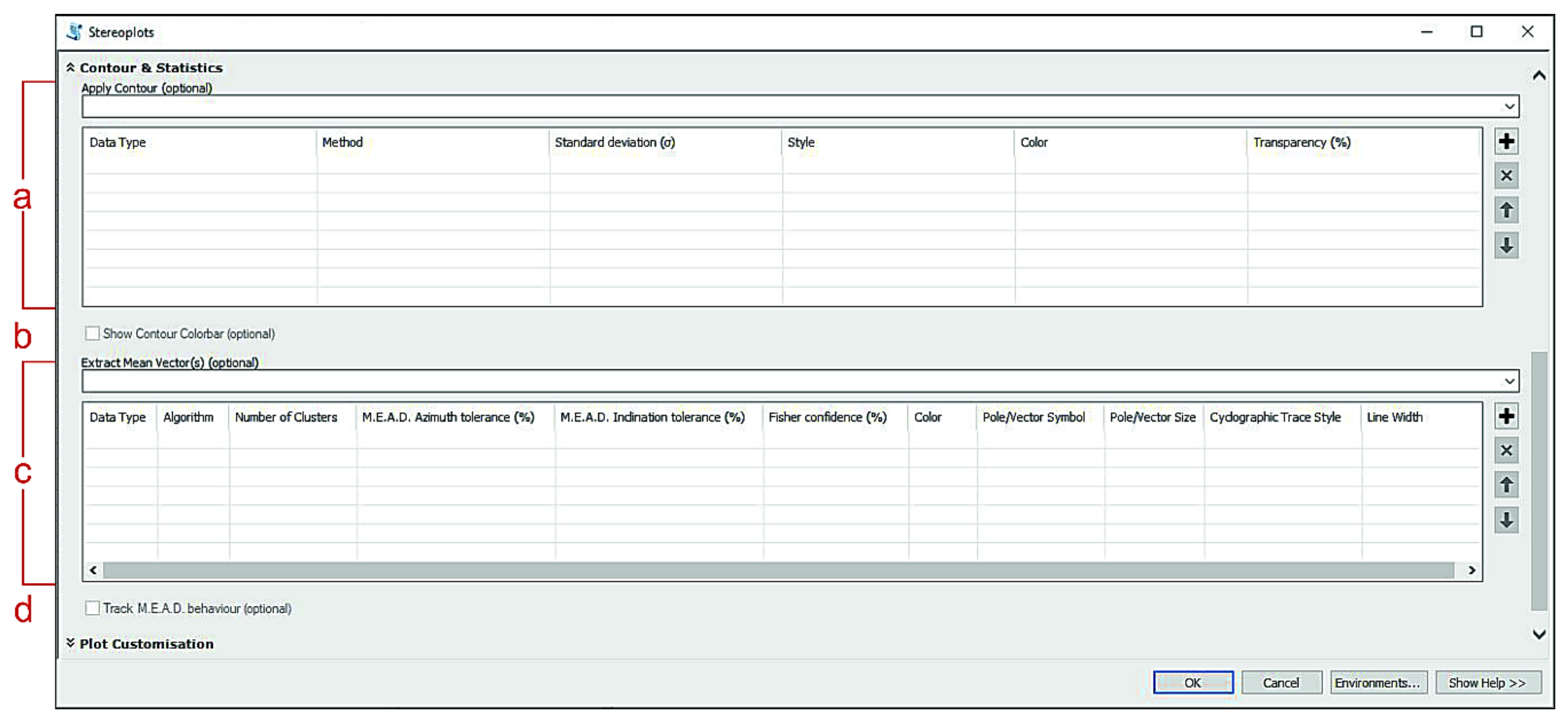
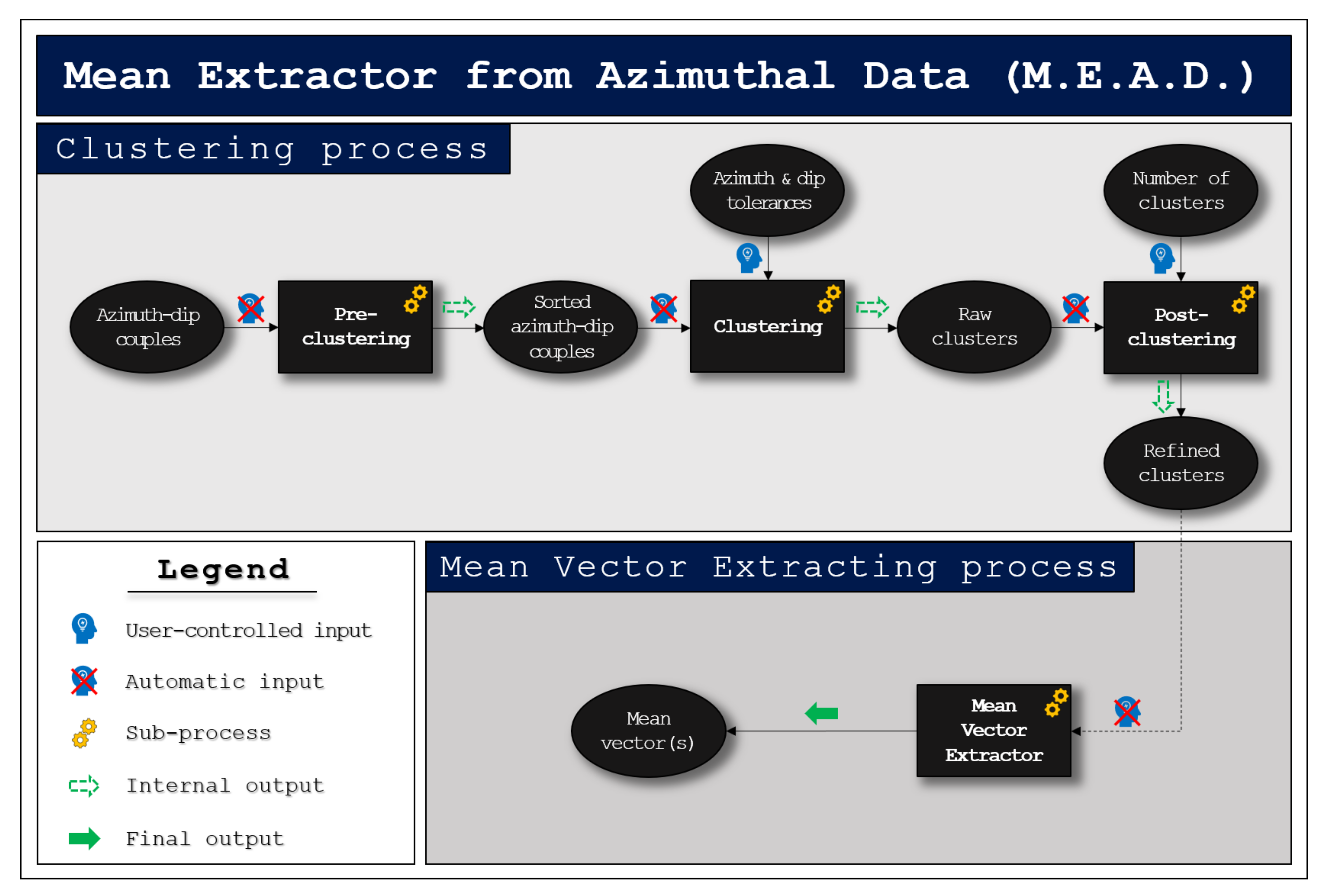
Figure 13) was made by applying a Kamb with linear smoothing method (standard deviation set at 1.5). It shows a reasonably well-defined maximum of subvertical foliations that are steeply dipping towards the SW or NE. A second minor cluster of subvertical foliations also occur dipping toward the N-S. The mean output values for foliations are 311/74 and 316/69 (strike/dip notation) calculated with the K-means and M.E.A.D. + Fisher algorithms (azimuth tolerance = 50%, inclination tolerance = 30%, Fisher confidence = 95%), respectively. At the same site, the stretching lineations (n = 10) are roughly dispersed along the mean plane of the mylonitic foliation, and display subhorizontal to moderate plunges. The Bingham best fit plane of lineations distribution is 320/66 (strike/dip notation).
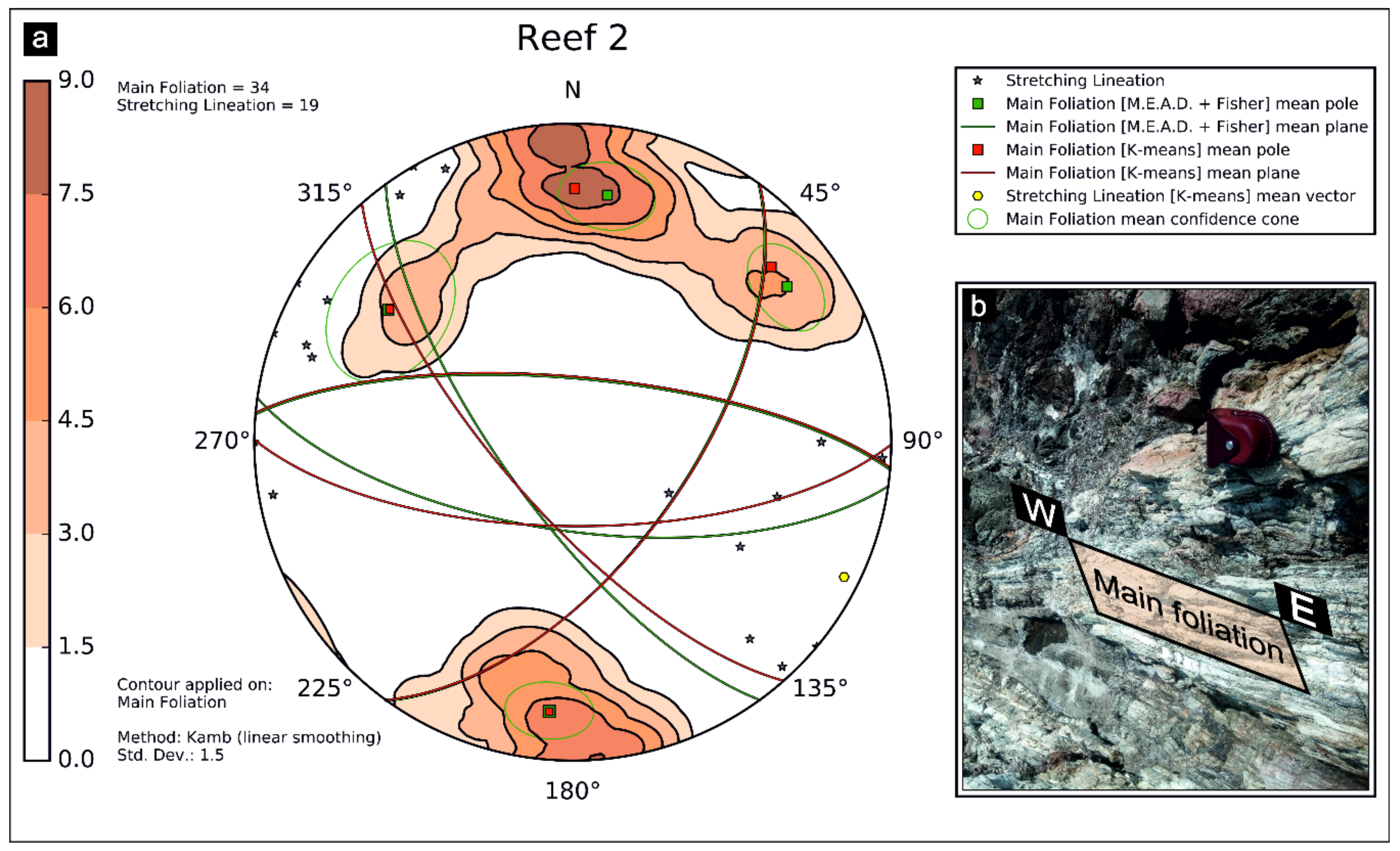
At the second station named ‘Reef 2′, we collected mylonitic foliation (n = 34) as well as stretching lineations (n = 19). Contouring of poles to foliations shows four clusters on the stereoplot (Figure 14). Two clusters are gently dipping towards the N-S, whereas the other two are NE and NW oriented, respectively. The M.E.A.D. + Fisher algorithm (azimuth tolerance = 30%, inclination tolerance = 30%, Fisher confidence = 95%) extracted four size-decreasing ordered clusters (i.e., 098/67; 275/74; 036/61; 144/72) (Figure 14) as shown in the stored related log file available in Table A4 within Appendix B. The mean planes extracted by the K-means algorithm displays similar values (i.e., 090/68; 139/72; 036/60; 275/74), but are randomly sorted and without any indication of predominant clusters. The result of the first algorithm highlighted as the main former clusters display a reasonably good correlation with the previous station, even if rotated by about 35° around a vertical axis. For the stretching lineations, we preferred to apply the K-means algorithm to extract the stretching lineations mean vector (116/05 trend/plunge notation), since the occurrence of supplementary trend values, as already explained in the first case study from Macduff.
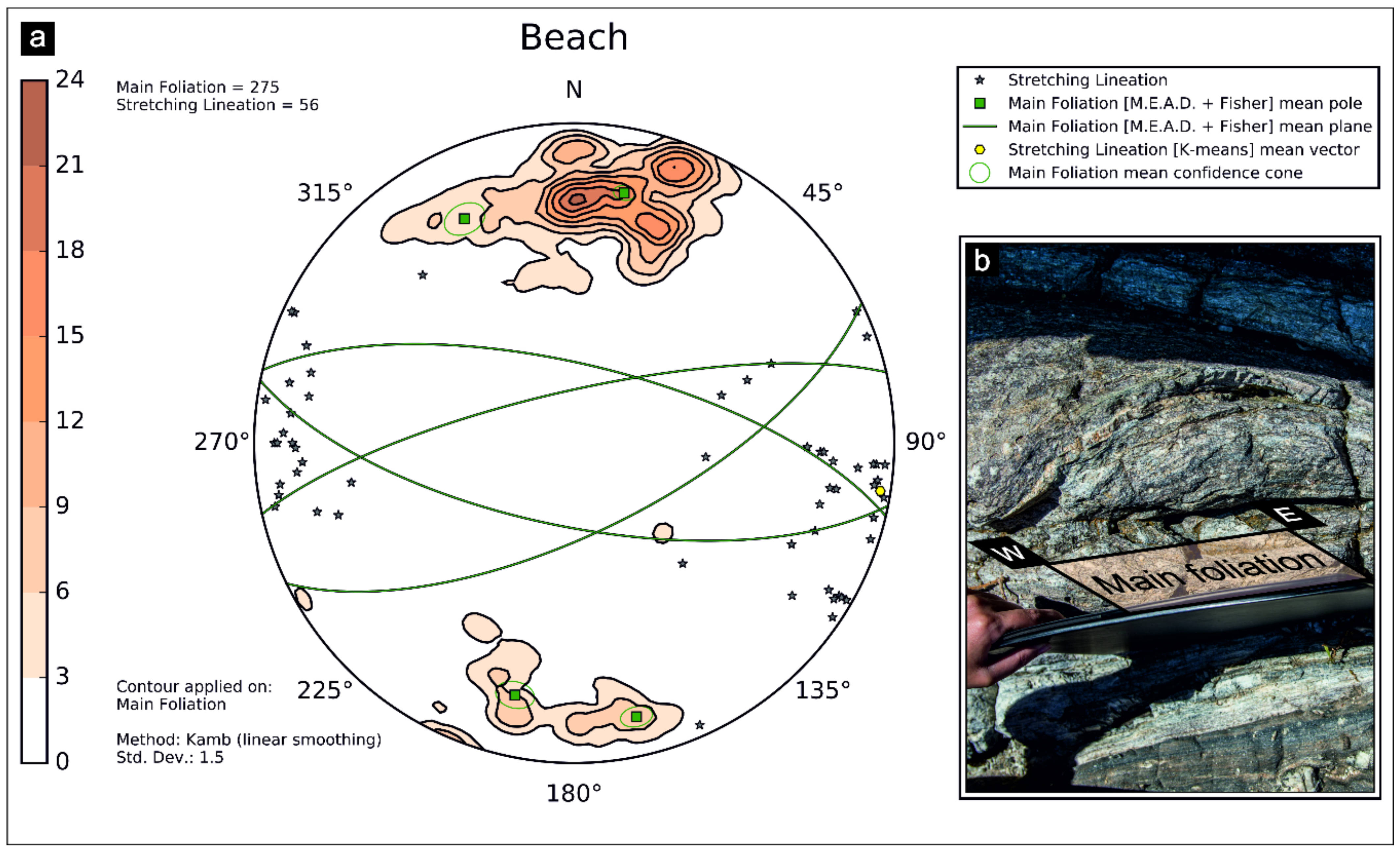
At the third station along the beach, several useful outcrops are well exposed. The 275 available mylonitic foliations depict a main northward cluster followed by a secondary southward one. The application of M.E.A.D. + Fisher algorithm set preliminary with a high number of cluster constraints, highlighted more than eight or nine clusters, with the large number of coalescing data due to the occurrence of highly strained isoclinal folds evolving into sheath folds. Setting the ‘Number of Clusters’ parameter to four, the obtained mean vectors are: 101/69, 283/70, 064/67, 257/77 (strike/dip notation, azimuth tolerance = 20%, inclination tolerance = 20%, Fisher confidence = 95%), which followed the trend of the results of previous structural stations. In this case, we also used a K-means approach for the stretching lineations (n = 56) mean vector extraction. The result is a nearly subhorizontal mean lineation (099/04—trend/plunge notation) (Figure 15), as a consequence of the occurrence of two quite dispersed clusters around E and W directions.
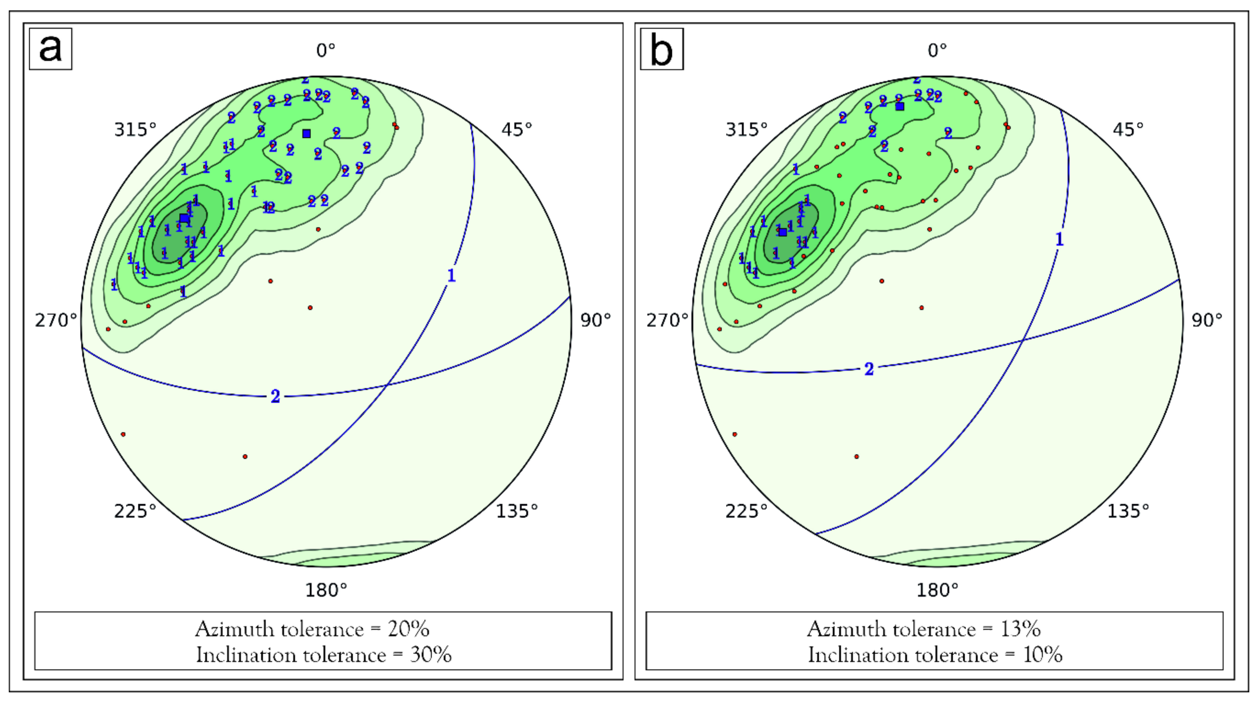
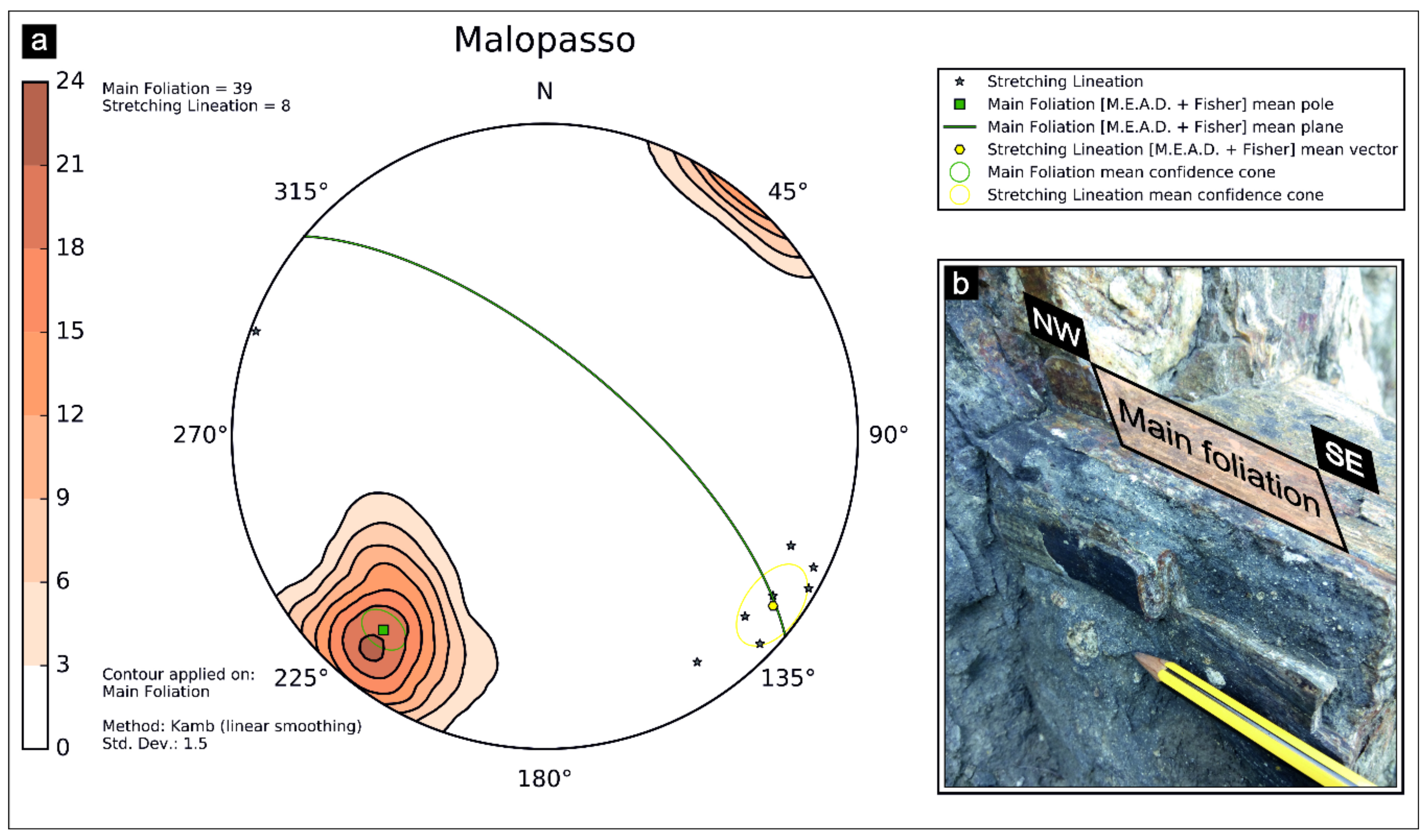
The fourth structural station, located close to the Malopasso locality (Figure 1 and Figure 7), consists of 39 mylonitic foliations and 8 stretching lineations. In this case, all the applied mean extracting algorithms, for both main foliations and stretching lineations, converge. Therefore, we selected the M.E.A.D. + Fisher algorithm to show two confidence cones (Figure 16). The green confidence cone surrounds the pole to mean foliation (310/69—strike/dip notation) with a Fisher angle of 5.28 degrees, while the yellow one is referred to the stretching lineation mean vector (127/10—trend/plunge notation), with Fisher angle of 9,29 degrees (see Table A6 in Appendix B). In both cases, we set the following algorithm-control parameters: azimuth tolerance = 50%, inclination tolerance = 30%, Fisher confidence = 95%.
In general, the orientations of all mesoscopic structures collected at the various localities are quite similar, with only slight differences. In particular, a good association between foliations collected at the first station (Figure 13) and the fourth Malopasso station (Figure 16) has been observed. These stations, which are the northernmost studied localities within the PSZ, have steeply dipping NE-dipping foliations (ca. 70°) with an average NW–SE strike and subhorizontal NW–SE oriented stretching lineations. The other structural stations show a mainly E-W striking foliation that dips either to the N or S (ca. 75°) and is associated with horizontal stretching lineations dispersed toward the E and W.

3.2.2. Microstructural Data Analysis

Two thin sections have been selected for quantitative microstructural analysis in order to create rose diagrams with ASN (see Ortolano et al. [
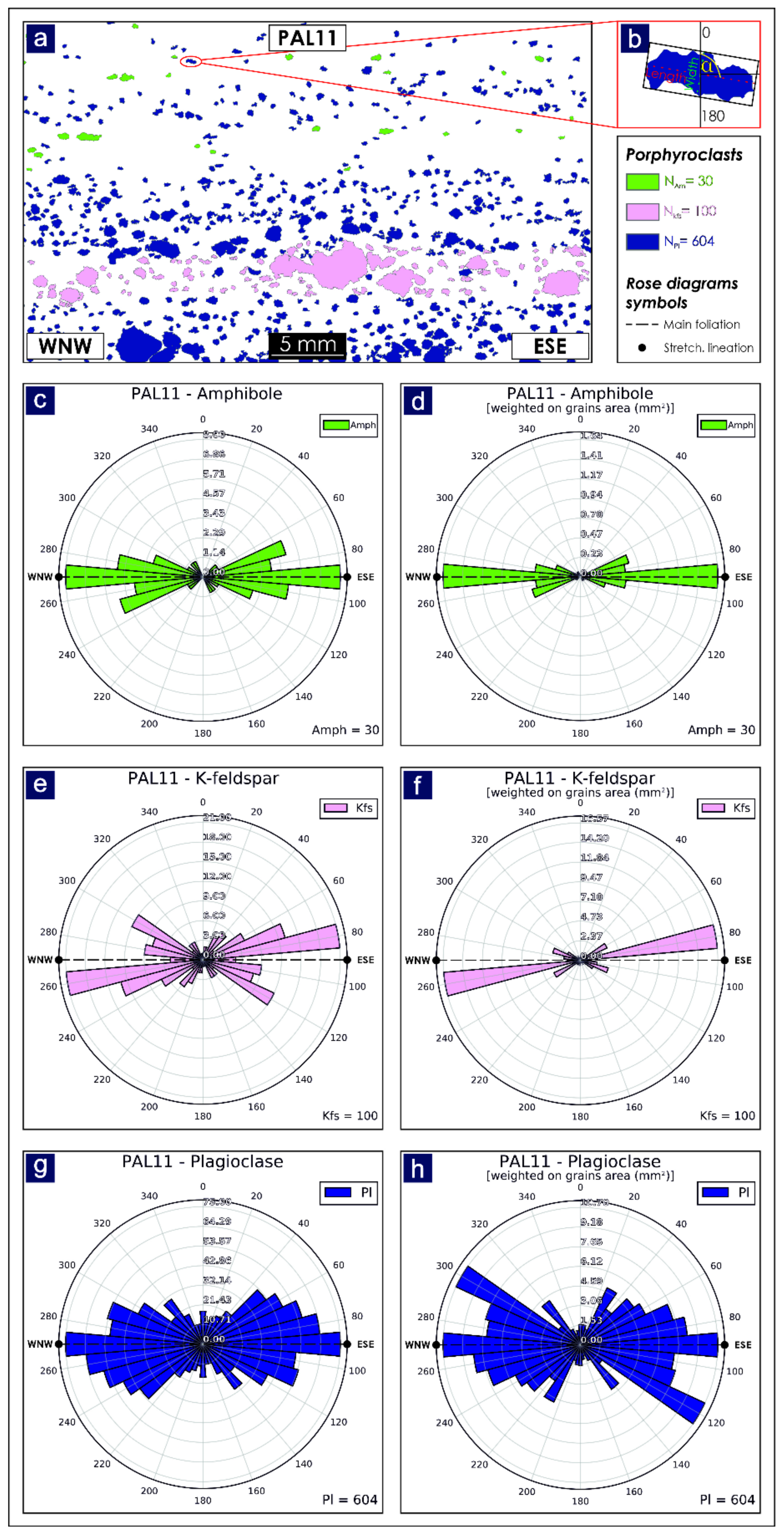
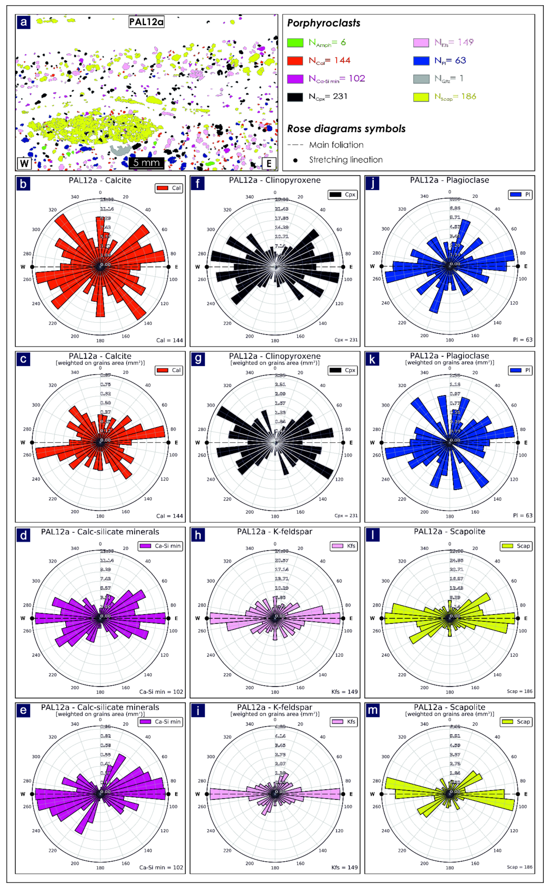
4] for details of microstructure). These rose diagrams depict the preferred orientations of minerals belonging to porphyroclastic domains, where pre-kinematic clasts behave as rigid phases during subsimple shearing plastic deformation. The samples, PAL11 and PAL12a (Figure 12, Figure 17a and Figure 18a), consist of a mylonitic paragneiss from the ‘Malopasso’ station and a mylonitic skarn collected from near the ‘Beach’ station, respectively. The thin section analysis was performed by means of the Min-GSD routine within the Micro-Fabric Analyzer tool [47] which, operating already within the ArcGIS® platform, is suitable as an ‘ASN-friendly’ input feature. The 2D orientation data, obtained via Min-GSD through a stepwise controlled overlaying procedure of X-Ray and Grain-boundary maps of thin sections, permitted storage of microstructural information of minerals in shapefile format [47] (Figure 17a and Figure 18a), and is provided in Table S3 and Table S4 within Supplementary Materials. Specifically, the minimum bounding geometry approach was applied to about 800 clasts per thin section, with the azimuthal values of the preferred orientation of porphyroclasts ranging from 0 to 180 degrees with respect to the normal axis to the main foliation of the sample (Figure 17b). These values can be computed by the ‘Rose Diagrams’ tool while the feature type input parameter can be filled with the mineral name field. Six and twelve rose diagrams have been created, respectively, for PAL11 and PAL12a samples. In both samples, we constructed standard rose diagrams (Figure 17c,e,g, and Figure 18b,d,f,h,j,l), which display directional data and the frequency of minerals, and also weighted rose diagrams (Figure 17b,f,h, and Figure 18c,e,g,i,k,m), which were useful to assign greater or smaller importance to each grain orientation as a function of a specific weighting factor (e.g., their area in mm2). In both cases, we selected the ‘Mirrored behaviour’ option as the azimuthal values only range from 0 to 180 degrees.
For the mylonitic paragneiss (PAL11), a total of 30 amphibole porphyroclasts, 100 K-feldspars and 604 plagioclases were analysed.
The unweighted rose diagram for the amphiboles, which have equivalent spherical diameters [48] (ESD) ranging from 0.25 mm to 0.83 mm, highlights a maximum alignment (i.e., 90°–270°) parallel to the mylonitic foliation, which is oriented in a WNW–ESE direction (Figure 17c). In addition, a weaker alignment with an orientation that deviates by ~20 degrees from the main foliation, can also be recognized. The same results are obtained from the weighted rose diagram (Figure 17d), which does however assign less statistical impact to grains showing an orientation that deviates from the main foliation, due to their small cumulative area.
The unweighted rose diagram for the K-feldspars (0.25 mm < ESD < 3.67 mm) highlights a maximum alignment (i.e., 80°–260°) that deviates by ~10 degrees from the main foliation (Figure 17e), although several families with orientations that vary about the 120°–300° and 40°–220° directions also occur. However, the existence of these families is minimized by the weighted rose diagram (Figure 17f), which shows a clear orientation at 80°–260°, preserved especially by the largest porphyroclasts, where the simple shear component is more pronounced (see Ortolano et al. [4] for details).
Similar to the amphiboles, the unweighted rose diagram for the plagioclases (0.25 mm < ESD < 2.45 mm) highlights a prevalent orientation (i.e., 90°–270°) along the mylonitic foliation (Figure 17g). However, several families show a dispersal in orientation towards N-S and E-W directions with respect to the main foliation, probably linked to the activation of S-C’ planes. This dispersion is highlighted by the weighted rose diagram (Figure 17h), in which the most weighted porphyroclasts show a clear trend along the N-S direction (i.e., 120°–300°).
The mylonitic skarn (PAL12a) allowed us to process a total of 144 calcite clasts, 102 calc-silicate minerals, 231 clinopyroxenes, 149 K-feldspars, 63 plagioclases and 186 scapolite porphyroclasts, with the calculated orientations illustrated in Figure 18.
The unweighted rose diagram for the calcite porphyroclasts (0.18 mm < ESD < 0.50 mm) highlights high dispersion in the orientation data with respect to the mylonitic foliation oriented on average E-W (Figure 18b). Most weighted grains do however show a dominant orientation about E-W (i.e., 80°–260°) as also obtained with the weighted rose diagram (Figure 18c).
The unweighted rose diagram for the calc-silicates (0.18 mm < ESD < 0.79 mm) highlights a lesser dispersion in the orientation data when compared with calcite porphyroclasts, with a high number of grains aligned parallel to the mylonitic foliation (Figure 18d). Nevertheless, by considering the cumulative area of porphyroclasts with the same orientation, as highlighted by the weighted rose diagram (Figure 18e), other families oriented about NE–SW (i.e., 30°–210°) and WNW-ESE (i.e., 110°–290°) orientations can also be recognized.
Similar to the previous mineral phases, the unweighted rose diagram for the clinopyroxenes (0.18 mm < ESD < 1.21 mm) highlights high dispersion in the orientation data with respect to the mylonitic foliation (Figure 18f). Such dispersion is also shown by the weighted rose diagram (Figure 18g), with a dominant ESE–WNW orientation (i.e., 120°–300°) observed.
The unweighted rose diagram for the K-feldspars (0.18 mm < ESD < 1.35 mm) highlights a maximum alignment (i.e., 90°–270°) parallel to the main foliations (Figure 18e). Such alignment is also preserved in the weighted rose diagram (Figure 18i), where fewer families show a ~N-S orientation (i.e., 20°–200°).
Similar to the calcite porphyroclasts, the unweighted rose diagram for the plagioclases (0.18 mm < ESD < 1.03 mm) highlights high dispersion in the orientation data (Figure 18j), with a dominant trend about the E-W (i.e., 80°–260°) and N-S (i.e., 20°–200°) directions. This dispersion is made even more evident by the weighted rose diagram (Figure 18k).
The unweighted rose diagram for the scapolites (0.18 mm < ESD < 7.26 mm) highlights two dominant alignments oriented about the E–W (i.e., 90°–270°) and ENE–WSW (i.e., 50°–230°) directions (Figure 18l), which are further emphasized in the weighted rose diagram (Figure 18m).
Unlike the mylonite paragneiss (PAL11), a greater dispersion in the orientation of the porphyroclasts is observed in the mylonitic skarn (PAL12a) due to the higher contrast in behaviour between weakening (i.e., calcite) and hardening (i.e., porphyroclasts) layers. This leads to a major passive rotation of the PAL12a porphyroclasts during the mylonitic flow due to the high rheology contrast with respect to the calcite weak layers. Differently, PAL11 porphyroclasts, which are surrounded by quartz-rich weak layers (i.e., with a lower rheology contrast with respect to PAL12a), facilitate wing formation, producing greater resistance to the mylonitic flow and, in turn, a clearer evidence of subsimple shear kinematic indicator formation.

4. Discussions

ArcStereoNet is a new Python-toolbox that merges the main ArcGIS® features with the semi-automatic creation of stereoplots, and is compatible with the latest versions of ArcMap® (versions 10.3+).
The reason we chose to use the ESRI ArcGIS® platform, rather than other GIS software, arises from the fact that, starting from the 10.1 version, it is possible to create various personalised Python toolboxes (i.e., that can use several open access Python libraries). These can be linked together with other existing tools (i.e., Model Builder [2,28,29,47]) within a very user-friendly ArcGIS®-like GUI. Furthermore, since the Python version attached to ArcGIS® differs according to ArcGIS® version itself, then the ASN code is able to recognize it and consequently adapt the automatic download and installation routine of the suitable libraries. This extends its compatibility from ArcGIS® 10.3 to the latest distribution (see Supplementary Material—S5).
Even though the use of the open-source library developed by Kington [30] (i.e., mplstereonet) permits the use of most of the ASN applications directly from a Python console, the development of the ASN Python-toolbox opens the possibility of creating lower-hemisphere azimuthal projections and rose diagrams within an ArcGIS® supported GUI for non-Python users. Moreover, ASN allows the user to easily compare several types of analytical statistical methods, including, for the first time, a totally new clustering and mean vector extracting algorithm (Mean Extractor from Azimuthal Data). The M.E.A.D. clustering process takes as input the orientation data, expressed as a list of azimuth-dip couples (i.e., strike-dip for planar features or trend-plunge for linear features), and groups it into a user-defined number of families (i.e., the ‘Number of Clusters’ parameter). The degree of tolerance is driven by two user-controlled percentage values, allowing, in turn, a more incisive analytical choice (see Figure 4). The tool also helps the user in setting the algorithm-control parameters, by providing the possibility to track the behaviour of the M.E.A.D. clustering process (Figure 3d and Figure 5).
ASN joins the classical GIS capabilities of correlating each single projected data point with the corresponding geographical/locality position, thereby merging or subdividing groups of structural stations with a simple procedure. In this view, the ‘Graph to Hyperlink’ tool is used to connect the realised plots with the geographic position of the plotted data, via hyperlink.
Finally, the rose diagrams constructions are applicable, not only for analysis of 2D fault/joint planes orientations, but also for the 2D orientation of microstructural fabric parameters, such as those deriving from grain shape analysis of grain boundary maps in thin sections (e.g., [47]). ASN, however, is potentially capable of working with any type of 2D or 3D oriented data.
The abovementioned specifications drive the ASN-user towards a greater awareness of the average data extrapolation through quick and effective comparisons, by linking the geo-databases manipulation with automatization of various spatially distributed data specific to the GIS environment. In such a way, the user can at any time visualise exactly, within their GIS project, the plotted data together with the corresponding geographical/locality position.
ArcStereoNet follows on the heels of its predecessors developed on the ESRI platform, of which the pioneer is certainly the first tool developed in Avenue [49] for ArcView 3.x by Knox-Robinson and Gardoll [17]. With the development of ArcMap®, other toolbars and add-ins were designed, such as the Export Toolbox [24], written in VBA, that provided methods to export oriented data managed in ArcMap® 8.2 to 3D geoscientific modelling tools (i.e., Editeur Géologique, developed by BRGM, and GOCAD® [50]) and also integrated a spatial averaging routine within ArcMap® itself. These tools are obviously out-dated and no longer compatible with recent versions of ArcGIS® which in the meantime has evolved towards more open data sharing modes and scripting methods.
The most recent tool working within ArcGIS® environment is OATools [25], an add-in for ArcMap® 10.2 and 10.3 versions, written in Visual Basic.NET (VB.NET). This takes advantage of GIS functionalities to carry out the spatial analysis of structural data. Its main features include azimuthal projection of oriented data, extraction of mean vector and fold axes, creation of density distribution diagrams, creation of rose histograms, and mapping of spatial averages.
ArcStereoNet is, therefore, the first entirely Python-coded ArcGIS® tool for the analysis of 3D and 2D oriented datasets. As a result, it smoothly blends with other built-in ArcGIS® toolboxes and its functionalities could be considerably expanded or enhanced thanks to the huge amount of available open access Python libraries. Python-toolboxes are in fact the ESRI suggested approach for creating Python-based tools since ArcGIS® 10.1 version. Moreover, ASN brings in the possibility of choosing between several methods to carry out clustering analysis (for the first time applicable also to rose diagrams) and mean vector extraction, as well as various density distribution functions, thereby providing the user a wide range of statistical analysis techniques to apply to oriented data.

5. Conclusions

ArcStereoNet is the first ArcGIS® Python-toolbox for azimuthal projections useful for 2D and 3D oriented data analysis. It encourages greater user awareness via a stepwise guided control of the different analytical techniques used for 3D and 2D data projections in a GIS environment.
The main features introduced by this new toolbox are:
  • A totally new clustering and mean-vector extracting algorithm used to obtain size-decreasing ordered clusters (i.e., M.E.A.D), and which enables a greater background noise control through tolerance parameters.
  • The capability of analysing both cluster and girdle-like distribution patterns with several algorithms.
  • The capability of contemporaneously running multiple data analysis algorithms to extract statistical parameters.
  • The capability of storing applied algorithm results on automatically compiled log files.
  • The capability of testing several parameter settings at a time via the use of temporary images that do not waste disk memory.

Supplementary Materials

The following are available online at https://0-www-mdpi-com.brum.beds.ac.uk/2220-9964/10/2/50/s1, ArcStereoNet toolbox (S1), Table S2: Palmi meso-structural database, Table S3: PAL11 micro-strucutral database, Table S4: PAL12a micro-strucutral database, User Guide (S5).

Author Contributions

Conceptualization: Gaetano Ortolano, Alberto D’Agostino, Methodology: Alberto D’Agostino, Gaetano Ortolano, Michele Zucali, Roberto Visalli, Software: Alberto D’Agostino, Gaetano Ortolano, Michele Zucali, Roberto Visalli Validation: G. Ian Alsop, Eugenio Fazio, Michele Zucali, Formal Analysis: Gaetano Ortolano, G. Ian Alsop, Michele Zucali, Data resources: Gaetano Ortolano, Rosolino Cirrincione, Mario Pagano, Eugenio Fazio, Roberto Visalli; Data Curation: Alberto D’Agostino, Roberto Visalli, Mario Pagano, Eugenio Fazio, G. Ian Alsop, Writing-Original Draft Preparation: Gaetano Ortolano, Alberto D’Agostino, Roberto Visalli, Eugenio Fazio, Writing-Review & Editing: Michele Zucali, G. Ian Alsop, Rosolino Cirrincione, Figure editing: Alberto D’Agostino, Gaetano Ortolano, Mario Pagano, Roberto Visalli, Supervision: Gaetano Ortolano, Rosolino Cirrincione; Project Administration: Gaetano Ortolano, Rosolino Cirrincione; Funding Acquisition: Gaetano Ortolano, Rosolino Cirrincione. All authors have read and agreed to the published version of the manuscript.

Funding

This research was funded by University of Catania (PIAno di inCEntivi per la RIcerca di Ateneo 2020/2022—Pia.Ce.Ri), Grant Number: 22722132153, within the project: ”Combined geomatic and petromatic applications: The new frontier of geoscience investigations from field- to micro- scale—(GeoPetroMat)”.

Institutional Review Board Statement

Not applicable.

Informed Consent Statement

Not applicable.

Data Availability Statement

The data and the software presented in this study are available online in Supplementary Materials.

Acknowledgments

The authors are grateful to the anonymous reviewers for their helpful suggestions that helped to improve the manuscript.

Conflicts of Interest

The authors declare no conflict of interest.

Appendix A

Within this section, two variants of the Macduff dataset are provided, with the former (Table A1) classifying all data types as generic ‘Fold limb’ and the latter (Table A2) differencing data types between ‘West limb of Anticlines’ and ‘East limb of Anticlines’.
Table A1. Macduff dataset without any data differentiation evidenced by the field investigator (i.e., all data is labelled as generic ‘Fold limb’).
IDAzimuthDip_AngleMethodType
020665RHRFold limb
121225RHRFold limb
221740RHRFold limb
319724RHRFold limb
419220RHRFold limb
521340RHRFold limb
620674RHRFold limb
720568RHRFold limb
819035RHRFold limb
921235RHRFold limb
1020385RHRFold limb
1120552RHRFold limb
1221055RHRFold limb
1320448RHRFold limb
1420670RHRFold limb
1521283RHRFold limb
1621584RHRFold limb
1721077RHRFold limb
1821481RHRFold limb
1920780RHRFold limb
2020581RHRFold limb
2120786RHRFold limb
2220685RHRFold limb
2321463RHRFold limb
243065RHRFold limb
254570RHRFold limb
262775RHRFold limb
273383RHRFold limb
283374RHRFold limb
294070RHRFold limb
301565RHRFold limb
313476RHRFold limb
323275RHRFold limb
333288RHRFold limb
343480RHRFold limb
353580RHRFold limb
363270RHRFold limb
371585RHRFold limb
382472RHRFold limb
392570RHRFold limb
Table A2. Macduff dataset with data differentiation evidenced by the field investigator (i.e., data is split into ‘West limb of Anticlines’ and ‘East limb of Anticlines’).
IDAzimuthDip_AngleMethodType
020665RHRWest limb of Anticlines
121225RHRWest limb of Anticlines
221740RHRWest limb of Anticlines
319724RHRWest limb of Anticlines
419220RHRWest limb of Anticlines
521340RHRWest limb of Anticlines
620674RHRWest limb of Anticlines
720568RHRWest limb of Anticlines
819035RHRWest limb of Anticlines
921235RHRWest limb of Anticlines
1020385RHRWest limb of Anticlines
1120552RHRWest limb of Anticlines
1221055RHRWest limb of Anticlines
1320448RHRWest limb of Anticlines
1420670RHRWest limb of Anticlines
1521283RHREast limb of Anticlines
1621584RHREast limb of Anticlines
1721077RHREast limb of Anticlines
1821481RHREast limb of Anticlines
1920780RHREast limb of Anticlines
2020581RHREast limb of Anticlines
2120786RHREast limb of Anticlines
2220685RHREast limb of Anticlines
2321463RHREast limb of Anticlines
243065RHREast limb of Anticlines
254570RHREast limb of Anticlines
262775RHREast limb of Anticlines
273383RHREast limb of Anticlines
283374RHREast limb of Anticlines
294070RHREast limb of Anticlines
301565RHREast limb of Anticlines
313476RHREast limb of Anticlines
323275RHREast limb of Anticlines
333288RHREast limb of Anticlines
343480RHREast limb of Anticlines
353580RHREast limb of Anticlines
363270RHREast limb of Anticlines
371585RHREast limb of Anticlines
382472RHREast limb of Anticlines
392570RHREast limb of Anticlines

Appendix B

Within this section, four log files, automatically compiled by ASN, are provided. They store results and statistical information of the algorithms applied on Palmi mesostructural data.
Table A3. ‘Reef 1′ station log file. The original .txt file has been converted to table format.
REEF 1
Main Foliation = 112
Stretching Lineation = 10
CONTOUR INFO
Applied on ->Main Foliation
Method ->Kamb (linear smoothing)
St.Dev. ->1.5
STATISTICS
Main Foliation [K-means mean(s)] ->311/74
Main Foliation [M.E.A.D. + Fisher mean(s)] ->316/69
Main Foliation [Fisher Stats]:
- R value (length of the mean vector) ->0.924
- Fisher angle (confidence radius) ->4.62 deg
- K value (dispersion factor) ->13.02
Stretching Lineation [Bingham best fit plane] ->320/66
Note that mean values are expressed as follows:
- strike/dip (planar features)
- trend/plunge (linear features)
Log file automatically compiled by ArcStereoNet
Table A4. ‘Reef 2′ station log file. The original .txt file has been converted to table format.
REEF 2
Main Foliation = 34
Stretching Lineation = 19
CONTOUR INFO
Applied on ->Main Foliation
Method ->Kamb (linear smoothing)
St.Dev. ->1.5
STATISTICS
Main Foliation [K-means mean(s)] ->036/60090/68139/72275/74
Main Foliation [M.E.A.D. + Fisher mean(s)] ->098/67275/74036/61144/72
Main Foliation [Fisher Stats]:
- R value (length of the mean vector) ->0.9410.9660.9630.996
- Fisher angle (confidence radius) ->10.30 deg9.06 deg16.93 deg10.04 deg
- K value (dispersion factor) ->15.8726.3621.38151.70
Stretching Lineation [K-means mean(s)] ->116/05
Note that mean values are expressed as follows:
- strike/dip (planar features)
- trend/plunge (linear features)
Log file automatically compiled by ArcStereoNet
Table A5. ‘Beach’ station log file. The original .txt file has been converted to table format.
BEACH
Main Foliation = 275
Stretching Lineation = 56
CONTOUR INFO
Applied on ->Main Foliation
Method ->Kamb (linear smoothing)
St.Dev. ->1.5
STATISTICS
Main Foliation [M.E.A.D. + Fisher mean(s)] ->101/69283/70064/67257/77
Main Foliation [Fisher Stats]:
- R value (length of the mean vector) ->0.9670.9690.9690.994
- Fisher angle (confidence radius) ->2.22 deg4.09 deg4.52 deg3.22 deg
- K value (dispersion factor) ->30.1631.5531.55153.40
Stretching Lineation [K-means mean(s)] ->099/04
Note that mean values are expressed as follows:
- strike/dip (planar features)
- trend/plunge (linear features)
Log file automatically compiled by ArcStereoNet
Table A6. ‘Malopasso’ station log file. The original .txt file has been converted to table format.
MALOPASSO
Main Foliation = 39
Stretching Lineation = 8
CONTOUR INFO
Applied on ->Main Foliation
Method ->Kamb (linear smoothing)
St.Dev. ->1.5
STATISTICS
Main Foliation [M.E.A.D. + Fisher mean(s)] ->310/69
Main Foliation [Fisher Stats]:
- R value (length of the mean vector) ->0.957
- Fisher angle (confidence radius) ->5.28 deg
- K value (dispersion factor) ->22.69
Stretching Lineation [M.E.A.D. + Fisher mean(s)] ->127/10
Stretching Lineation [Fisher Stats]:
- R value (length of the mean vector) ->0.980
- Fisher angle (confidence radius) ->9.29 deg
- K value (dispersion factor) ->43.19
Note that mean values are expressed as follows:
- strike/dip (planar features)
- trend/plunge (linear features)
Log file automatically compiled by ArcStereoNet

References

  1. Ortolano, G.; Visalli, R.; Cirrincione, R.; Rebay, G. PT-path reconstruction via unraveling of peculiar zoning pattern in atoll shaped garnets via image assisted analysis: An example from the Santa Lucia del Mela garnet micaschists (northeastern Sicily-Italy). Period. Miner. 2014, 83, 257–297. [Google Scholar] [CrossRef]
  2. Ortolano, G.; Zappalà, L.; Mazzoleni, P. X-Ray Map Analyser: A new ArcGIS® based tool for the quantitative statistical data handling of X-ray maps (Geo- and material-science applications). Comput. Geosci. 2014, 72, 49–64. [Google Scholar] [CrossRef]
  3. Ortolano, G.; Cirrincione, R.; Pezzino, A.; Tripodi, V.; Zappala, L. Petro-structural geology of the Eastern Aspromonte Massif crystalline basement (southern Italy-Calabria): An example of interoperable geo-data management from thin section—To field scale. J. Maps 2015, 11, 181–200. [Google Scholar] [CrossRef] [Green Version]
  4. Ortolano, G.; Fazio, E.; Visalli, R.; Alsop, G.I.; Pagano, M.; Cirrincione, R. Quantitative microstructural analysis of mylonites formed during Alpine tectonics in the western Mediterranean realm. J. Struct. Geol. 2020, 131, 103956. [Google Scholar] [CrossRef]
  5. Ortolano, G.; Visalli, R.; Fazio, E.; Fiannacca, P.; Godard, G.; Pezzino, A.; Punturo, R.; Sacco, V.; Cirrincione, R. Tectono-metamorphic evolution of the Calabria continental lower crust: The case of the Sila Piccola Massif. Int. J. Earth Sci. 2020, 109, 1295–1319. [Google Scholar] [CrossRef]
  6. Belfiore, C.M.; Fichera, G.V.; Ortolano, G.; Pezzino, A.; Visalli, R.; Zappalà, L. Image processing of the pozzolanic reactions in Roman mortars via X-Ray Map Analyser. Microchem. J. 2016, 125, 242–253. [Google Scholar] [CrossRef]
  7. Fazio, E.; Ortolano, G.; Visalli, R.; Alsop, I.; Cirrincione, R.; Pezzino, A. Strain localization and sheath fold development during progressive deformation in a ductile shear zone: A case study of macro-to micro-scale structures from the Aspromonte Massif, Calabria. Ital. J. Geosci. 2018, 137, 208–218. [Google Scholar] [CrossRef]
  8. Fazio, E.; Ortolano, G.; Visalli, R.; Cirrincione, R.; Kern, H.; Mengel, K.; Pezzino, A.; Punturo, R. Strain rates of the syn-tectonic Symvolon pluton (Southern Rhodope Core Complex, Greece): An integrated approach combining quartz paleopiezometry, flow laws and PT pseudosections. Ital. J. Geosci. 2018, 137, 219–237. [Google Scholar] [CrossRef]
  9. Fazio, E.; Punturo, R.; Cirrincione, R.; Kern, H.; Pezzino, A.; Wenk, H.-R.; Goswami, S.; Mamtani, M.A. Quartz preferred orientation in naturally deformed mylonitic rocks (Montalto shear zone–Italy): A comparison of results by different techniques, their advantages and limitations. Int. J. Earth Sci. 2017, 106, 2259–2278. [Google Scholar] [CrossRef]
  10. Fazio, E.; Punturo, R.; Cirrincione, R. Quartz c-axis texture mapping of mylonitic metapelite with rod structures (Calabria, southern Italy): Clues for hidden shear flow direction. J. Geol. Soc. India 2010, 75, 171–182. [Google Scholar] [CrossRef]
  11. Turner, F.J.; Weiss, L.E. Structural Analysis of Metamorphic Tectonites; McGraw-Hill: New York, NY, USA, 1963; ISBN 978-0-07-065574-4. [Google Scholar]
  12. Phillips, F.C. The Use of Stereographic Projection in Structural Geology, 3rd ed.; Edward Arnold: London, UK, 1971; ISBN 978-0-7131-2342-5. [Google Scholar]
  13. Park, R.G. Foundations of Structural Geology, 3rd ed.; Routledge: London, UK, 2013; ISBN 978-1-136-78435-4. [Google Scholar]
  14. Snyder, J.P. Map Projections—A Working Manual; US Geological Survey Professional Paper 1395; US Government Printing Office: Washington, DC, USA, 1987; ISBN 978-1-78266-222-8.
  15. Grafarend, E.W.; You, R.-J.; Syffus, R. Map Projections; Springer: Berlin/Heidelberg, Germany, 2014; ISBN 978-3-642-36493-8. [Google Scholar]
  16. Hobbs, B.E.; Means, W.D.; Williams, P.F. An Outline of Structural Geology; Wiley: New York, NY, USA, 1985; ISBN 978-0-471-40157-5. [Google Scholar]
  17. Knox-Robinson, C.M.; Gardoll, S.J. GIS-stereoplot: An interactive stereonet plotting module for ArcView 3.0 geographic information system. Comput. Geosci. 1998, 24, 243–250. [Google Scholar] [CrossRef]
  18. Allmendinger, R. Stereonet 11 | Rick Allmendinger’s Stuff. Available online: http://www.geo.cornell.edu/geology/faculty/RWA/programs/stereonet.html (accessed on 25 November 2020).
  19. Vollmer, F.W. C program for automatic contouring of spherical orientation data using a modified Kamb method. Comput. Geosci. 1995, 21, 31–49. [Google Scholar] [CrossRef]
  20. Vollmer, F.W. An application of eigenvalue methods to structural domain analysis. Geol. Soc. Am. Bull. 1990, 102, 786–791. [Google Scholar] [CrossRef]
  21. Vollmer, F.W. Orient 3: A new integrated software program for orientation data analysis, kinematic analysis, spherical projections, and Schmidt plots. In Proceedings of the Geological Society of America Abstracts with Programs, Baltimore, MD, USA, 25–28 October 2015; Volume 47, p. 49. [Google Scholar]
  22. Alberti, M.; Laloux, M.; Zanieri, M. Tools for structural geology analysis in QGIS. Rendiconti. Online Soc. Geol. Ital. 2016, 39, 55–59. [Google Scholar] [CrossRef]
  23. Thiele, S.T.; Grose, L.; Samsu, A.; Micklethwaite, S.; Vollgger, S.A.; Cruden, A.R. Rapid, semi-automatic fracture and contact mapping for point clouds, images and geophysical data. Solid Earth 2017, 8, 1241–1253. [Google Scholar] [CrossRef] [Green Version]
  24. Maxelon, M. Some Tools for Three-Dimensional Modelling in Structural Geology and Tectonics; ETH: Zurich, Switzerland, 2004. [Google Scholar]
  25. Kociánová, L.; Melichar, R. OATools: An ArcMap add-in for the orientation analysis of geological structures. Comput. Geosci. 2016, 87, 67–75. [Google Scholar] [CrossRef]
  26. Fazio, E.; Ortolano, G.; Cirrincione, R. Eye-type folds at the Palmi shear zone (Calabria, Italy). Int. J. Earth Sci. 2017, 106, 2039–2040. [Google Scholar] [CrossRef]
  27. Li, Y.; Onasch, C.M.; Guo, Y. GIS-based detection of grain boundaries. J. Struct. Geol. 2008, 30, 431–443. [Google Scholar] [CrossRef]
  28. Ortolano, G.; Visalli, R.; Godard, G.; Cirrincione, R. Quantitative X-ray Map Analyser (Q-XRMA): A new GIS-based statistical approach to Mineral Image Analysis. Comput. Geosci. 2018, 115, 56–65. [Google Scholar] [CrossRef]
  29. Fiannacca, P.; Ortolano, G.; Pagano, M.; Visalli, R.; Cirrincione, R.; Zappalà, L. IG-Mapper: A new ArcGIS® toolbox for the geostatistics-based automated geochemical mapping of igneous rocks. Chem. Geol. 2017, 470, 75–92. [Google Scholar] [CrossRef]
  30. Kington, J. Joferkington/Mplstereonet. Available online: https://github.com/joferkington/mplstereonet (accessed on 25 November 2020).
  31. Hunter, J.D. Matplotlib: A 2D Graphics Environment. Comput. Sci. Eng. 2007, 9, 90–95. [Google Scholar] [CrossRef]
  32. Oliphant, T.E. A Guide to NumPy, 2nd ed.; CreateSpace Independent Publishing Platform: North Charleston, SC, USA, 2015; ISBN 1-5173-0007-X. [Google Scholar]
  33. Kamb, W.B. Ice petrofabric observations from Blue Glacier, Washington, in relation to theory and experiment. J. Geophys. Res. 1959, 64, 1891–1909. [Google Scholar] [CrossRef]
  34. Fisher, N.I.; Lewis, T.; Embleton, B.J.J. Statistical Analysis of Spherical Data; Cambridge University Press: Cambridge, UK, 1993; ISBN 978-0-521-45699-9. [Google Scholar]
  35. Kington, J. Mplstereonet Package—Mplstereonet 0.6-dev Documentation. Available online: https://mplstereonet.readthedocs.io/en/latest/mplstereonet.html (accessed on 25 November 2020).
  36. MacQueen, J. Some Methods for Classification and Analysis of Multivariate Observations. In Proceedings of the Fifth Berkeley Symposium on Mathematical Statistics and Probability, Oakland, CA, USA, 21 June–18 July 1967; University of California Press: Berkeley, CA, USA, 1967; Volume 1, pp. 281–297. [Google Scholar]
  37. Bingham, C. An Antipodally Symmetric Distribution on the Sphere. Ann. Stat. 1974, 2, 1201–1225. [Google Scholar] [CrossRef]
  38. Trewin, N.H. Macduff, Dalradian Turbidite Fan and Glacial Deposits. In Excursion Guide to the Geology of the Aberdeen Area; Scottish Academic Press: Edinburgh, UK, 1987; pp. 79–88. [Google Scholar]
  39. Chew, D.M.; Strachan, R.A. The Laurentian Caledonides of Scotland and Ireland. Geol. Soc. Lond. Spec. Publ. 2014, 390, 45–91. [Google Scholar] [CrossRef] [Green Version]
  40. Strachan, R.A. The Grampian Orogeny: Mid-Ordovician Arc–Continent Collision along the Laurentian Margin of Iapetus. In Geological History of Britain and Ireland; Blackwell Publishing, Ltd.: Hoboken, NJ, USA, 2012; pp. 91–109. ISBN 978-1-118-27406-4. [Google Scholar]
  41. Hudson, N.F.C.; Johnson, T.E. Macduff to Whitehills—Buchan type regional metamorphic zones. In Excursion guide to the Geology of the Aberdeen Area; Scottish Academic Press: Edinburgh, UK, 1987; pp. 89–98. [Google Scholar]
  42. Prosser, G.; Caggianelli, A.; Rottura, A. Strain localisation driven by marble layers: The Palmi shear zone (Calabria-Peloritani terrane, Southern Italy). GeoActa 2003, 2, 155–166. [Google Scholar]
  43. Cirrincione, R.; Fazio, E.; Fiannacca, P.; Ortolano, G.; Pezzino, A.; Punturo, R. The Calabria-Peloritani Orogen, a composite terrane in Central Mediterranean; Its overall architecture and geodynamic significance for a pre-Alpine scenario around the Tethyan basin. Period. Miner. 2015, 84, 701–749. [Google Scholar] [CrossRef]
  44. Ortolano, G.; Cirrincione, R.; Pezzino, A.; Puliatti, G. Geo-Petro-Structural study of the Palmi shear zone: Kinematic and rheological implications. Rend. Online Soc. Geol. Ital. 2013, 29, 126–129. [Google Scholar]
  45. Ortolano, G.; Cirrincione, R.; Pezzino, A. P-T evolution of Alpine metamorphism in the southern Aspromonte Massif (Calabria-Italy). Schweiz. Mineral. Petrogr. Mitt. 2005, 85, 31–56. [Google Scholar]
  46. Angì, G.; Cirrincione, R.; Fazio, E.; Fiannacca, P.; Ortolano, G.; Pezzino, A. Metamorphic evolution of preserved Hercynian crustal section in the Serre Massif (Calabria-Peloritani Orogen, southern Italy). Lithos 2010, 115, 237–262. [Google Scholar] [CrossRef]
  47. Visalli, R.; Ortolano, G.; Godard, G.; Cirrincione, R. Micro-Fabric Analyzer (MFA): A new semiautomated ArcGIS-based edge detector for quantitative microstructural analysis of rock thin-sections. ISPRS Int. J. Geo-Inf. 2021, 10, 51. [Google Scholar] [CrossRef]
  48. Jennings, B.R.; Parslow, K. Particle size measurement: The equivalent spherical diameter. Proc. Math. Phys. Eng. Sci. 1988, 419, 137–149. [Google Scholar] [CrossRef]
  49. Razavi, A.H.; Warwick, V. ArcView GIS/Avenue Programmer’s Reference: Class Hierarchy Quick Reference and 100+ Scripts, 3rd ed.; OnWord Press: Albany, NY, USA, 2000; ISBN 978-1-56690-170-3. [Google Scholar]
  50. Mallet, J.L. GOCAD: A Computer Aided Design Program for Geological Applications. In Three-Dimensional Modeling with Geoscientific Information Systems; Turner, A.K., Ed.; Springer: Dordrecht, The Netherlands, 1992; pp. 123–141. ISBN 978-94-010-5128-6. [Google Scholar]
Figure 1. Example of ArcMap® (version 10.6.1) equipped with ArcStereoNet. After creating a shapefile storing oriented data (a) and selecting the records stored inside its attribute table (b), the user can open the ArcStereoNet toolbox (c) from the ArcToolbox window and choose the preferred tool.
Ijgi 10 00050 g001
Figure 2. ‘Stereoplots’ tool layout. Green dots indicate required parameters. (a) Oriented dataset input; requires a shapefile (point, line, and polygon features types are supported). (b) Azimuth, Dip Angle, Method, and Type fields inputs, selectable through the drop-down menus. (c) Plotting data Value Table; for each added feature type the user can specify the plotting colour, pole, or vector symbol and size, cyclographic trace style, and width. (d) Output image settings; the stereoplot can be saved as a temporary file by unchecking the ‘Store Image Output’ option, otherwise an output file path can be selected. (e) ‘Contour & Statistics’ submenu; see Figure 3 for details. (f) Plot customisation submenu; enables the look of stereoplot to be customised. (g) Plotting options submenu; the stereonet type can be chosen (equal-area or equal-angle) and the ‘Write Log File’ option can be checked to prompt the tool to compile a text file storing statistical information concerning the plotted data.
Ijgi 10 00050 g002
Figure 3. Expanded ‘Contour & Statistics’ submenu of ‘Stereoplots’ tool. (a) ‘Apply Contour’ Value Table; the user can choose the preferred contour density function under the ‘Method’ column, and set other parameters such as standard deviation, style, colour, and transparency. (b) Show a colour bar referred to the applied contour. (c) ‘Extract Mean Vectors’ Value Table; the algorithm-control parameters are ‘Algorithm’, to choose the preferred algorithm, ‘Number of Clusters’, Azimuth and Inclination tolerances and ‘Fisher confidence’. The other parameters gather settings for graphic appearance. (d) Track Mean Extractor from Azimuthal Data (M.E.A.D.) clustering behaviour option will only apply on clusters extracted by mean of the M.E.A.D. clustering process (see “‘Stereoplots’ tool algorithms” subparagraph for details).
Ijgi 10 00050 g003
Figure 4. Mean Extractor from Azimuthal Data (M.E.A.D.) algorithm flow chart. Ovals indicate input/output objects, squares indicate algorithm subprocesses. The azimuth-dip couples are first sorted by most frequent azimuth value (pre-clustering); then the clustering subprocess is applied, taking care of the user-controlled tolerance parameters. The raw output is then refined in a post-clustering phase and the required number of clusters is returned. Finally, these are fed into the mean vector extracting process that outputs the final result, consisting of one or more mean vectors.
Ijgi 10 00050 g004
Figure 5. Influence of azimuth and inclination tolerance parameters on the M.E.A.D. clustering process, highlighted with ‘Track M.E.A.D. behaviour’ option (Figure 3d). (a) Two-clusters model with an azimuth tolerance of 20% and an inclination tolerance of 30%. Almost all plotted data is grouped into two different clusters (1 and 2). (b) Two-clusters model with an azimuth tolerance of 13% and an inclination tolerance of 10%. Extracted clusters tend to be less dispersed and, consequently, much more data is evaluated as spurious (i.e., not gathered within any cluster).
Ijgi 10 00050 g005
Figure 6. ‘Rose Diagrams’ tool layout. Green dots indicate required parameters. (a) Oriented dataset input; requires a shapefile (point, line, and polygon features types are supported). (b) Azimuth and Type fields inputs, selectable through the drop-down menus. (c) Plotting data Value Table; for each added feature type, the user can specify the bar colour and whether to show the mean vectors or not, with a determined number of clusters and azimuth tolerance. (d) Output image settings; the rose diagram can be saved as a temporary file by unchecking the ‘Store Image Output’ option, otherwise an output file path can be selected. (e) Plot customisation submenu; rose diagram look can be here customised. (f) Plotting options submenu; ‘Mirrored behaviour’ option allows to prompt for a specular rose diagram, ‘Weighted Rose Diagram’ option allows the user to weight data (a weight field must be provided). The ‘Write Log File’ option can be checked to prompt the tool to compile a text file storing statistical information concerning the plotted data.
Ijgi 10 00050 g006
Figure 7. Graph To Hyperlink tool. (a) Tool layout; one or multiple raster images are required as input. Such images are meant to be stereoplots or rose diagrams realised by the ASN related tools. An output feature class is also required; here, the spatial information and the hyperlinks to each image is stored. (b) Example of Graph To Hyperlink result. Green circles indicate four different sampling stations; the corresponding plots pop out from each of them.
Ijgi 10 00050 g007
Figure 8. Field photograph of a NNE-trending upright synform that folds bedding (highlighted in yellow) and develops a broadly axial-planar cleavage (in green). (Macduff area: UK Grid: NJ7190 6465).
Ijgi 10 00050 g008
Figure 9. Application of ArcStereoNet algorithms with default control parameters for the extraction of mean vectors from the Macduff area dataset, treated as a single feature type. (a) ASN graphic result; (b) portion of Macduff dataset attribute table, with all records sharing the same feature type (i.e., “Fold limb”); (c) ASN log file showing algorithm statistics and results; and (d) “Extract Mean Vector” Value Table showing the algorithm settings.
Ijgi 10 00050 g009
Figure 10. Application of ArcStereoNet algorithms with customised control parameters for the extraction of mean vectors from the Macduff area dataset, treated as a single feature type. (a) ASN graphic result; (b) portion of Macduff dataset attribute table, with all records sharing the same feature type (i.e., ‘Fold limb’); (c) ASN log file showing algorithm statistics and results; and (d) ‘Extract Mean Vector’ Value Table showing the algorithm settings.
Ijgi 10 00050 g010
Figure 11. Application of ArcStereoNet algorithms with customised control parameters for the extraction of mean vectors from the Macduff area dataset, grouped in two different feature types. (a) ASN graphic result; (b) portion of Macduff dataset attribute table, with records displaying two different feature types (i.e., ‘East limb of Anticlines’ and ‘West limb of Anticlines’); (c) ASN log file showing algorithm statistics and results; and (d) ‘Extract Mean Vector’ Value Table showing the algorithm settings.
Ijgi 10 00050 g011
Figure 12. Geological background of the Palmi Shear Zone: (a) Geological map of the Calabrian metamorphic complexes (after Angì et al. [46]); (b) Geological Map of the case study area of the Palmi Shear zone with trends of the main foliations and average stretching lineations, (white circles represent location of each structural station, while red circles represent sample locations).
Ijgi 10 00050 g012
Figure 13. ‘Reef 1′ station: (a) equal-area azimuthal projection and statistical analysis of main foliations and stretching lineations data and (b) field example of isoclinally folded foliation in mylonites (tonalites interlayered with paragneisses). The ASN log file is provided in Appendix B (Table A3).
Ijgi 10 00050 g013
Figure 14. ‘Reef 2′ station: (a) equal-area azimuthal projection and statistical analysis of main foliations and stretching lineation data and (b) field example of mylonitic foliation subparallel to fold axial surface in tonalites. The ASN log file is provided in Appendix B (Table A4).
Ijgi 10 00050 g014
Figure 15. ‘Beach’ station: (a) equal-area azimuthal projection and statistical analysis of main foliations and stretching lineation data and (b) field example of W–E oriented mylonitic foliation developed in tonalites interlayered with paragneisses. The ASN log file is provided in Appendix B (Table A5).
Ijgi 10 00050 g015
Figure 16. ‘Malopasso’ station: (a) equal-area azimuthal projection and statistical analysis of main foliations and stretching lineation data and (b) field example of tight isoclinal folds and smaller sheath folds developed in calc-silicates and skarns. The ASN log file is provided in Appendix B (Table A6).
Ijgi 10 00050 g016
Figure 17. Application of ‘Rose Diagrams’ tool to PAL11 microstructural data. (a) Porphyroclast grain boundary detection map obtained via Min-GSD routine [4]; (b) scheme of the minimum bounding geometry data extraction for each single clast, where α represents the angle between the normal to the main foliation in thin section with the major axis of the bounding box; (c,e,g) unweighted rose diagrams; (d,f,h) weighted rose diagrams based on grains cumulative area (in mm2).
Ijgi 10 00050 g017
Figure 18. Application of ‘Rose Diagrams’ tool to PAL12a microstructural data. (a) Porphyroclast grain boundary detection map obtained via Min-GSD routine [4]; (b,d,f,h,j,l) unweighted rose diagrams; (c,e,g,i,k,m) weighted rose diagrams based on grains cumulative area (in mm2).
Ijgi 10 00050 g018
Table 1. Influences of user-controlled parameters on ArcStereoNet (ASN) algorithms. An ‘X’ symbol means that the parameter (row) has an effect on the algorithm (column).
M.E.A.D. + FisherM.E.A.D.K-MeansBingham
Number of ClustersXXX-
M.E.A.D. Azimuth toleranceXX--
M.E.A.D. Inclination toleranceXX--
Fisher ConfidenceX---
Publisher’s Note: MDPI stays neutral with regard to jurisdictional claims in published maps and institutional affiliations.

