
Assessment of Neotectonic Landscape Deformation in Evia Island, Greece, Using GIS-Based Multi-Criteria Analysis

 ,
,  ,
,  ,
, 
Abstract
:1. Introduction
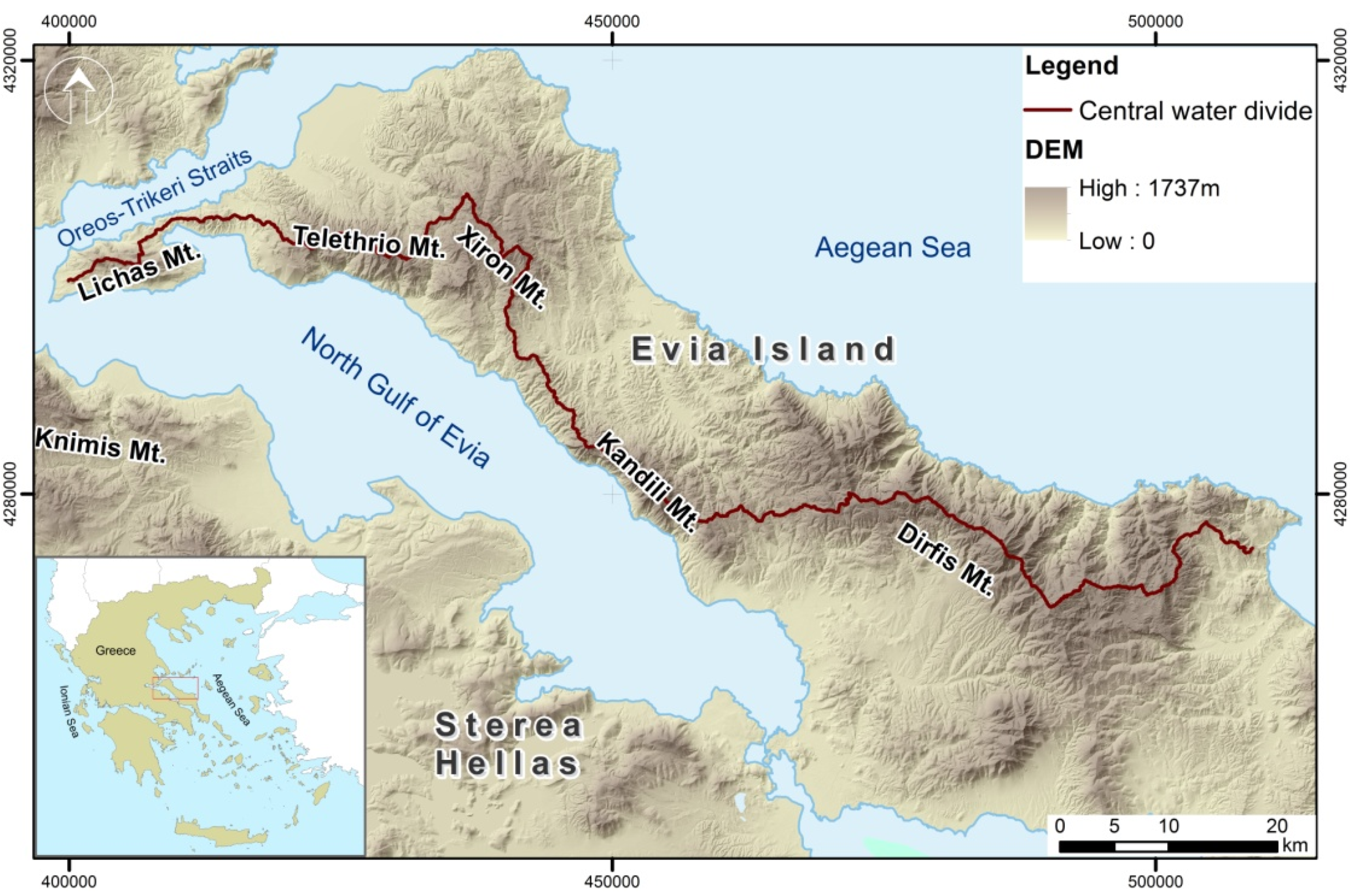
2. Study Area
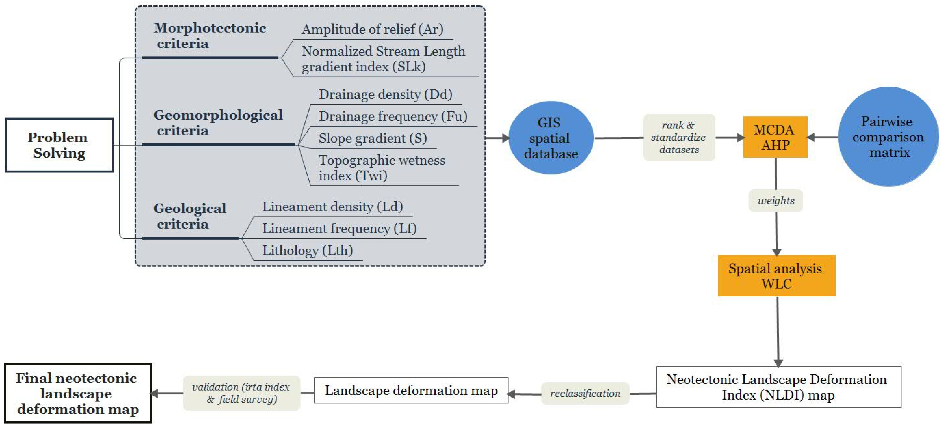
3. Materials and Methods
3.1. Geodatabase
3.2. Multi-Criteria Decision Analysis (MCDA)
Criteria Used
3.3. Analytic Hierarchy Process (AHP)
3.4. Weighted Linear Combination (WLC)
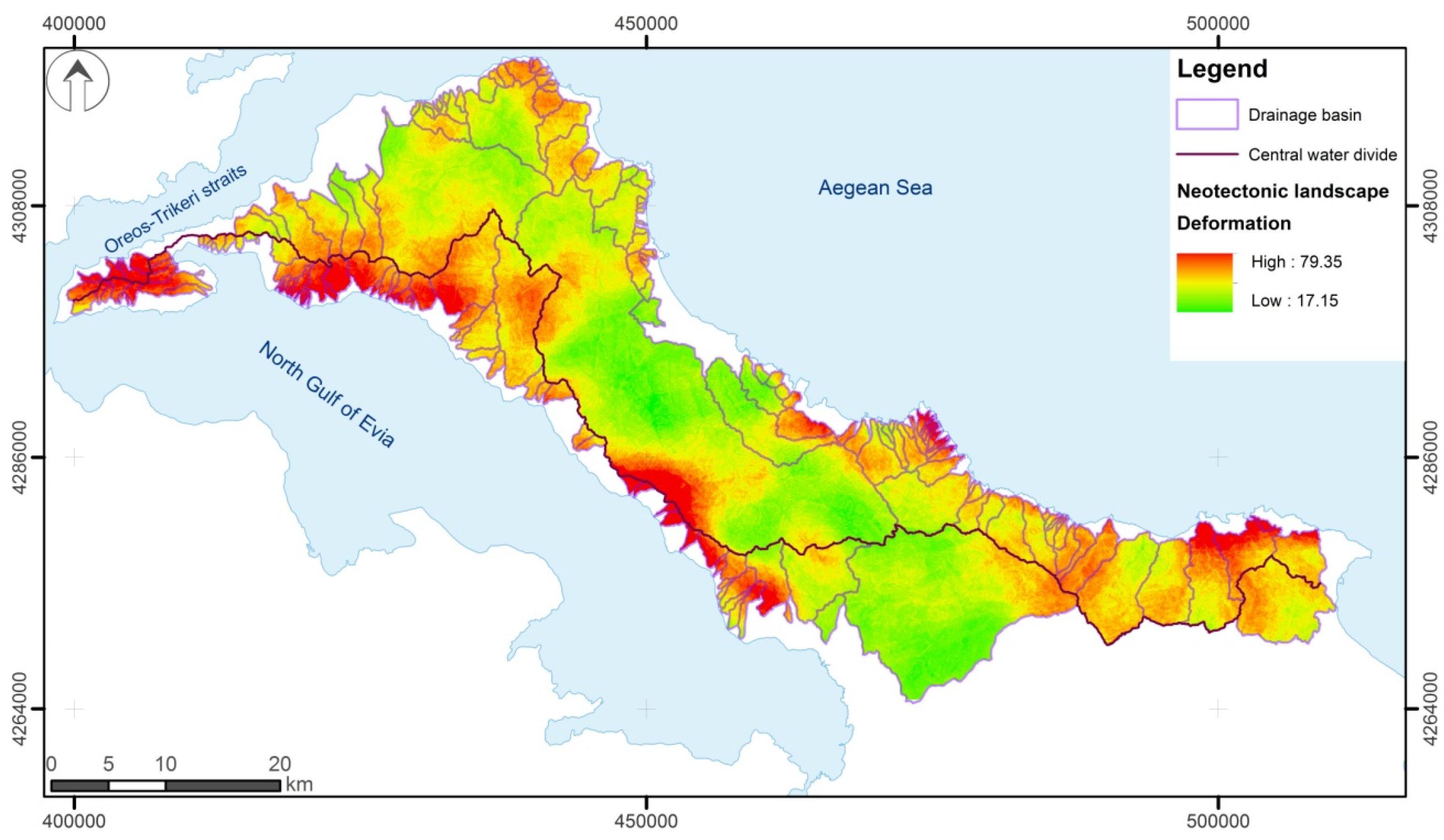
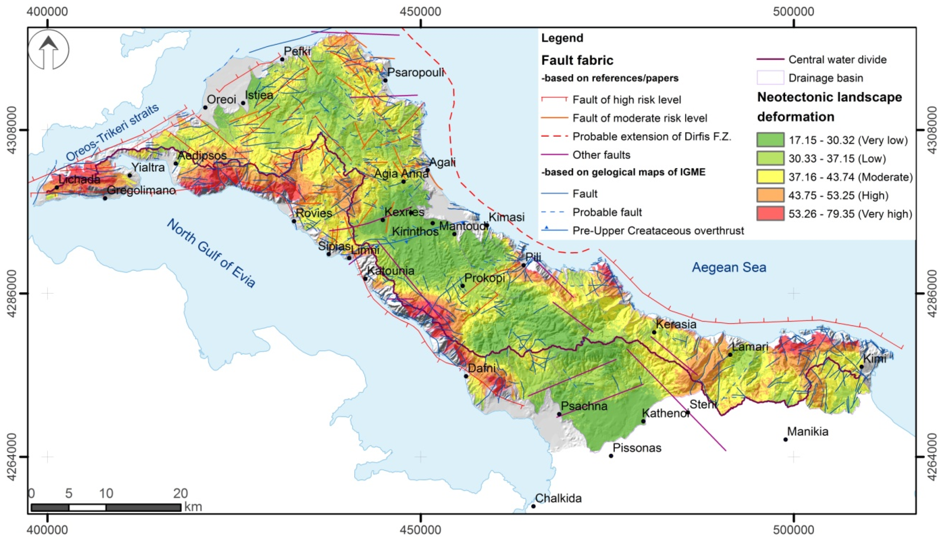
4. Results
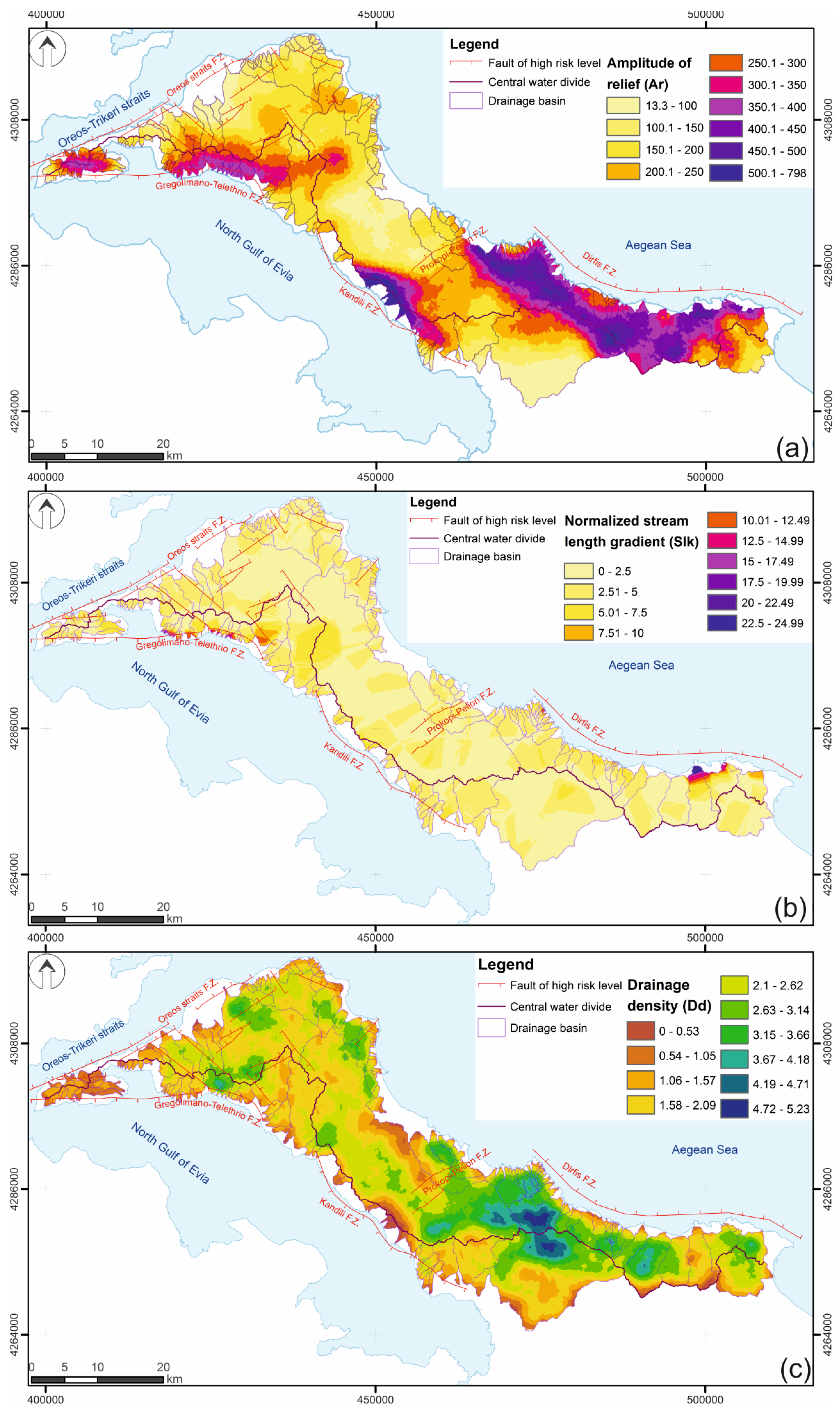
4.1. Conditioning Factors
4.2. Multi-Criteria Decision Analysis
- Very low (17.15–30.32)
- Low (30.33–37.15)
- Moderate (37.16–43.74)
- High (43.75–53.25)
- Very high (53.26–79.35)
5. Discussion
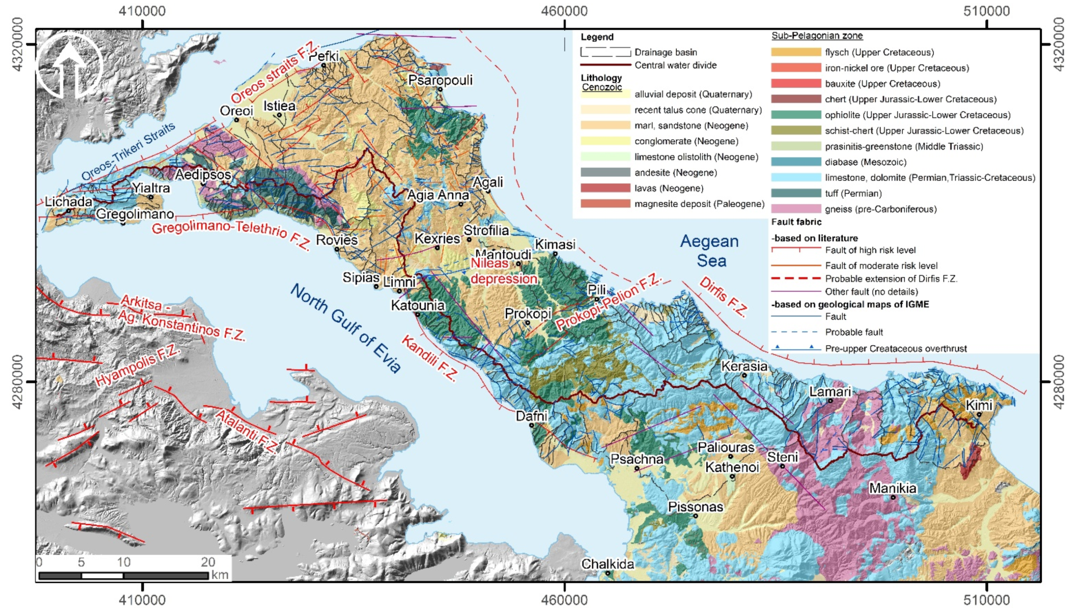
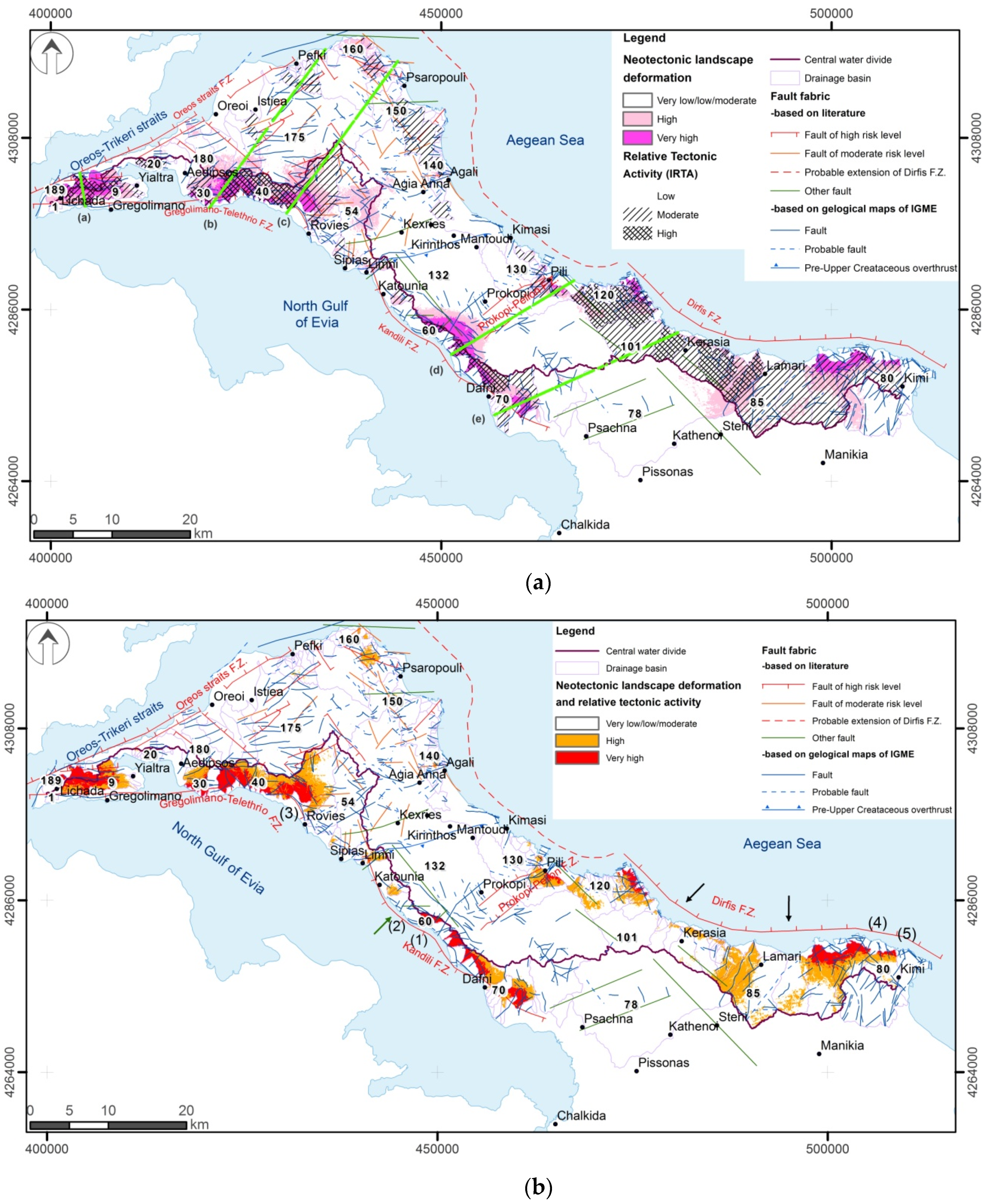
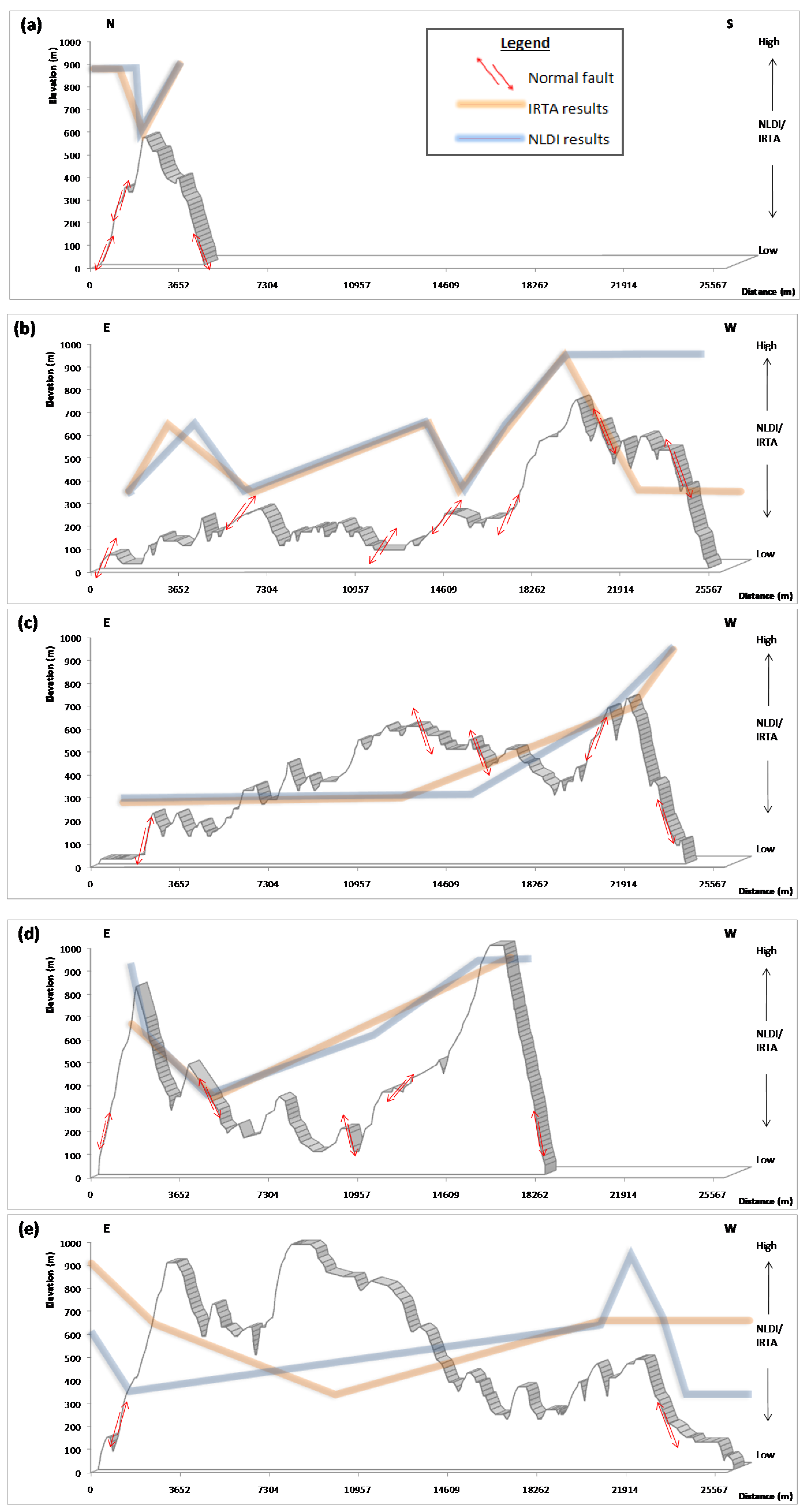
- The results of the neotectonic landscape deformation assessment revealed that the landscape of the most extensive catchments that drain the uplifting block of the Dirfis fault zone (catchments 85 and 101) are characterized by very low values of NLDI, indicating that this offshore fault zone is not continuous but segmented into three discrete portions (the segmentation points/areas are marked with black arrows in Figure 7b). The east segment extends from the eastern termination of the fault to catchment 85 (Figure 9e, location 4), the middle segment lies between the catchments 85 and 101, while the western segment extends from catchment 101 to the western end of the fault zone. This segmentation limits the magnitude of a potential earthquake caused by this fault zone. The Dirfis fault zone terminates to the north at its intersection with the Prokopi–Pelion fault, which has a roughly NE–SW trend and acts as a barrier separating the Dirfis fault zone from its probable extension to the north. North of this area the uplift is limited and the landscape is smoother, indicating low neotectonic deformation. The landscape along the cross-section of the Dirfis fault zone (Figure 8e) and the higher values of the indices at the east and west coasts are indicative of horst morphology in this part of the island.
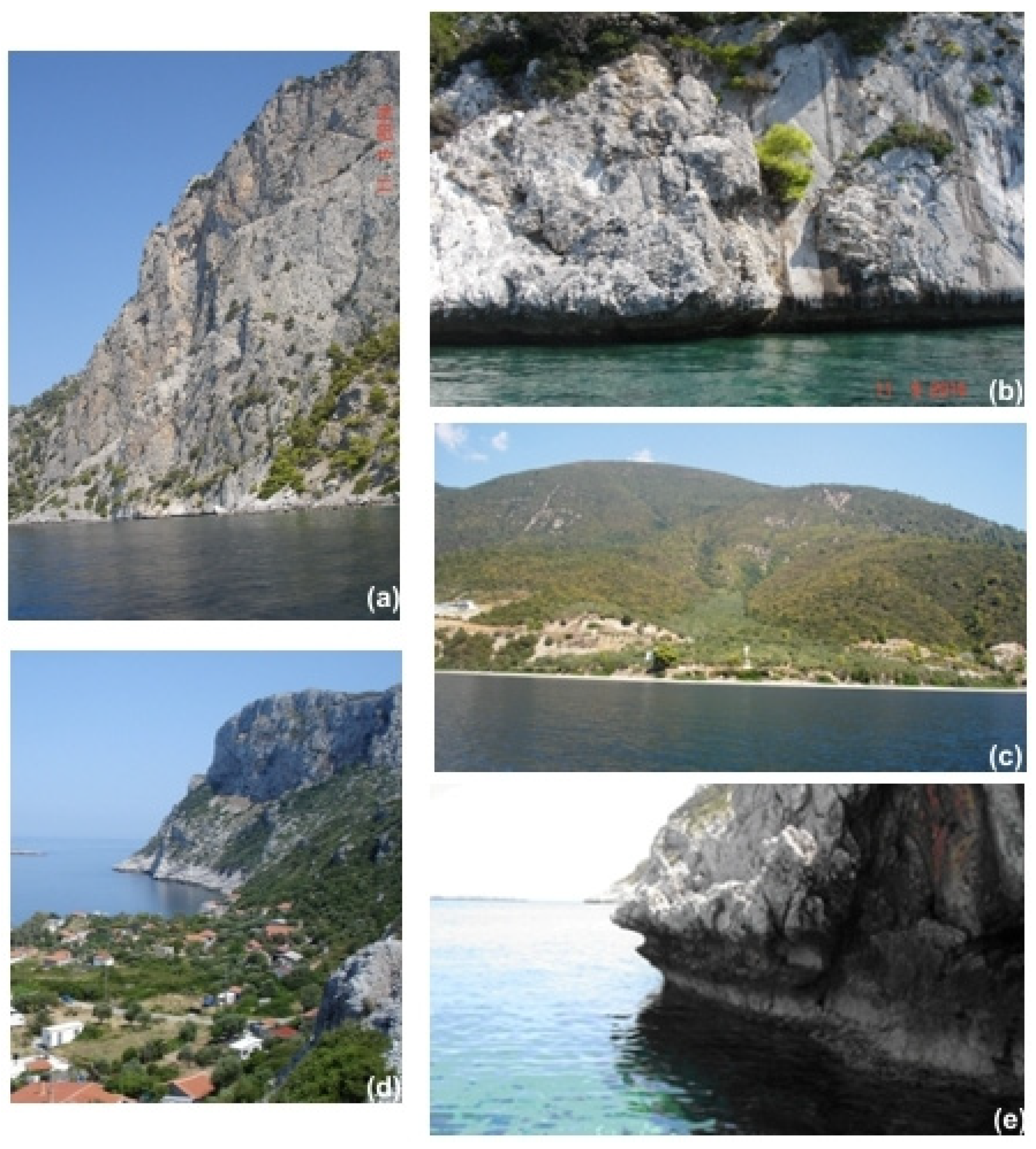
- The Kandili fault zone also seems to be segmented into two portions (green arrow in Figure 7b). The north segment has a length of 22.73 km, whereas the length of the south segment is 8.64 km. A fault that crosses the Kandili fault zone (Figure 9b, location 1) (near drainage basin 60) seems to be responsible for this segmentation. The scarp of this crossing fault has been verified during the fieldwork (Figure 9c, location 2). On the tectonic map of the north Gulf of Evia published by Sakellariou et al. [70], this fault extends northwestward, crossing the Gulf reaching the Ag. Konstantinos fault zone at the opposite coast. According to Palyvos et al. [65], this fault extends eastward up to Kireas stream, north of the Prokopi–Pelion fault zone. The Kandili fault zone cross-section (Figure 8d) shows higher values of both NLDI and IRTA indices at the east and west coasts, which supports the view of a horst morphology at this part of the island. The same stands for the Lichada Peninsula (Figure 8a).
- The Gregolimano–Telethrio fault zone consists of two segments and both seem to be very active based on the degree of the deformation of its footwall landscape (Figure 9d, location 3). The Gregolimano and Telethrio topographic profiles (Figure 8c,d) indicate that both relative tectonic activity and landscape neotectonic deformation increase significantly from east to west. This means that the Gregolimano–Telethrio fault zone shows higher levels of relative neotectonic activity.
- The landscape of the northeast part of the study area is classified as highly deformed. The area south of the drainage basin 160 is affected by a large number of smaller faults of moderate seismic risk level.
6. Conclusions
Author Contributions
Funding
Data Availability Statement
Acknowledgments
Conflicts of Interest
References
- Argyriou, A.V.; Teeuw, R.M.; Rust, D.; Sarris, A. GIS multi-criteria decision analysis for assessment and mapping of neotectonic landscape deformation: A case study from Crete. Geomorphology 2016, 253, 262–274. [Google Scholar] [CrossRef] [Green Version]
- Chen, Y.; Sung, Q.; Cheng, K. Along-strike variations of morphometric features in the western foothills of Taiwan: Tectonic implications based on stream gradient and hypsometric analysis. Geomorphology 2003, 56, 109–137. [Google Scholar] [CrossRef]
- Siddiqui, A.; Soldati, M. Appraisal of active tectonics using DEM-based hypsometric integral and trend surface analysis in Emilia–Romagna Apennines, northern Italy, Turk. J. Earth Sci. 2014, 23, 277–292. [Google Scholar] [CrossRef]
- Kothyari, G.C.; Rastogi, B.K.; Morthekai, P.; Dumka, R.K.; Kandregula, R.S. Active segmentation assessment of the tectonically active South Wagad fault in kachchh, western peninsular India. Geomorphology 2016, 253, 491–507. [Google Scholar] [CrossRef]
- Siddiqui, S.; Castaldini, D.; Soldati, M. DEM-based drainage network analysis using steepness and Hack SL indices to identify areas of differential uplift in Emilia–Romagna Apennines, northern Italy. Arab. J. Geosci. 2017, 10, 3. [Google Scholar] [CrossRef]
- Saber, R.; Isik, V.; Caglayan, A. Tectonic geomorphology of the Aras drainage basin (NW Iran): Implications for the recent activity of the Aras fault zone. Geol. J. 2019, 1–27. [Google Scholar] [CrossRef]
- El Hamdouni, R.; Irigaray, C.; Fernández, T.; Chacón, J.; Keller, E.A. Assessment of relative active tectonics, southwest border of the Sierra Nevada (southern Spain). Geomorphology 2008, 96, 150–173. [Google Scholar] [CrossRef]
- Arian, M.; Aram, Z. Relative tectonic activity classification in the Kermanshah area, western Iran. Solid Earth 2014, 5, 1277–1291. [Google Scholar] [CrossRef] [Green Version]
- Anand, A.K.; Pradhan, S.P. Assessment of active tectonics from geomorphic indices and morphometric parameters in part of Ganga basin. J. Mt. Sci. 2019, 16, 1943–1961. [Google Scholar] [CrossRef]
- Valkanou, K.; Karymbalis, E.; Papanastassiou, D.; Soldati, M.; Chalkias, C.; Gaki-Papanastassiou, K. Morphometric Analysis for the Assessment of Relative Tectonic Activity in Evia Island, Greece. Geosciences 2020, 10, 264. [Google Scholar] [CrossRef]
- Burbank, D.W.; Anderson, R.S. Tectonic Geomorphology, 2nd ed.; Wiley-Blackwell: Hoboken, NJ, USA, 2012. [Google Scholar]
- Karymbalis, E.; Papanastassiou, D.; Gaki-Papanastassiou, K.; Ferentinou, M.; Chalkias, C. Late Quaternary rates of stream incision in Northeast Peloponnese, Greece. Front. Earth Sci. 2016, 10, 455–478. [Google Scholar] [CrossRef]
- Goldsworthy, M.; Jackson, J. Active normal fault evolution in Greece revealed by geomorphology and drainage patterns. J. Geol. Soc. 2000, 157, 967–981. [Google Scholar] [CrossRef]
- Keller, E.A.; Pinter, N. Active Tectonics, Earthquake, Uplift and Landscape, 2nd ed.; Prentice Hall: Upper Saddle River, NJ, USA, 2002. [Google Scholar]
- He, C.; Cheng, Y.; Rao, G.; Chen, P.; Hu, J.; Yu, Y.; Yao, Q. Geomorphological signatures of the evolution of active normal faults along the Langshan Mountains, North China. Geodin. Acta 2018, 30, 163–182. [Google Scholar] [CrossRef]
- Densmore, A.L.; Dawers, N.H.; Gupta, S.; Guidon, R.; Goldin, T. Footwall topographic development during continental extension. J. Geophys. Res. 2001, 109. [Google Scholar] [CrossRef] [Green Version]
- Maroukian, H.; Gaki-Papanastassiou, K.; Karymbalis, E.; Vouvalidis, K.; Pavlopoulos, K.; Papanastassiou, D.; Albanakis, K. Morphotectonic control on drainage network evolution in the Perachora Peninsula, Greece. Geomorphology 2008, 102, 81–92. [Google Scholar] [CrossRef]
- Ntokos, D.; Lykoudi, E.; Rondoyanni, T. Geomorphic analysis in areas of low-rate neotectonic deformation: South Epirus (Greece) as a case study. Geomorphology 2016, 263, 156–169. [Google Scholar] [CrossRef]
- Amine, A.; El Ouardi, H.; Zebari, M.; El Makrini, H. Active tectonics in the Moulay Idriss Massif (South Rifian Ridges, NW Morocco): New insights from geomorphic indices and drainage pattern analysis. J. Afr. Earth Sci. 2020, 167, 103833. [Google Scholar] [CrossRef]
- Jayappa, K.S.; Markose, V.J.; Nagaraju, M. Identification of geomorphic signatures of neotectonic activity using DEM in the precambrian terrain of Western Ghats, India. Int. Arch. Photogramm. Remote Sens. Spatial Inf. Sci. 2012, XXXIX-B8, 215–220. [Google Scholar] [CrossRef] [Green Version]
- Mahmood, S.A.; Gloaguen, R. Appraisal of active tectonics in Hindu Kush: Insights from DEM derived geomorphic indices and drainage analysis. Geosci. Front. 2012, 3, 407–428. [Google Scholar] [CrossRef]
- Alipoor, R.; Poorkerman, M.; Zare, M.; El Hamdouni, R. Active tectonic assessment around Rudbar Lorestan dam site, High Zagros Belt (SW of Iran). Geomorphology 2011, 128, 1–14. [Google Scholar] [CrossRef]
- Tsimi, C.; Ganas, A.; Soulakellis, N.; Kairis, O.; Valmis, S. Morphotectonics of the Psathopyrgos active fault, western Corinth Rift, central Greece. Bull. Geol. Soc. Greece 2007, 40, 500–511. [Google Scholar] [CrossRef] [Green Version]
- Sboras, S.; Ganas, A.; Pavlides, S. Morphotectonic analysis of the neotectonic and active faults of Beotia (central Greece) using GIS techniques. Bull. Geol. Soc. Greece 2010, 43, 1607–1618. [Google Scholar] [CrossRef] [Green Version]
- Dar, R.A.; Romshoo, S.A.; Chandra, R.; Ahmad, I. Tectono-geomorphic study of the Karewa Basin of Kashmir Valley. J. Asian Earth Sci. 2014, 92, 143–156. [Google Scholar] [CrossRef]
- Annayat, W.; Sil, B.S. Assessing channel morphology and prediction of centerline channel migration of the Barak River using geospatial techniques. Bull. Eng. Geol. Environ. 2020, 79. [Google Scholar] [CrossRef]
- Bhatt, S.C.; Singh, R.; Ansari, M.A.; Bhatt, S. Quantitative Morphometric and Morphotectonic Analysis of Pahuj Catchment Basin, Central India. J. Geol. Soc. India 2020, 96, 513–520. [Google Scholar] [CrossRef]
- Del Val, M.; Iriarte, E.; Arriolabengoa, M.; Aranburu, A. An automated method to extract fluvial terraces from LIDAR based high resolution Digital Elevation Models: The Oiartzun valley, a case study in the Cantabrian Margin. Quat. Int. 2015, 364, 35–43. [Google Scholar] [CrossRef]
- Kamiński, M. DTM-based analysis of the spatial distribution of topolineaments. Open Geosci. 2020, 12, 1185–1199. [Google Scholar] [CrossRef]
- Székely, B.; Zámolyi, A.; Draganits, E.; Briese, C. Geomorphic expression of neotectonic activity in a low relief area in an Airborne Laser Scanning DTM: A case study of the Little Hungarian Plain (Pannonian Basin). Tectonophysics 2009, 474, 353–366. [Google Scholar] [CrossRef]
- Rashidi, A.; Abbasi, M.-R.; Nilfouroushan, F.; Shafiei, S.; Derakhshani, R.; Nemati, M. Morphotectonic and earthquake data analysis of interactional faults in Sabzevaran Area, SE Iran. J. Struct. Geol. 2020, 139, 104147:1–104147:20. [Google Scholar] [CrossRef]
- Guo, J.; Xu, S.; Fan, H. Neotectonic interpretations and PS-InSAR monitoring of crustal deformations in the Fujian area of China. Open Geosci. 2017, 9, 126–132. [Google Scholar] [CrossRef]
- Parcharidis, I.; Kourkouli, P.; Karymbalis, E.; Foumelis, M.; Karathanassi, V. Time Series Synthetic Aperture Radar Interferometry for Ground Deformation Monitoring over a Small Scale Tectonically Active Deltaic Environment (Mornos, Central Greece). J. Coast. Res. 2013, 29, 325–338. [Google Scholar] [CrossRef] [Green Version]
- Elmahdy, S.I.; Mohamed, M.M. Mapping of tecto-lineaments and investigate their association with earthquakes in Egypt: A hybrid approach using remote sensing data. Geomat. Nat. Hazards Risk 2016, 7, 600–619. [Google Scholar] [CrossRef] [Green Version]
- Kusák, M.; Vilímek, V.; Minár, J. Influence of neotectonics on land surface evolution in the upper part of the Blue Nile Basin (Ethiopia): Findings from a DEM. AUC Geogr. 2019, 54, 129–151. [Google Scholar] [CrossRef] [Green Version]
- Smith, M.J.; Clark, C.D. Methods for the visualization of digital elevation models for landform mapping. Earth Surf. Process. Landf. 2005, 30, 885–900. [Google Scholar] [CrossRef]
- Ruzinoor, C.M.; Shariff, A.R.M.; Pradhan, B.; Rodzi Ahmad, M.; Rahim, M.S.M. A review on 3D terrain visualization of GIS data: Techniques and software. Geo-Spat. Inf. Sci. 2012, 15, 105–115. [Google Scholar] [CrossRef]
- Sharma, S.A. Application of TecDEM in morphometric studies of Imphal River. Am. Int. J. Res. Sci. Technol. Eng. Math. 2014, 7, 238–243. [Google Scholar]
- Petrovszki, J.; Timár, G. Channel sinuosity of the Körös River system, Hungary/Romania, as possible indicator of the neotectonic activity. Geomorphology 2010, 112, 223–230. [Google Scholar] [CrossRef]
- Bagha, N.; Arian, M.; Ghorashi, M.; Pourkermani, M.; El Hamdouni, R.; Solgi, A. Evaluation of relative tectonic activity in the Tehran basin, central Alborz, northern Iran. Geomorphology 2014, 213, 66–87. [Google Scholar] [CrossRef]
- Whitney, B.B.; Hengesh, J.V. Geomorphological evidence of neotectonic deformation in the Carnarvon Basin, Western Australia. Geomorphology 2015, 228, 579–596. [Google Scholar] [CrossRef] [Green Version]
- Gasparini, N.M.; Fischer, G.C.; Adams, J.M.; Dawers, N.H.; Janoff, A.M. Morphological signatures of normal faulting in low-gradient alluvial rivers in south-eastern Louisiana, USA. Earth Surf. Process. Landf. 2016, 41, 642–657. [Google Scholar] [CrossRef]
- Ahmad, S.; Alam, A.; Ahmad, B.; Afzal, A.; Bhat, M.I.; Bhat, M.S.; Ahmad, H.F. Tectono-geomorphic indices of the Erin basin, NE Kashmir Valley, India. J. Asian Earth Sci. 2018, 151, 16–30. [Google Scholar] [CrossRef]
- Rozos, D.; Bathrellos, D.G.; Skilodimou, D.H. Landslide susceptibility mapping of the northeastern part of Achaia Prefecture using Analytical Hierarchical Process and GIS techniques. Bull. Geol. Soc. Greece 2010, XLIII, 1637–1646. [Google Scholar] [CrossRef] [Green Version]
- Elsheikh, R.F.A.; Ouerghi, S.; Elhag, A.R. Flood Risk Map Based on GIS, and Multi Criteria Techniques (Case Study Terengganu Malaysia). J. Geogr. Inf. Syst. 2015, 7, 348–357. [Google Scholar] [CrossRef] [Green Version]
- Bathrellos, G.; Karymbalis, E.; Skilodimou, H.; Gaki-Papanastassiou, K.; Baltas, E. Urban flood hazard assessment in the basin of Athens Metropolitan city, Greece. Environ. Earth Sci. 2016, 75, 319:1–319:14. [Google Scholar] [CrossRef]
- Della Seta, M.; Del Monte, M.; Fredi, P.; Lupia Palmieri, E. Quantitative morphotectonic analysis as a tool for detecting deformation patterns in soft-rock terrains: A case study from the southern Marches, Italy. Géomorphol. Relief Process. Environ. 2004, 10, 267–284. [Google Scholar] [CrossRef]
- Lone, A. Morphometric and Morphotectonic Analysis of Ferozpur Drainage Basin Left Bank Tributary of River Jhelum of Kashmir Valley, NW Himalayas, India. J. Geogr. Nat. Disasters 2017, 7, 1000208:1–1000208:8. [Google Scholar] [CrossRef]
- Charizopoulos, N.; Mourtzios, P.; Psilovikos, T.; Psilovikos, A.; Karamoutsou, L. Morphometric analysis of the drainage network of Samos Island (northern Aegean Sea): Insights into tectonic control and flood hazards. Comptes Rendus Geosci. 2019, 351, 375–383. [Google Scholar] [CrossRef]
- Ayaz, S.; Dhali, M.K. Longitudinal profiles and geomorphic indices analysis on tectonic evidence of fluvial form, process and landform deformation of Eastern Himalayan Rivers, India. Geol. Ecol. Landsc. 2020, 4, 11–22. [Google Scholar] [CrossRef] [Green Version]
- Davoli, L.; Fredi, P.; Russo, F.; Troccoli, A. Natural and anthropogenic factors of flood hazards in the Somma-Vesuvius area (Italy)/Rôle des facteurs naturels et anthropiques sur les risques d’inondation autour du Vésuve-Somma (Italie). Géomorphol. Relief Process. Environ. 2001, 7, 195–207. [Google Scholar] [CrossRef]
- Glennon, A.; Groves, C. An examination of perennial stream drainage patterns within the Mammoth Cave watershed, Kentucky. J. Cave Karst Stud. 2002, 64, 82–91. [Google Scholar]
- Sreedevi, P.D.; Owais, S.; Khan, H.H.; Ahmed, S. Morphometric Analysis of a Watershed of South India Using SRTM Data and GIS. J. Geol. Soc. India 2009, 73, 543–552. [Google Scholar] [CrossRef]
- Evans, I.S. An integrated system of terrain analysis and slope mapping. Z. Geomorphol. Suppl. Stuttg. 1980, 36, 274–295. [Google Scholar]
- Burrough, P.A. Principles of Geographical Information system for Land Resource Assessment, 1st ed.; Clarendon Press: Oxford, UK, 1986. [Google Scholar] [CrossRef]
- Beven, K.J.; Kirkby, M.J. A physically based variable contributing area model of basin hydrology. Hydrol. Sci. Bull. 1979, 24, 43–69. [Google Scholar] [CrossRef] [Green Version]
- Sørensen, R.; Zinko, U.; Seibert, J. On the calculation of the topographic wetness index: Evaluation of different methods based on field observations. Hydrol. Earth Syst. Sci. 2006, 10, 101–112. [Google Scholar] [CrossRef] [Green Version]
- Karcz, I. Rapid determination of lineament and joint densities. Tectonophysics 1978, 44, T29–T33. [Google Scholar] [CrossRef]
- Mountrakis, D.M. Geology of Greece; University Studio Press: Thessaloniki, Greece, 1985. (In Greek) [Google Scholar]
- Mettos, A.; Rondogianni, T.; Papadakis, G.; Paschos, P.; Georgiou, C. New geological data of the neogene deposits of N.Euboea. Bull. Geol. Soc. Greece 1991, 25, 71–83. (In Greek) [Google Scholar]
- Galanakis, D.; Pavlides, S.V.; Mountrakis, D.Μ. Recent brittle tectonic in Almyros—Pagasitikos—Maliakos, N. Euboia & Pilio. Bull. Geol. Soc. Greece 1998, 32, 263–273. (In Greek) [Google Scholar]
- Chousianitis, K.; Ganas, A.; Gianniou, M. Kinematic interpretation of present-day crustal deformation in central Greece from continuous GPS measurements. J. Geodyn. 2013, 71, 1–13. [Google Scholar] [CrossRef]
- Goldsworthy, M.; Jackson, J.; Haines, J. The continuity of active fault systems in Greece. Geophys. J. Int. 2002, 148, 596–618. [Google Scholar] [CrossRef] [Green Version]
- Roberts, S.; Jackson, J. Active normal faulting in central Greece: An overview. In The Geometry of Normal Faults; Roberts, A.M., Yielding, G., Freeman, B., Eds.; Geological Society Sp. Pub.56: London, UK, 1991; pp. 125–142. [Google Scholar] [CrossRef]
- Palyvos, N.; Bantekas, I.; Kranis, H. Transverse fault zones of subtle geomorphic signature in northern Evia island (central Greece extensional province): An introduction to the Quaternary Nileas graben. Geomorphology 2006, 76, 363–374. [Google Scholar] [CrossRef]
- Valkanou, K.; Karymbalis, E.; Papanastassiou, D.; Gaki-Papanastassiou, K.; Giles, P. Analysis of relationships among coastal alluvial fans and their contributing catchments in North Evoikos Gulf (Central Greece). Bull. Geol. Soc. Greece 2013, XLVII, 344–355. [Google Scholar] [CrossRef]
- Genre, C. Néotectonique et développement des terrasses de l’Holocène récent: L’exemple de l’Eubée (Grèce centreorientale)/Neotectonics and Late Holocene terraces. The example of Euboea (Central Eastern Greece). Géomorphol. Relief Process. Environ. 1999, 5, 143–158. [Google Scholar]
- Stiros, S.C.; Arnold, M.; Pirazolli, P.A.; Laborel, J.; Laborel, F.; Papageorgiou, S. Historical cosesmic uplift on Euboea island, Greece. Earth Planet. Sci. Lett. 1992, 108, 109–117. [Google Scholar] [CrossRef]
- Evelpidou, Ν.; Vassilopoulos, A.; Pirazzoli, P.A. Holocene emergence in Euboea island (Greece). Mar. Geol. 2012, 295–298, 14–19. [Google Scholar] [CrossRef]
- Sakellariou, D.; Rousakis, G.; Kaberi, H.; Kapsimalis, V.; Georgiou, P.; Kanellopoulos, T.; Lykousis, V. Tectono-sedimentary structure and Late Quaternary evolution of the North Evia Gulf basin, central Greece: Preliminary results. Bull. Geol. Soc. Greece 2007, 40, 451–462. [Google Scholar] [CrossRef]
- Papanastassiou, D.; Lataoussakis, J.; Stavrakakis, G. A revised catalogue of earthquakes in the broader area of Greece for the period 1950–2000. Bull. Geol. Soc. Greece 2001, XXXIV, 1563–1566. [Google Scholar] [CrossRef] [Green Version]
- Chalkias, C.; Papanastassiou, D.; Karymbalis, E.; Chalkias, G. Maximum macroseismic intensity map of Greece for the time period 1953–2011. J. Maps 2014, 10, 195–202. [Google Scholar] [CrossRef]
- Pantosti, D.; De Martini, P.M.; Papanastassiou, D.; Lemeille, F.; Palyvos, N.; Stavrakakis, G. Paleoseismological trenching across the Atalanti fault (Central Greece): Evidence for the ancestors of the 1894 earthquake during Middle Age and Roman time. Bull. Seismol. Soc. Am. 2004, 94, 531–549. [Google Scholar] [CrossRef]
- IGME. Geological map of Greece, Scale 1:50.000. Steni-Dhirfios, Psachna-Pilion, Pelasgia-Myli, Limni, Larimna, Kimi, Istiaia Sheets; Institute of Geology and Mineral Exploration: Athens, Greece, 1957–1984. [Google Scholar]
- Ganas, A.; Oikonomou, I.A.; Tsimi, C. NOAfaults: A digital database for active faults in Greece. Chania. Bull. Geol. Soc. Greece 2013, 47, 518–530. [Google Scholar] [CrossRef] [Green Version]
- Genre, C. Cartes des lineaments structuraux établies à partir d’images Landsat II et des données sismotectoniques OASP et IGME; Rapport de recherché; CIEM: Poitiers, France, 1985. [Google Scholar]
- Gautier, P. Géométrie crustale et cinématique de l’extension tardi-orogénique dans le domaine centre-égéen (Iles des Cyclades et d’Eubée, Grèce). Ph.D. Thesis, Géosciences Rennes, Université de Rennes, Rennes, France, 1995. [Google Scholar]
- Popovic, A. Analyse Morphostructurale sur un Exemple de Bloc Basculé d’échelle Crustale (l’île ď Eubée, Grèce) dans une Région ď Extension Active (Grèce Centrale); Mémoire de DEA Géosciences Rennes, Tectonique: Rennes, France, 1996; p. 12. [Google Scholar]
- Drobne, S.; Lisec, A. Multi-attribute Decision Analysis in GIS: Weighted Linear Combination and Ordered Weighted Averaging. Informatica 2009, 33, 459–474. [Google Scholar]
- Kontos, T.D.; Komilis, D.P.; Halvadakis, C.P. Siting MSW landfills with a spatial multiple criteria analysis methodology. Waste Manag. 2005, 25, 818–832. [Google Scholar] [CrossRef]
- Papadopoulos, A.G.; Chalkias, C.; Faka, A. The re-examination of the Greek countryside through a dynamic methodological approach and geographical information systems. Greek Rev. Soc. Res. 2016, 125, 99–129. (In Greek) [Google Scholar]
- Chalkias, C. Geographical Analysis with the Use of Geoinformatics. Athens, 2015, Hellenic Academic Libraries Link (in Greek). Available online: https://repository.kallipos.gr/handle/11419/4546 (accessed on 5 August 2020).
- Glock, W.S. Available Relief as a Factor of Control in the Profile of a Landform. J. Geogr. 1932, 40, 74–83. [Google Scholar] [CrossRef]
- Raisz, E.; Henry, J. An Average Slope Map of Southern New England. Geogr. Rev. 1937, 27, 467–472. [Google Scholar] [CrossRef]
- Troiani, F.; Della Seta, M. The use of the Stream Length–Gradient index in morphotectonic analysis of small catchments: A case study from Central Italy. Geomorphology 2008, 102, 159–168. [Google Scholar] [CrossRef]
- Ciccacci, S.; De Rita, D.; Fredi, P. Quantitative Geomorphology and Morphoneotectonics of the Morlupo-Castelnuovo di Porto (Monti Sabatini, Latium). Suppl. Geogr. Fis. Din. Quat. 1988, I, 197–206. [Google Scholar]
- Ciotoli, G.; Della Seta, M.; Del Monte, M.; Fredi, P.; Lombardi, S.; Lupia Palmieri, E.; Pugliese, F. Morphological and geochemical evidence of neotectonics in the volcanic area of Monti Vulsini (Latium, Italy). Quat. Int. 2003, 101–102, 103–113. [Google Scholar] [CrossRef]
- Thakurdesai, S.C.; Pise, S.K. A Study of Relief and Slope of Upper Kundalika River Basin, Raigad, Maharashtra. Int. J. Interdiscip. Res. Sci. Soc. Cult. (Ijirssc) 2016, 2, 391–399. [Google Scholar]
- Hack, J.T. Stream-profile analysis and stream-gradient index. J. Res. U.S. Geol. Surv. 1973, 1, 421–429. [Google Scholar]
- Pérez-Peña, J.V.; Azañón, J.M.; Azor, A.; Delgado, J.; González-Lodeiro, F. Spatial analysis of stream power using GIS: SLk anomaly maps. Earth Surf. Process. Landf. 2009, 34, 16–25. [Google Scholar] [CrossRef]
- Seeber, L.; Gornitz, V. River profiles along the Himalayan arc as indicators of active tectonics. Tectonophysics 1983, 92, 335–367. [Google Scholar] [CrossRef]
- Horton, R.E. Erosional development of streams and their drainage basins; hydrophysical approach to quantitative morphology. Geol. Soc. Am. Bull. 1945, 56, 275–370. [Google Scholar] [CrossRef] [Green Version]
- Han, Z.; Wu, L.; Ran, Y.; Ye, Y. The concealed active tectonics and their characteristics as revealed by drainage density in the North China plain (NCP). J. Asian Earth Sci. 2003, 21, 989–998. [Google Scholar] [CrossRef]
- Mrinalinee Devi, R.K.; Bhakuni, S.S.; Bora, P.K. Tectonic implication of drainage set-up in the Sub-Himalaya: A case study of Papumpare district, Arunachal Himalaya, India. Geomorphology 2011, 127, 14–31. [Google Scholar] [CrossRef]
- Resmi, M.R.; Babeesh, C.; Achyutham, H. Quantitative analysis of the drainage and morphometric characteristics of the Palar River basin, Southern Peninsular India; using bAd calculator (bearing azimuth and drainage) and GIS. Geol. Ecol. Landsc. 2019, 3, 295–307. [Google Scholar]
- Parveen, R.; Kumar, U.; Singh, V.K. Geomorphometric Characterization of Upper South Koel Basin, Jharkhand: A Remote Sensing & GIS Approach. J. Water Resour. Prot. 2012, 4, 1042–1050. [Google Scholar] [CrossRef] [Green Version]
- Kouli, M.; Vallianatos, F.; Soupios, P.; Alexakis, D. Gis-based morphometric analysis of two major watersheds, Western Crete, Greece. J. Environ. Hydrol. 2007, 15, 1–17. [Google Scholar]
- Kokinou, Ε.; Skilodimou, H.; Bathrellos, G. Morphotectonic analysis of Heraklion Basin (Crete, Greece). Bull. Geol. Soc. Greece 2013, 47, 285–294. [Google Scholar] [CrossRef] [Green Version]
- Quinn, P.; Beven, K.; Chevallier, P.; Planchon, O. The prediction of hillslope paths for distributed hydrological modeling using digital terrain models. Hydrol. Process. 1994, 5, 59–79. [Google Scholar] [CrossRef]
- Schmidt, F.; Persson, A. Comparison of DEM Data Capture and Topographic Wetness Indices. Precis. Agric. 2003, 4, 179–192. [Google Scholar] [CrossRef]
- Migoń, P.; Kasprzak, M.; Traczyk, A. How high-resolution DEM based on airborne LiDAR helped to reinterpret landforms—Examples from the Sudetes, SW Poland. Landf. Anal. 2013, 22, 89–101. [Google Scholar] [CrossRef]
- Tagil, S.; Jenness, J. GIS-Based Automated Landform Classification and Topographic Landcover and Geologic Attributes of Landforms Around the Yazoren Polje, Turkey. J. Appl. Sci. 2008, 8, 910–921. [Google Scholar] [CrossRef] [Green Version]
- Ganas, A.; Pavlides, S.; Karastathis, V. DEM-based morphometry of range-front escarpments in Attica, central Greece, and its relation to fault slip rates. Geomorphology 2005, 65, 301–319. [Google Scholar] [CrossRef]
- Abdullah, A.; Akhir, J.M.; Abdullah, I. The Extraction of Lineaments Using Slope Image Derived from Digital Elevation Model: Case Study of Sungai Lembing—Maran area, Malaysia. J. Appl. Sci. Res. 2010, 6, 1745–1751. [Google Scholar]
- Chandrasekhar, P.; Martha, T.R.; Venkateswarlu, N.; Kamaraju, M.V.V. Regional geological studies over parts of Deccan Syneclise using remote sensing and geophysical data for understanding hydrocarbon prospects. Curr. Sci. 2011, 100, 95–99. [Google Scholar]
- Masoud, A.A.; Koike, K. Auto-detection and integration of tectonically significant lineaments from SRTM DEM and remotely-sensed geophysical data. Isprs J. Photogramm. Remote Sens. 2011, 66, 818–832. [Google Scholar] [CrossRef]
- Hung, L.Q.; Dinh, N.Q.; Batelaan, O.; Tam, V.T.; Lagrou, D. Remote sensing and GIS-based analysis of cave development in the Suoimuoi Catchment (Son La—NW Vietnam). J. Cave Karst Stud. 2002, 64, 23–33. [Google Scholar]
- Sajadi, P.; Singh, A.; Mukherjee, S.; Chapi, K. Influence of structural lineaments on drainage morphometry in Qorveh-Dehgolan basin, Kurdistan, Iran. Geocarto Int. 2019, 35, 1722–1749. [Google Scholar] [CrossRef]
- Marinos, P.; Hoek, E. GSI: A geologically friendly tool for rock mass strength estimation. In Proceedings of the GeoEng 2000, Melbourne, Australia, 19–24 November 2000. [Google Scholar]
- IGME. Geotechnical Map of Greece, Scale 1:500.000; Institute of Geology and Mineral Exploration: Athens, Greece, 1993. [Google Scholar]
- Saaty, T.L. The Analystic Hierarchy Process: Planning, Priority Setting, Resource Allocation; Mcgraw-Hill: New York, NY, USA, 1980. [Google Scholar]
- Malczewski, J. GIS-based multicriteria decision analysis: A survey of the literature. Int. J. Geogr. Inf. Sci. 2006, 20, 703–726. [Google Scholar] [CrossRef]
- Saaty, T.L. Decision making with the analytic hierarchy process. Int. J. Serv. 2008, 1, 83–98. [Google Scholar] [CrossRef] [Green Version]
- Saaty, T.L.; Vargas, L. Prediction, Projection and Forecasting; Kluwer Academic Publishers: Dordrecht, The Netherlands, 1991. [Google Scholar]
- Samal, D.R.; Gedam, S.S.; Nagarajan, R. GIS based drainage morphometry and its influence on hydrology in parts of Western Ghats region, Maharashtra, India. Geocarto Int. 2015, 30, 755–778. [Google Scholar] [CrossRef]
- Malczewski, J. Gis and Multicriteria Decision Analysis; John Wiley & Sons Inc.: New York, NY, USA, 1999. [Google Scholar]
- Ayalew, L.; Yamagishi, H.; Ugawa, N. Landslide susceptibility mapping using GIS-based weighted linear combination, the case in Tsugawa area of Agano River, Niigata Prefecture, Japan. Landslides 2004, 1, 73–81. [Google Scholar] [CrossRef]
- Leontaris, S.; Delibasis, Ν. Vertical movements of the island Eubea based on geomorphological and seismotectonic observations. In Proceedings of the 1st Panhellenic Geographical Conference, Athens, Greece, 20–22 February 1987; pp. 68–100. (In Greek). [Google Scholar]
- Dubey, R.K.; Dar, J.A.; Kothyari, G.C. Evaluation of relative tectonic perturbations of the Kashmir Basin, Northwest Himalaya, India: An integrated morphological approach. J. Asian Earth Sci. 2017, 148, 153–172. [Google Scholar] [CrossRef]


| a11 | a12 | … | a1n |
| a21 | a22 | … | a2n |
| … | |||
| an1 | an2 | … | ann |
| Sum_1 | Sum_2 | … | Sum_n |
| Weighting coefficient (wi) | |||||
| a11/Sum_1 | a12/Sum_2 | … | a1n/Sum_n | Row_sum1 | Row_sum1/n |
| a21/Sum_1 | a22/Sum_2 | … | a2n//Sum_n | Row_sum2 | Row_sum2/n |
| … | … | ||||
| an1/Sum_1 | an2/Sum_2 | … | ann/Sum_n | Row_sumn | Row_sumn/n |
| WV1 = a11*w1 + a12*w2 + … + a1n*wn |
| WV2 = a21*w1 + a22*w2 + … + a2n*wn |
| … |
| WVm = an1*w1 + an2*w2 + … + ann*wn |
| Step a | ||||||||||||
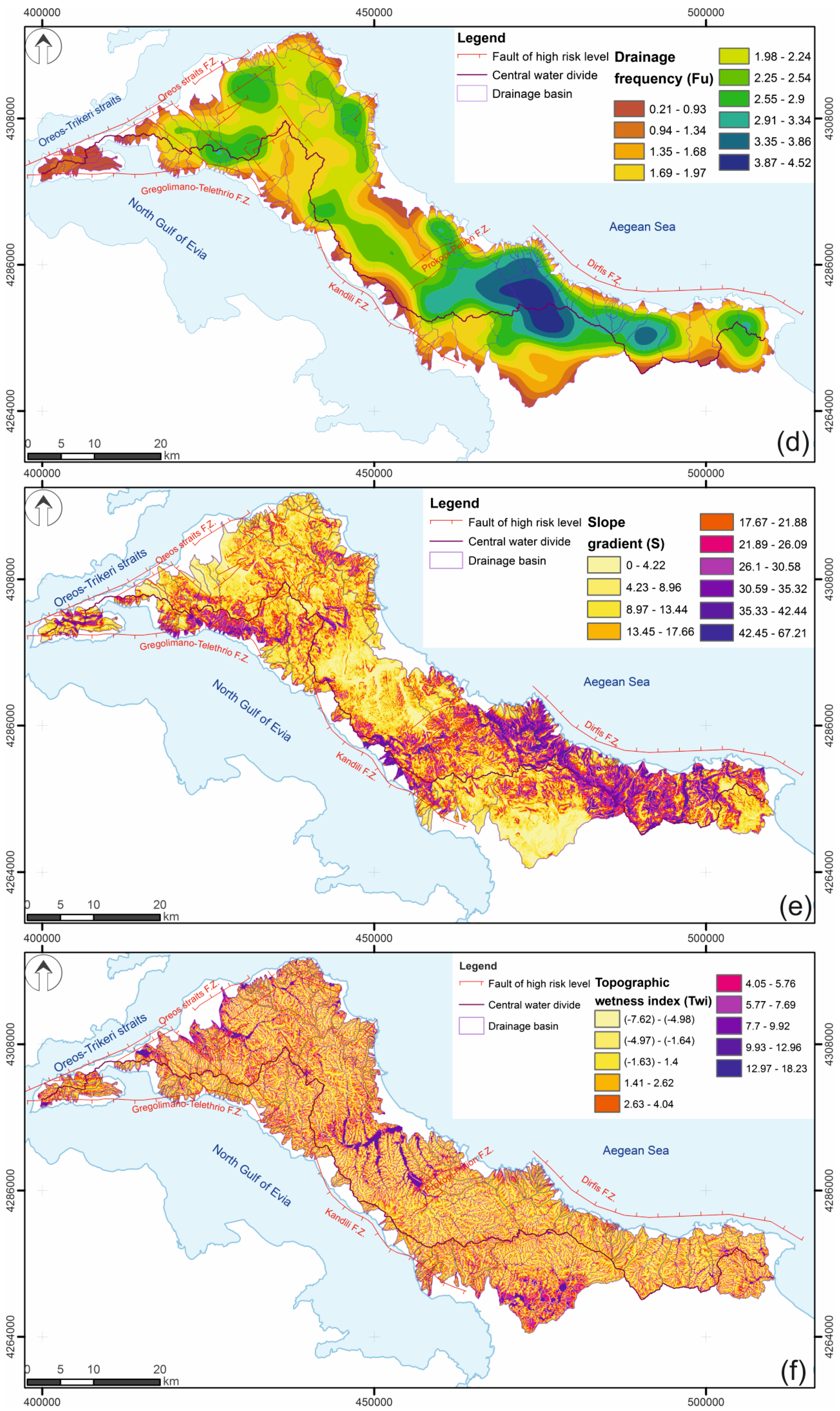
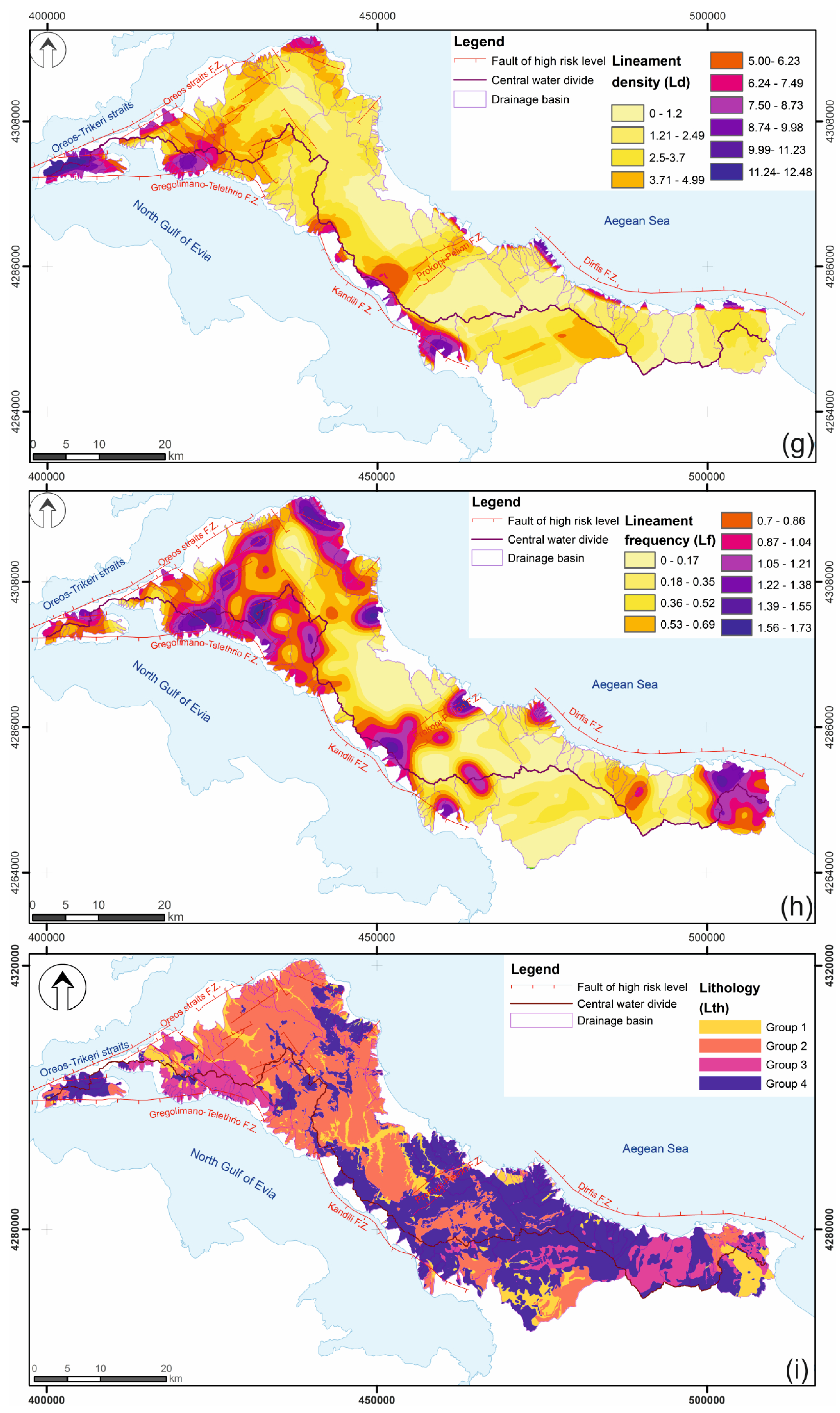
| Ar | SLk | Ld | Lf | Dd | Fu | S | Twi | Lth | ||||
| Ar | 1 | 1 | 2 | 2 | 3 | 3 | 3 | 6 | 5 | |||
| SLk | 1 | 1 | 2 | 2 | 3 | 3 | 3 | 6 | 5 | |||
| Ld | 0.5 | 0.50 | 1 | 1 | 3 | 3 | 3 | 5 | 3 | |||
| Lf | 0.5 | 0.50 | 1 | 1 | 3 | 3 | 3 | 5 | 3 | |||
| Dd | 0.33 | 0.3 | 0.33 | 0.33 | 1 | 1 | 1 | 3 | 4 | |||
| Fu | 0.33 | 0.3 | 0.33 | 0.33 | 1 | 1 | 1 | 3 | 4 | |||
| S | 0.33 | 0.33 | 0.33 | 0.33 | 1 | 1 | 1 | 2 | 4 | |||
| Twi | 0.17 | 0.17 | 0.20 | 0.20 | 0.3 | 0.33 | 0.50 | 1 | 3 | |||
| Lth | 0.20 | 0.20 | 0.33 | 0.33 | 0.25 | 0.25 | 0.25 | 0.33 | 1 | |||
| Sum | 4.37 | 4.37 | 7.53 | 7.53 | 15.58 | 15.58 | 15.75 | 31.33 | 32.00 | |||
| Step b–c | ||||||||||||
| Ar | SLk | Ld | Lf | Dd | Fu | S | Twi | Lth | Sum | |||
| Ar | 0.23 | 0.23 | 0.27 | 0.27 | 0.19 | 0.19 | 0.19 | 0.19 | 0.16 | 1.91 | ||
| SLk | 0.23 | 0.23 | 0.27 | 0.27 | 0.19 | 0.19 | 0.19 | 0.19 | 0.16 | 1.91 | ||
| Ld | 0.11 | 0.11 | 0.13 | 0.13 | 0.19 | 0.19 | 0.19 | 0.16 | 0.09 | 1.32 | ||
| Lf | 0.11 | 0.11 | 0.13 | 0.13 | 0.19 | 0.19 | 0.19 | 0.16 | 0.09 | 1.32 | ||
| Dd | 0.08 | 0.08 | 0.04 | 0.04 | 0.06 | 0.06 | 0.06 | 0.10 | 0.13 | 0.65 | ||
| Fu | 0.08 | 0.08 | 0.04 | 0.04 | 0.06 | 0.06 | 0.06 | 0.10 | 0.13 | 0.65 | ||
| S | 0.08 | 0.08 | 0.04 | 0.04 | 0.06 | 0.06 | 0.06 | 0.06 | 0.13 | 0.62 | ||
| Twi | 0.04 | 0.04 | 0.03 | 0.03 | 0.02 | 0.02 | 0.03 | 0.03 | 0.09 | 0.33 | ||
| Lth | 0.05 | 0.05 | 0.04 | 0.04 | 0.02 | 0.02 | 0.02 | 0.01 | 0.03 | 0.27 | ||
| Sum | 1.00 | 1.00 | 1.00 | 1.00 | 1.00 | 1.00 | 1.00 | 1.00 | 1.00 | |||
| Step d | CR Calculation | |||||||||||
| W | W | WV | C | λ | CI | CR | ||||||
| Ar | 0.21 | Ar | 0.21 | 2.026 | 9.5350 | 9.4642 | 0.0580 | 0.0400 | ||||
| SLk | 0.21 | SLk | 0.21 | 2.026 | 9.5350 | |||||||
| Ld | 0.15 | Ld | 0.15 | 1.423 | 9.6763 | |||||||
| Lf | 0.15 | Lf | 0.15 | 1.423 | 9.6763 | |||||||
| Dd | 0.07 | Dd | 0.07 | 0.684 | 9.4150 | |||||||
| Fu | 0.07 | Fu | 0.07 | 0.684 | 9.4150 | |||||||
| S | 0.07 | S | 0.07 | 0.647 | 9.3681 | |||||||
| Twi | 0.04 | Twi | 0.04 | 0.339 | 9.2619 | |||||||
| Lth | 0.03 | Lth | 0.03 | 0.279 | 9.2954 | |||||||
| Sum | 1.00 | Sum | 85.178 | |||||||||
| F. | W. | C. | R.V. | S.R. | F. | W. | C. | R.V. | S.R. | ||||
| (Ar) | 0.21 | 500.1 | – | 798 | 10 | 100 | (S) | 0.07 | 42.45 | – | 67.21 | 10 | 100 |
| 450.1 | – | 500 | 9 | 90 | 35.33 | – | 42.44 | 9 | 90 | ||||
| 400.1 | – | 450 | 8 | 80 | 30.59 | – | 35.32 | 8 | 80 | ||||
| 350.1 | – | 400 | 7 | 70 | 26.10 | – | 30.58 | 7 | 70 | ||||
| 300.1 | – | 350 | 6 | 60 | 21.89 | – | 26.09 | 6 | 60 | ||||
| 250.1 | – | 300 | 5 | 50 | 17.67 | – | 21.88 | 5 | 50 | ||||
| 200.1 | – | 250 | 4 | 40 | 13.45 | – | 17.66 | 4 | 40 | ||||
| 150.1 | – | 200 | 3 | 30 | 8.97 | – | 13.44 | 3 | 30 | ||||
| 100.1 | – | 150 | 2 | 20 | 4.23 | – | 8.96 | 2 | 20 | ||||
| 13.3 | – | 100 | 1 | 10 | 0 | – | 4.22 | 1 | 10 | ||||
| (SLk) | 0.21 | 22.5 | – | 24.99 | 10 | 100 | (Twi) | 0.04 | (−7.62) | – | (−4.98) | 10 | 100 |
| 20 | – | 22.49 | 9 | 90 | (−4.97) | – | (−1.64) | 9 | 90 | ||||
| 17.5 | – | 19.99 | 8 | 80 | (−1.63) | – | 1.4 | 8 | 80 | ||||
| 15 | – | 17.49 | 7 | 70 | 1.41 | – | 2.62 | 7 | 70 | ||||
| 12.5 | – | 14.99 | 6 | 60 | 2.63 | – | 4.04 | 6 | 60 | ||||
| 10.01 | – | 12.49 | 5 | 50 | 4.05 | – | 5.76 | 5 | 50 | ||||
| 7.51 | – | 10 | 4 | 40 | 5.77 | – | 7.69 | 4 | 40 | ||||
| 5.01 | – | 7.5 | 3 | 30 | 7.70 | – | 9.92 | 3 | 30 | ||||
| 2.51 | – | 5 | 2 | 20 | 9.93 | – | 12.96 | 2 | 20 | ||||
| 0 | – | 2.5 | 1 | 10 | 12.97 | – | 18.23 | 1 | 10 | ||||
| (Dd) | 0.07 | 0 | – | 0.53 | 10 | 100 | (Ld) | 0.15 | 11.24 | – | 12.48 | 10 | 100 |
| 0.54 | – | 1.05 | 9 | 90 | 9.99 | – | 11.23 | 9 | 90 | ||||
| 1.06 | – | 1.57 | 8 | 80 | 8.74 | – | 9.98 | 8 | 80 | ||||
| 1.58 | – | 2.09 | 7 | 70 | 7.5 | – | 8.73 | 7 | 70 | ||||
| 2.1 | – | 2.62 | 6 | 60 | 6.24 | – | 7.49 | 6 | 60 | ||||
| 2.63 | – | 3.14 | 5 | 50 | 5 | – | 6.23 | 5 | 50 | ||||
| 3.15 | – | 3.66 | 4 | 40 | 3.71 | – | 4.99 | 4 | 40 | ||||
| 3.67 | – | 4.18 | 3 | 30 | 2.5 | – | 3.7 | 3 | 30 | ||||
| 4.19 | – | 4.71 | 2 | 20 | 1.21 | – | 2.49 | 2 | 20 | ||||
| 4.72 | – | 5.23 | 1 | 10 | 0 | – | 1.2 | 1 | 10 | ||||
| (Fu) | 0.07 | 0.21 | – | 0.93 | 10 | 100 | (Lf) | 0.15 | 1.56 | – | 1.73 | 10 | 100 |
| 0.94 | – | 1.34 | 9 | 90 | 1.39 | – | 1.55 | 9 | 90 | ||||
| 1.35 | – | 1.68 | 8 | 80 | 1.22 | – | 1.38 | 8 | 80 | ||||
| 1.69 | – | 1.97 | 7 | 70 | 1.05 | – | 1.21 | 7 | 70 | ||||
| 1.98 | – | 2.24 | 6 | 60 | 0.87 | – | 1.04 | 6 | 60 | ||||
| 2.25 | – | 2.54 | 5 | 50 | 0.40 | – | 0.86 | 5 | 50 | ||||
| 2.55 | – | 2.90 | 4 | 40 | 0.53 | – | 0.39 | 4 | 40 | ||||
| 2.91 | – | 3.34 | 3 | 30 | 0.36 | – | 0.52 | 3 | 30 | ||||
| 3.35 | – | 3.86 | 2 | 20 | 0.18 | – | 0.35 | 2 | 20 | ||||
| 3.87 | – | 4.52 | 1 | 10 | 0 | – | 0.17 | 1 | 10 | ||||
| (Lth) | 0.03 | group 1 | 4 | 100 | |||||||||
| group 2 | 3 | 75 | |||||||||||
| group 3 | 2 | 50 | |||||||||||
| group 4 | 1 | 25 | |||||||||||
Publisher’s Note: MDPI stays neutral with regard to jurisdictional claims in published maps and institutional affiliations. |
© 2021 by the authors. Licensee MDPI, Basel, Switzerland. This article is an open access article distributed under the terms and conditions of the Creative Commons Attribution (CC BY) license (http://creativecommons.org/licenses/by/4.0/).
Share and Cite
Valkanou, K.; Karymbalis, E.; Papanastassiou, D.; Soldati, M.; Chalkias, C.; Gaki-Papanastassiou, K. Assessment of Neotectonic Landscape Deformation in Evia Island, Greece, Using GIS-Based Multi-Criteria Analysis. ISPRS Int. J. Geo-Inf. 2021, 10, 118. https://0-doi-org.brum.beds.ac.uk/10.3390/ijgi10030118
Valkanou K, Karymbalis E, Papanastassiou D, Soldati M, Chalkias C, Gaki-Papanastassiou K. Assessment of Neotectonic Landscape Deformation in Evia Island, Greece, Using GIS-Based Multi-Criteria Analysis. ISPRS International Journal of Geo-Information. 2021; 10(3):118. https://0-doi-org.brum.beds.ac.uk/10.3390/ijgi10030118
Chicago/Turabian StyleValkanou, Kanella, Efthimios Karymbalis, Dimitris Papanastassiou, Mauro Soldati, Christos Chalkias, and Kalliopi Gaki-Papanastassiou. 2021. "Assessment of Neotectonic Landscape Deformation in Evia Island, Greece, Using GIS-Based Multi-Criteria Analysis" ISPRS International Journal of Geo-Information 10, no. 3: 118. https://0-doi-org.brum.beds.ac.uk/10.3390/ijgi10030118