Beyond Objects in Space-Time: Towards a Movement Analysis Framework with ‘How’ and ‘Why’ Elements

Abstract

Current spatiotemporal data has facilitated movement studies to shift objectives from descriptive models to explanations of the underlying causes of movement. From both a practical and theoretical standpoint, progress in developing approaches for these explanations should be founded on a conceptual model. This paper presents such a model in which three conceptual levels of abstraction are proposed to frame an agent-based representation of movement decision-making processes: ‘attribute,’ ‘actor,’ and ‘autonomous agent’. These in combination with three temporal, spatial, and spatiotemporal general forms of observations distinguish nine (3 × 3) representation typologies of movement data within the agent framework. Thirdly, there are three levels of cognitive reasoning: ‘association,’ ‘intervention,’ and ‘counterfactual’. This makes for 27 possible types of operation embedded in a conceptual cube with the level of abstraction, type of observation, and degree of cognitive reasoning forming the three axes. The conceptual model is an arena where movement queries and the statement of relevant objectives takes place. An example implementation of a tightly constrained spatiotemporal scenario to ground the agent-structure was summarised. The platform has been well-defined so as to accommodate different tools and techniques to drive causal inference in computational movement analysis as an immediate future step.

1. Introduction

‘The whole practice and philosophy of geography depends upon the development of a conceptual framework for handling the distribution of objects and events in space.’

[1] (p. 191)

Understanding geospatial dynamic phenomena, their causes, and their consequences have been long-standing activities within GIScience. Spatial positions are fundamental elements of such phenomena, so that associated models tend to represent geometries changing over time (movement). This body of spatiotemporal movement knowledge necessitated the designation of Computational Movement Analysis (CMA), a multi-disciplinary field that draws concepts and methods from computer science, GIScience, and statistics [2]. CMA has brought new insight into dynamic spatial processes through summarizing, extracting, and visualizing movement behaviours in various applications [3,4,5]. These data mining approaches have led to significant progress in organizing unstructured and messy movement data, but not in modelling the processes that bring about movement behaviour. For example, Andrienko et al [6,7] propose analytical frameworks to convert movement data of professional football players into behavioural movement patterns by generalisation, aggregation, and comparative visual exploration. Explaining such behaviour, however, is a sophisticated task that demands going beyond representing the distribution of objects across space or summarizing observations as patterns and associations.

1.1. Motivation

We are therefore motivated in this research by the need for extensions to spatiotemporal data mining algorithms [7] and CMA, that incorporate reasoning processes to provide this explanation for the mechanisms and causes behind movement decisions. In so doing, we hope to transcend the legacy of the data-centric view within GIScience that has limited CMA to aim, at best, for bridging the gap between low-level spatiotemporal data and the high-level movement patterns. Despite the importance of hypothesis generation [8,9] and mining causal relationships [10] in spatiotemporal (movement) modelling and explanation, a recent CMA journal special issue revealed little progress towards causal modelling and explanation (see [11]).

If successful, this could overcome a perceived ‘breadth at the expense of depth’ trend for the CMA field envisioned by Laube [12]. The capability of causal reasoning in CMA would enable GIScientists and movement analysts to explain spatial dynamic phenomena, to predict future events, to plan appropriate actions, and to customise modelled spatiotemporal processes at will. These benefits would not be limited to the abovementioned field experts, but, we hope would spread to related disciplines: cognitive science, geography, computer and data science, machine learning, ecology, sociology, economics, and any research field that aims to discover and model the processes that bring about a spatiotemporal phenomenon.

1.2. Background

Movement studies have recently developed Artificial Intelligence (AI) approaches to implement ‘thinking machines’ for modelling movement behaviours [13,14,15,16,17]. However, AI has not provided CMA with the power of these ‘reasoning-models’ to explain the underlying causes of movement decisions, simply because AI itself has not yet acquired such a capability. Deep neural networks, for example, is a popular form of AI that has been successful in making associations to recognize patterns and generate stochastic models, but without producing explicit explanations. Through fitting a function to the data, with no requirement or production of reasoning-models [18], deep neural networks reduce causality to an ad-hoc question of predictability. The ‘model-based’ approaches envisioned by the pioneers of AI, in contrast, involve an explicit representation of knowledge and reasoning [19].

In the context of GIScience, some scholars have been seeking a solution through the application of agent-based models (ABM) [20,21,22], in which the modellers’ prior knowledge of phenomena is encoded to expand on. ABM is founded on the idea that the real world can be computationally represented by a collection of adaptive decision-makers (agents) and a set of rules governing their interactions within an environment [23]. However, there has been serious criticism against ABM as a relevant method for causal inference due, for example, to the simplistic assumption that causally-relevant evidence can be inferred from common-sense simulation models such as ABM ([24] has further critiques while [25] discusses methodological issues).

The required robust causal analysis could come from statistical-based methodologies in which analysts try to model the cause–effect relationships among parameters underlying a spatiotemporal mechanism [26,27,28]. A geospatial dynamic phenomenon is then seen as a realization of such a model, observed at discrete points in time and space [29]. These models are viewed as a possible universe, parallel to ‘reality’, within which researchers carefully manipulate the observed parameters to analyse their causal hypotheses. Yet, to the best of our knowledge, there is no study making use of such well-established statistical models to analyse the possible causes of movement behaviour.

1.3. Objectives

• Conceptual model: Moving beyond the pattern recognition and visualisation projects that currently pervade CMA requires a comprehensive methodology that can accommodate combined ABM, AI, and statistical-based causal analysis techniques (these techniques have been used in isolation up to now). Before any practical implementation attempt, such a general methodology necessitates the development of a well theoretically discussed and conceptually defined framework. A conceptual framework can determine the roadmap for different stages of development, provide the basis for communication, identify potential contributory fields, and the means for evaluation of findings in movement studies.
• Implementation plan: Key contributions from different fields (causal analysis and ABM) will be highlighted to put fundamental concepts together and articulate them into an overriding infrastructure. This conceptual model is intended to be a foundation for future developments of a model-based intelligent agent architecture in movement studies. In the end, a summary of an initial limited implementation of the proposed agent structure is reported here.

This paper is structured as follows: the ‘Literature Review’ section shortly introduces two ‘observation-’ and ‘agent-based’ families of causal inference methods and reviews some of their practical difficulties. ‘Conceptualising the causal analysis framework’ summarizes the development of a conceptual cube model through a synthesis of observations, inquiries, and formal scientific objectives. It is supported by a discussion on the commonalities of objectiveness, agency, and autonomy notions in ABMs, and a reconsideration of the objectives of movement analysis in the light of causal inference methods reported in this paper. The ‘A call for adopting causal concepts in movement analysis’ section points to further work for adopting causal thinking in CMA. ‘Initial Implementation of the Conceptual Model’ features a summary of an initial implementation. The paper concludes through a discussion of a data-driven agent architecture as the future generation of causal inference models in movement analysis.

2. Literature Review

2.1. Causation and Causal Analysis Methods

Causality has been challenging philosophers throughout history. The modern common treatment of causation dates back to the 18th century, with David Hume’s regularity theory, according to which a causal relation may be defined as ‘an object followed by another, and where all the objects, similar to the first, are followed by objects similar to the second’ [30]. Over time, many arguments such as ‘asymmetry,’ ‘imperfect regularities,’ ‘irrelevance,’ and ‘spurious regularities’ have been made against this theory [31]. In response, a variety of theories have been developed to deal with such criticisms. Probabilistic causation, for example, suggests replacing the strict assumption of the common occurrence of causes and effects with an initial assumption that the cause increases the probability of the effect [32]. Despite the valuable insights provided by information about the probabilistic relationships, stripping causation from correlation is often a problematic issue in the probabilistic view.

The majority of scientific investigations of causality are founded on the ‘counterfactual’ theory of causation [33,34]. In philosophical terms, according to the counterfactual dependence account of causal relations, event $c$ would be a cause of distinct event $e$; if $c$ had not occurred, $e$ would have not occurred [35]. Simply put, counterfactuals explore what would have happened (in the most similar ‘parallel world’) if, contrary to fact, a certain aspect of the perceived reality had been different. This theory initially raised many questions around its subtle description of similar worlds: how similar a counterfactual world must be, and what criteria can effectively measure this similarity?

In dealing with some critiques against counterfactual causation, regardless of the theoretical and practical debates, there is substantial support for understanding the causal structure of any given situation through building a causal model for that situation [36]. This idea has become a common scientific approach that could address some of the philosophical arguments, for example, on ‘pre-emption’ cases in which there is a backup event $B$ ($B$ can be a set of events $\left[b_1, \dots , b_n\right]$) that would have caused $e$ even in the absence of $c$ (see [35] for more details). Such models rely on a set of possible outcomes—counterfactual claims—designed based upon a set of assumptions, conditional criteria, and an intervention, where at least one of the criteria is manipulated [37].

The literature seems to be polarized on two distinct ‘data-driven’ and ‘simulation-based’ schools of thought with respect to counterfactual modelling (see Figure 1 for a classification). In the data-driven category, ‘experimental’ (e.g., randomised control trials) and ’Observational’ (e.g., graphical models) methodologies control for possible confounders represented in the model and an intervention (e.g., randomised control trials). While, simulation-based (e.g., ABM) methodologies generate alternative realities and observe them.

2.2. Graphical Causal Models

Various methodologies have been developed to infer cause–effect relations in observational studies. The ‘Potential Outcome,’ associated with the work by Donald Rubin [38], and ‘Causal Graphs,’ mainly articulated by Judea Pearl [39,40,41,42,43], are two of the more popular frameworks with different strengths that make them particularly appropriate for different questions (see [44] for an inclusive comparison between them). Recent literature in computer science, epidemiology, and social science favour the Graphical Causal Models (GCMs) framework [45,46,47,48,49]. Due to the general overlap between the aforementioned fields and CMA, in particular human movement analysis, the focus of the current study is narrowed down to GCMs.

GCMs are consisted of a set of variables connected by a set of edges that represent the existence or absence of causal relations among them in a system (see [50,51] for a concise description). Causal graphs offer a language to combine background knowledge with observations: variables and their interrelationships are often selected based on the modellers’ knowledge, or extracted from the data, or a combination of both. The causal assumptions, implied by GCMs, are tested against and quantified from empirical data based on several graphical criteria [42,52]. The relationship between variables are often described by a set of nonparametric functions, constituting a probabilistic structural model [53]. Figure 2 presents a simple GCM.

Despite the large uptake of GCMs, there has been a noticeable resistance to accept them as a standard tool. They are generally criticised for being highly dependent on data, which is scarce in many fields. Although observations have become increasingly and abundantly available, data on autonomous individuals’ decisions and rules that lead to their behaviour remain limited [54]. The main criticism, however, argues that the inherent complexity of some systems is challenging enough for anyone attempting to model its constituent components, let alone estimate the causal effects among them. In such complex systems, the number of observable and unobservable variables, the minor causal connections among them, and numerous sources of confounders make the observational causal inference improbable, if not impossible. Economics, sociology, behavioural ecology, and cognitive science, for instance, often engage with complex mechanisms underlying individuals’ decisions.

Movement decision-making is dependent on complex processes, its explanation deriving from the inference of a set of drivers that often includes: individuals’ capabilities, preferences, expectations, relations with each other, and their perceptions of the environment within which they move and interact with. Spatial and temporal dynamics, multi-level settings, heterogeneity, and interdependence structures are just a few properties of movement derivatives that could make it difficult for GCMs to find a plausible narrative for them. Even if one could overcome all such challenges, representing and validating the mechanisms responsible for movement behaviours would not be a fruitful task.

2.3. Agent-Based Models (ABM)

Computer simulation has become a powerful tool in science for investigating complex real-world phenomena and conducting what-if analyses in an efficient way [55]. Similar to observational causal analysis, multiple simulation-based approaches can be implemented to model causal relations in different sciences: Microsimulation, Cellular Automata (CA), and ABM, being the most popular of these in the current context (see [56,57] for comparison and discussion). Although both Microsimulation and ABM have their roots in CA, the presence of interactions amongst individuals often separates them [58]. This research concentrates on ABMs as they are a representationally more flexible simulation framework, able to incorporate various assumptions about space, time, scale, and micro interactions at individual level [22,59].

Agents in ABMs are computational entities that are often situated in space and time. They are autonomous by means of assessing their local situation and acting based on their characteristics, and a few general rules. Macy and Willer [60] state that agents are also interdependent in the sense that they influence each other in response to the stimuli they receive. The effects may be the direct result of their interactions or indirect consequences of the changes they make in some aspects of the environment. Such features can lead to the aggregation of heterogeneous agents and ‘emergent properties’ arising from this operation. The emergent properties are more than the sum of the individuals’ attributes that constitute the modelled phenomena [61]; indeed, they are the macro-level consequences of micro-level assumptions underlying the model. All of which characteristics seem appropriate to recreate complex movement behaviours and provide information about the possible causes behind those behaviours.

ABMs, however, are also facing serious criticism that perhaps could best be summarised in Humphreys’ quote [62] (p. 132) ‘Agent-based models are a powerful addition to the armoury of social scientists, but as with any black-box computational procedures, the illusion of understanding is all too easy to generate.’ The quote emphasizes the concerns that directly target the trustworthiness of ABMs have in principle for supporting causal claims. In response, Casini and Manzo [24] argue that depending on how an ABM is developed, analysed, and validated, it can more or less contribute to causal understanding. First, ABMs must be backed by well-defined theories in the field, which guarantees that the model is built on reasonable knowledge about the modelled phenomenon. Then its low-level infrastructure (i.e., the number of agents, their characteristics, rules of interaction, and local context) must be calibrated with empirical information. Finally, the macro-level consequences of an ABM are required to be systematically confronted with their real-world counterparts. Thus, when such ‘theoretical realism,’ ‘empirical calibration,’ and ‘empirical validation’ are in place, an ABM can produce generative knowledge that is causally-relevant (see [24] on ABM and causal inference).

2.4. The Case for Integrating GCM and ABM

En route to scientific explanation, researchers opt in favour of multiple approaches, neither of which alone seems adequate to establish causal understanding, due to various limitations and the kind of evidence they produce. GCMs facilitate researchers to extract causally relevant claims from real-world observations, based on a set of assumptions that their validity is often testable. However, their limited ability to deal with complex mechanisms has raised serious doubts. ABMs on the other hand, claim credible contributions to understanding the causal mechanisms underlying movement behaviour, while being criticised regarding their unclear system of verification and validation. The diversity of causal information available, provided by GCMs and ABMs, seem to be complementary for overcoming their respective shortcomings. This has rationalised the theoretical efforts to integrate these approaches into a data-driven agent architecture. Such an architecture facilitates the integration of all compartmental evidences, extracted from say GCMs, and instantiate them into an ABM to see how they may act together over space and time [63]. However, developing such a model requires a common ground that itself would require extracting concepts from competing causal analysis methodologies. This necessitates first clarifying these concepts that are sometimes incompatible, or even contradictory, then integrating them into a general framework. Finally, further application and effort is needed for adopting the framework within movement studies. Please find more information in Supplementary Materials.

2.5. Movement Representation: An Agent-Based Perspective

In recent years, ABM is seen as a powerful tool that allows for the explicit representation of the processes underlying the large-scale animal movement patterns [64,65,66,67,68,69,70]. They are also popular in pedestrian modelling [71,72,73,74,75,76,77,78], in experimenting the effects of movement behaviours on epidemic spread [79,80], and in crowd movement simulation [81,82]. This is mainly because ABM facilitates an explicit representation of all three components pertinent to movement data—space, time, moving object [83]. However, movement studies seem to have little consensus in describing the properties of these components, with many different implications apparent. In most cases, this is associated with an unclear conceptualization of the agents targeted by movement observations (autonomous moving objects) and agents that constitute the environment (spatial objects).

Movement studies aside, the disciplines that the agent-based paradigm has been mainly developed in do contain a more robust body of material (ecology, computer science, cognitive science, and social science [61]). Epstein and Axtell [84] (p. 5) define agents as ‘the “people” of artificial societies.’ Wooldridge [85] describes an intelligent agent as one that is capable of perceiving its environment, performing goal-directed behaviours, and interacting with other agents all in order to satisfy its design objectives. The label is reserved for discrete autonomous individuals that live in an environment within which they interact with to achieve a goal [86]. In GIScience, Torrens and Benenson [87] define ‘Geographic Automata’ as a basic constituent that embodies intelligent, social, and goal-driven corporations in changing the environment. Yu and Peuquet [88] argue ‘GeoAgent’ are designed to reason spatially, meaning that their actions are geographically/geometrically dependent, while interacting with an explicitly scale-dependent geographic environment [88]. Moore [89] defines autonomous agents (auto-agents) as the abstract representations of real-world entities that potentially possess properties, knowledge, and desires, influencing their decisions in achieving their objectives.

It seems while most researchers use a common terminology, agents are still influenced by different fields, which makes reaching a clear agreement difficult. As a potential solution, Luck and d’Inverno [90] have put forward an agent hierarchical framework, based on which the world can be modelled via five levels of abstraction: ‘attribute’, ‘entities’, ‘objects’, ‘agents’, and ‘autonomous agents’. They define an entity as any single component that is described by a group of attributes; an environment as a collection of entities; an object as an entity that is capable of interacting with its environment; an agent as a goal-driven actor; and finally, an autonomous agent as a self-motivated agent. For addressing movement analysis, it is this framework that we will adopt.

3. Conceptualising the Causal Analysis Framework

Despite the disparity in the relevant literature, the Luck and d’Inverno [90] hierarchy suggests a universal language that could assist achieving a consensus to satisfy both theoretical and applied agent-based movement representation. Borrowing their notions of Attribute, Object/Agent (Actor), and Autonomous Agent, combining with three temporal, spatial, and spatiotemporal general forms of observations (see [83,91] on data types) allow us to, conceptually, distinguish nine (3 × 3) representation typologies of the movement data within the agent framework. Here, we take temporal to mean observations taken at explicit times only, spatial for observations that are subject to either absolute or relative space only, and spatiotemporal observations as having both space and time recorded with them. These observations may be subject to analytical processes (e.g., a spatial analysis example is the convex hull of a set of points –the smallest n-sided polygon that circumscribes those set of points). This creates the front layer or cover page of a conceptual cube, presented in Figure 3, with first, middle, and back layers extending space-time observations into causal claims along ‘Association’ (what), ‘Intervention’ (how), and ‘Counterfactual’ (why) lines. This three-layer model of operation, derived from Pearl and Mackenzie [18], is the basis for the key contribution of the presented research, and is explained later on in this section.

The Actors class (middle column in Figure 3) is more complex than the other classes, as it includes both objects and non-autonomous agents [90], separated by a subtle distinction. An object can turn into an agent, given that assigning a goal to an object makes it a goal-driven actor when pursuing its ascribed objective. This agent status can thus be temporary, which means an agent at some point might become an object again. A falling rock, for example, could be an agent to shatter a window and reverts to the state of objectiveness after the window has shattered. Agent status also depends on the observer’s perspective: in the given instance, one might see the purpose underlying the motion of the rock while another may not, thus observations might or may not include the individual who has thrown the rock. We also represent events by actors. An event is a change to some attributes of the environment [90]. It is the result of an executed action: the ability to perform it is the minimum requirement for objectiveness, thus it can be thought of as an actor or a group of them. In this context, an actor could represent a phenomenon with more focus on its: temporal dimension as an event (e.g., a bankruptcy), spatial dimension as an object (e.g., an intersection), or spatial and temporal dimensions together as an entity (e.g., a traffic light). In short, the contextual environment (e.g., soil, road network, buildings, weather, topography) within which the autonomous agents move is represented by the actors class. These are all environmental factors that have some kind of causal effect on the movement decisions taken by autonomous agents. Contrary to Luck and d’Inverno [90], we call them (environmental) actors to avoid having to attribute them as continuous-field and discrete-object. Thus, an instance of this class can be represented spatially by a single raster cell or a group of cells or vector objects (points, lines, polygons).

Performing actions to achieve a state of affairs—a goal—is the minimum requirement for being an agent but not enough for autonomy [90]. In this model, a goal-driven object—an agent—must be self-motivated to denote autonomy—these Autonomous Agents are at the lowest level of abstraction. Self-motivation in an agent is indicated by possessing any preference that potentially affects its behaviour while satisfying any self-generated or -adopted goal. Such a description allows us to implement the auto-agents only in representation of moving objects that possess a set of characteristics, capability to perceive and interact with their surroundings, and ability to choose among alternatives (e.g., animals, humans, self-driving cars).

Lastly, the Attribute is defined as the most abstracted representation of the world that could be any perceivable feature of an entity (e.g., colour, age, weight, height). In Figure 3, the first column only includes a subset of attributes that are specified to characterise an autonomous agent (auto-agent) and are expected to have a causal effect on their movement behaviour. These attributes vary, or are measured and analysed, over time (e.g., age, energy, and vision ability), space (e.g., motion abilities, and sense of safeness), or both space and time (e.g., desires, interaction capabilities, and navigation ability).

Such a three level organisation serves well to model all movement mechanisms that consist of four basic components—the moving organisms’ internal state, their motion and navigation capacities, and finally the external factors [92]. Autonomous moving agents thus execute the decision-making processes; considering their endogenous attributes; in response to their interactions with the environmental actors; and based on their relationships with other animate or immovable auto-agents. We call these the (attributes:) zero-order internal-, the (actors:) first-order external-, and the (autonomous agents:) second-order external-causal factors of movement.

Movement Inquiries: A Causal-Based Perspective

This section explores Figure 3, specifically describing the operation axis (causal analysis levels) having explored the other two axes through the lens of the agent. As background, we present a formal—educational—scientific progress of understanding. This view consists of five fixed steps: starting with observation and description of a phenomenon, producing an explanatory hypothesis, conducting experiments to test the hypothesis, observing and assessing the results of intervention, and ending with drawing explanatory considerations and causal conclusions [93]. This process seems to be well-established in experimental practices but has remained problematic in observational studies, specifically when trying to teach an artificial agent to imitate it. Fundamentally, Pearl and Mackenzie [18] try to reconsolidate the two through distinguishing association, intervention, and counterfactual stages of understanding in a ‘ladder of causation’ framework, built into the Operations axis in Figure 3. These correspond to three distinct levels of cognitive ability: ‘seeing’, ‘doing’, and ‘imagining’, respectively [18].

The authors describe a seeing agent—an observer—as an entity capable of sensing its surroundings. Such an observer is also qualified to answer various forms of ‘what’ inquiries (e.g., what, when, or where something happened or may happen), or any dual and triple combination of them (e.g., a question of movement implies when and where). Such associational answers satisfy a few primary scientific objectives, in most cases. The scientific objectives are often presented as a set of goals starting from ‘exploring’, ‘describing’, ‘changing’, ‘evaluating’, ‘assessing’, ‘understanding’, ‘explaining’, and ending with ‘predicting’, which are mainly pursued by ‘what’, ‘how’, and ‘why’ general question types [94]. Therefore, the first couple of objectives above are within the domain of what questions and of passive observations, or with some processing, the extracted summaries of such observations. In terms of movement data, an observer can detect regularities and associations in our environment and provide answers for such direct questions as in

Table 1. Some typical association and what questions that can be answered by an observer about the auto-agents $A{u}_i$ and $A{u}_j$ (players $P_1$ and $P_2$ in the football example).

Spatiotemporal	What is the probability of observing Aui at location l at time t, given that I know its attribute a? e.g., What is the probability of observing P1 with opponent P2 in the last 10 minutes of the game, given that I know P1’s stamina?	How frequently does Aui coincide with object o? e.g., How frequently does P1 coincide with the ball object in a game?	Does Aui set a trend for Auj? e.g., Does P1 mark –closely move with– P2?
Space	Is Aui’s spatial convex hull associated with its attribute a? e.g., Is P1’s spatial convex hull associated with its pace?	What is the mean distance between Aui and geographic object o? e.g., What is the mean distance between P1 and the opponent’s goal?	Is there an overlap between Aui’s and Auj’s spatial convex hull? e.g., Is there an overlap between P1’s and P2’s spatial convex hull?
Time	Is Aui’s action n temporally independent from its attribute a? e.g., Is P1’s decision to carry the ball independent from its energy level?	What is the correlation between Aui‘s action n and event e? e.g., What is the correlation between P1‘s average speed and the time of the game?	How likely is that Aui performs action n after Auj executes it? e.g., How likely is that P1 starts running after P2 runs?
	Attributes	Actors	Autonomous Agents

. Examples have been given from football, a spatiotemporally intensive domain (also

Table 2. Some typical intervention and how questions that a doer can potentially answer about the auto-agents $A{u}_i$ and $A{u}_j$ (players $P_1$ and $P_2$).

Spatio-temporal	Would Aui be at location l at time t if I change attribute a? e.g., Would P1 stay more with P2 in the last 10 minutes of a game if I decrease P1’s stamina?	How can I make Aui meet actor o? e.g., How can I make P1 meet the ball more in the second half of a game?	Would the probability of action n being performed by Auj change if I remove Aui? e.g., Would the probability of P1 passing the ball change in a game if I remove P2?
Space	Would Aui’s spatial convex hull be smaller if I change its attribute a? e.g., Would Aui’s spatial convex hull be smaller if I change its pace?	Would Aui execute action n if I increase its distance with actor o? e.g., Would P1 try to get the ball more if I expand its role-area?	Would Aui’s spatial convex hull change if I make Auj stop moving? e.g., Would P1’s spatial convex hull change if I decrease P2’s role-area?
Time	What would Aui’s action be at time t if I manipulate its attribute a? e.g., Would P1 run more in the last 10 minutes of a game if I increase its energy?	How likely is Aui to perform action n at time t2 if I make event e happen at time t1? e.g., How likely is P1 to run more in a game if P1’s team scores a goal at the beginning of a game?	What would be the likelihood of Aui performing action n, at time t if I make Auj perform the same action? e.g., What would be the likelihood of P1 starting to run, if I make P2 start running?
	Attributes	Actors	Autonomous Agents

and

Table 3. Some typical counterfactual and why questions that can be answered by an imaginer about the auto-agents $A{u}_i$ and $A{u}_j$ (players $P_1$ and $P_2$).

Spatio-temporal	Where would I have seen Aui at time t if its attribute a had been different? e.g., Would I have seen P1 with P2 more in the last 10 minutes of the game had P1’s stamina been higher?	Was Aui at location l to meet actor o? e.g., Would P1 have moved forward had the ball not been there?	What if Aui had not co-located with Auj at timet? e.g., What if P1 had not co-located with P2 at timet?
Space	Would Aui’s spatial convex hull have been smaller had its attribute a been different? e.g., Would P1’s spatial convex hull have been smaller if its pace had been lower?	Is distance to actor o the cause of action n taken by Aui? e.g., Would P1 have shot the ball had the opponent’s goal been further away?	Would Aui’s spatial convex hull have changed had Auj been further away on average? e.g., Would P1’s spatial convex hull have been bigger had P2 been further away on average?
Time	What would have Aui’s action been at time t if its attribute a had been different? e.g., Would P1 have run more at the last 10 minutes of the game had P1 had more energy?	Would Aui have performed action n at time t2 had event e happened? e.g., Would P1 have run more if its team had scored a goal at the beginning of the game?	Would Aui have performed action n had Auj not performed it? e.g., Would P1 have run at time t had P2 not run?
	Attributes	Actors	Autonomous Agents

, and the summarised case study later on).

In Pearl and Mackenzie’s framework, the ‘intervening’ ability (the middle layer in Figure 3) distinguishes an observer from a ‘doer’ −‘tool user’− which entails choosing among alternatives to make changes at will. They claim a tool user does not necessarily know why those alternatives make such differences yet knows how to achieve the desired outcome. Controlled interventions can be applied at all scales, with practitioners able to make changes to some elements of nature to observe, evaluate and assess the effects of such interventions. Thus, we perceive how the phenomenon occurs, which is a part of a greater endeavour to initiate the researchers’ idea of causal relations. In this perspective, the quest to find laws of nature is more than observing the objective facts and calls for creative innovation and clever testing of hypotheses. Regarding movement analysis, an agent possessing intervening ability is capable of providing answers for some typical questions, given in Table 2.

The authors state the third level of understanding concerns counterfactual thinking (the back layer in Figure 3) that permits, and calls for, imagination. Human beings ‘possess a “theory” of their tool that tells them why it works and what to do when it does not’ [18] (p. 22). Stepping into the realm of causation means mastering the science to understand how to make a natural phenomenon happen and finally to explain why such a phenomenon behaves the way it does. A theoretical explanation of causes and effects and an answer as to why, both come from comparing the counterfactual worlds to the observed one. We intend to adapt this thinking to show the potential of counterfactual reasoning in movement studies. To take a few out of many possible examples, in movement analysis, a counterfactual reasoning agent should be able to ask and answer such questions as demonstrated in Table 3.

The given set of examples at each operation level includes what if queries and claims to scientifically offer answers to such questions at all stages of understanding. This frames the basic distinction between ‘forecasting’ and ‘counterfactual prediction’ in practical studies (see [95,96] for a concise distinction between these tasks). Forecasting, in general, is an attempt to map some features of a phenomenon to its other features. Whereas counterfactual prediction aims to predict a certain state of a phenomenon as if its certain features had been different. Forecasting relies only on passive observations, not necessarily on a deep understanding of a phenomenon’s behaviour. While counterfactual prediction requires an in-depth understanding of a phenomenon, formulated in a causal model.

4. A Call for Adopting Causal Concepts in Movement Analysis

In moving towards a more autonomous agent-based environment capable of addressing ‘How’ and ‘Why’ as well as ‘What’ questions, Figure 4 presents a causal interpretation of a few key concepts in CMA. This section is an attempt to connect the literature to the proposed conceptual framework and generalise its potential applications into other movement analysis related fields. Note that this figure concentrates on the Level of abstraction (the horizontal axis in Figure 3), implying that its contents would apply to all association, intervention, and counterfactual levels of operation, and, time, space, and spatiotemporal dimensions of observation within movement analysis. Acknowledging the inherent complexity within movement data and considering the degree of importance of the objects’ position rather than their shape and size [91], physical autonomous moving agents are simplified in Figure 4 to a point spatial representation.

Movement paths taken by an auto-agent can be the result of its internal state and capacities (e.g., motion, navigation, learning, needs, and emotions). Sharif and Alesheikh [97] categorise this as the ‘Modality context’ that relates to the auto-agents’ conditions. We prefer to use zero-order causal factors for these intrinsic properties (i.e., attributes), due to their possible unknown impact on movement decisions. Acknowledging that handling logical reasons within movement decisions is already difficult, here all physiological and psychological conditions of the auto-agents are classified as zero-order causal factors. Movement decisions can also be subject to the auto-agent’s interactions with external environmental actors [98] (e.g., pursuing, querying, constraining, frightening, protecting). Many animal movement studies in ecology have the latter group as the first-order causal factors, and we adopt that view here. This is despite the intrinsic properties being neglected in the literature or at best considered as factors in a random walk process [99]. Even though some aspects of (say) animal movements can be mined by such zero- or first-order factors, and might be all that is needed for some auto-agents, they will fail in extracting all features inside more complex movement data [100]. Given a complex and high-resolution dataset, second-order causal factors reflect the auto-agent’s interaction with other auto-agents (e.g., leading, playing, mating, flocking), also external. Sharif and Alesheikh [97] again categorise these two recent external causes of an auto-agent’s movement in the ‘Milieu context,’ which involves any external factor that affects its internal context and thus movement. This verifies that our classification complies well with the three mentioned canonical objectives in the movement analysis literature.

Another item in Figure 4 is the descriptors (of movement). These are in fact spatial and temporal quantified movement parameters, describing the objects of interest’s relocations over time. Such parameters can be temporal (i.e., duration, travel time), spatial (i.e., latitude [x], longitude [y], altitude [z]), or spatiotemporal (i.e., speed, velocity). They also can be primitive (i.e. interval, instance) or derivative (i.e., distance, azimuth, travel time, speed) [101]. Movement parameters are scale-dependent and require extra caution while conducting causal inference research: different granularity and scale in both movement observation and parameterization can accommodate diverse patterns and understanding.

At the analysis level, movement descriptors can be associated with any combination of the three sets of causal factors (see Table 1). They can be manipulated, and be measured post-intervention, in order to compute the average effect of each factor on the movement behaviour of auto-agents (see Table 2). Finally, such movement parameters can be subject to a counterfactual analysis to examine if the same movement decision (e.g., turning left at a specific space and time) would have happened, had the hypothetical causal factor been different (see Table 3).

Movement analyses can be conducted on spatiotemporal trajectory(s) (see [102,103,104]). A spatiotemporal trajectory is an ascendant connected timestamp of geometric relocations of an autonomous moving agent performed in order to achieve a goal (see [105] a detailed description of trajectories). Spatiotemporal trajectories are often described and analysed by various vector quantities (e.g., direction, magnitude, head, tail) or trajectory sample point measures (e.g., distance, interval). The movement trajectory of an auto-agent can be analysed solely to provide zero-order causal information. However, such trajectories are usually compared with observed trajectories of the environmental moving actors (i.e., the trajectory of a ball in a football game) or other auto-agents (i.e., the trajectory of another player in a football game).

5. An Initial Implementation of the Framework: Grounding the Proposed Agent-Structure

Before implementing the intervention and counterfactual aspects of the ‘Level of operation’ axis, it is important to ground the proposed agent-structure (i.e., attribute, actor, auto-agent) within a simple example. This helps to show the accessibility and application of these core concepts in CMA. For this purpose, we try to conceptually represent the complex decision-making mechanism underlying movement of team-sport (i.e., football, or soccer) players. The domain of football is chosen for two reasons; first, it is an example scenario that is tightly constrained in both time and space; second, the motion of football players is perhaps one the most intensively observed and thoroughly discussed movement processes [106,107].

A limited agent-based movement simulation of a football game has been developed (see Supplementary Materials), based on the assumption that movement decisions are caused by the three sets of factors (Figure 5):

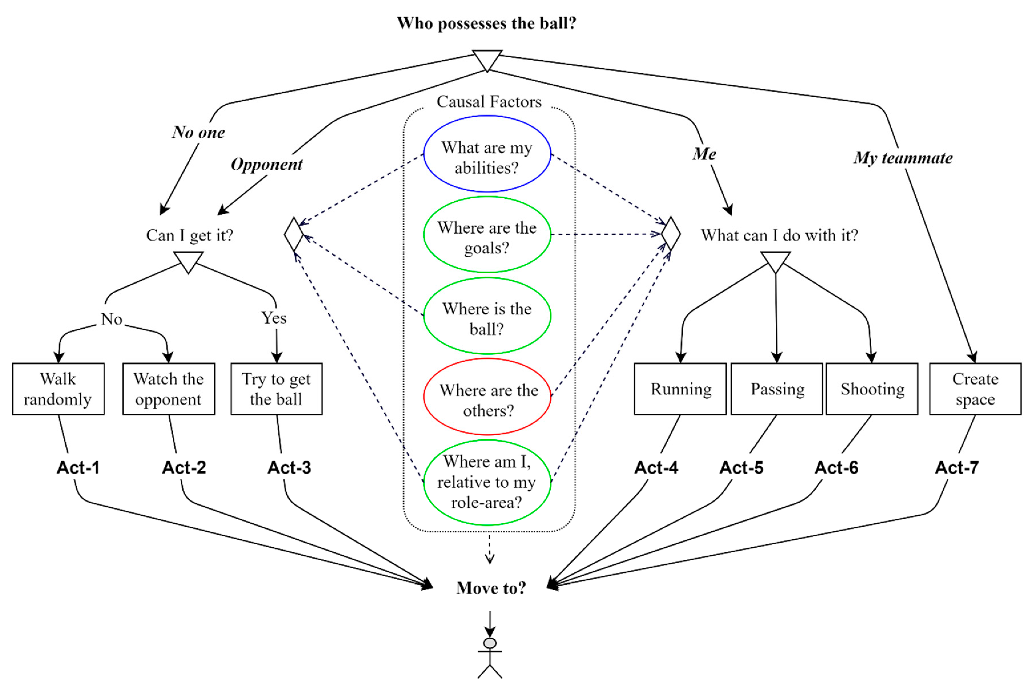
• The zero-order factors characterise the players’ inherent capabilities. These are ‘Stamina’, ‘Energy’, ‘Pace’, ‘Agility’, and ‘Shooting’ abilities (or attributes).
• The first-order causes represent the environmental actors. These actors include an imagined hard-bounded-box around each player’s role-area (an area that players mostly tend to move within), the elements that shape the football pitch (i.e., boundaries), and the Goals. The ball is also considered as an environmental actor, as it does not move due to an autonomously-made decision.
• The second-order causal factors indicate the interactions between this auto-agent and other auto-agents (players).

Figure 5. Autonomous agents (players) and environmental actors (player role-boxes, pitch, goals, ball) in the football simulation (zero-order capabilities not shown).

Figure 5. Autonomous agents (players) and environmental actors (player role-boxes, pitch, goals, ball) in the football simulation (zero-order capabilities not shown).

This configuration explicates three types of interaction: among auto-agents (e.g., a player and teammates), between auto-agents and environmental actors (e.g., players and the ball), among environmental actors (e.g., the ball and the pitch’s boundaries).

Figure 6 shows a simplified mechanism underlying the football players’ movement decision based on the above set of assumptions. An autonomous movement decision involves selecting a direction and speed (zero if not moving), based on player objectives of movement (actions). To select an action, players try to find out ‘who possesses the ball’ first and foremost. If it is possessed by an opponent, they find a location at which they can possibly intercept and possess the ball, dependent on their current abilities, ball velocity, and whether it is inside their role-area. Otherwise, they decide to closely move with the nearest opponent.

When players possess the ball, they choose either to carry or shoot the ball towards the opponent’s goal, or to pass it to one of their teammates, as a function of distance to opponents, to goals, to the centre of their role-box and their current abilities. If one of the player’s teammates possesses the ball, players try to create empty space or move randomly around the centre of their role-area. These actions are subject to player capability, e.g., current level of energy, which decreases throughout the game as a function of stamina.

In ABM, it is important to inspect model behaviours under various configurations to understand the potential mechanisms upon which the complex movement patterns emerge (see Figure 7 and Supplementary Materials). Given the complexity and variety of model outcomes, three types of outcome were focussed on in assessment: (i) ball possession patterns, (ii) the frequency of executed actions (objectives of movement: Act-1 to Act-7), and (iii) players’ movement relative to the ball and the closest opponent player. A total of five configurations of model parameters were used to generate outcomes, varying energy consumption (E), formation (F), and marking strategy (M):

• E—consumed, F—3-5-2, M—man-to-man (C1);
• E—not consumed, F—3-5-2, M—man-to-man (C2);
• E—consumed, F—3-5-2 (Team A) 4-4-3 (Team B), M—man-to-man (C3);
• E—consumed, F—4-4-3 (Team A) 3-5-2 (Team B), M—man-to-man (C4);
• E—consumed, F—3-5-2, M—zonal marking plan (C5).

Figure 7. Selection of result visualisations for team, role and individual aspects: (a) Changing ball possession among players and between teams for selected configurations. The green colour indicates successful passes among teammates. The red cells show the accumulated number of successful attempts to get the ball (retrieves, tackles, interceptions etc.) from the opposition; (b,c) The variation of selected executed actions (attempting ball possession, shooting, running into space) over all configurations, at individual-level. The lower values in Act-6 (the shooting case) are due to the requirement for possession of the ball, making it relatively rare; (d) Relative distance and orientation towards the ball for Player 10 only. Some values for the dominant ‘north’ orientation (i.e., towards the ball) beyond the plot extent are represented as numbers according to colour-coded configuration.

Figure 7. Selection of result visualisations for team, role and individual aspects: (a) Changing ball possession among players and between teams for selected configurations. The green colour indicates successful passes among teammates. The red cells show the accumulated number of successful attempts to get the ball (retrieves, tackles, interceptions etc.) from the opposition; (b,c) The variation of selected executed actions (attempting ball possession, shooting, running into space) over all configurations, at individual-level. The lower values in Act-6 (the shooting case) are due to the requirement for possession of the ball, making it relatively rare; (d) Relative distance and orientation towards the ball for Player 10 only. Some values for the dominant ‘north’ orientation (i.e., towards the ball) beyond the plot extent are represented as numbers according to colour-coded configuration.

For a single model run, Figure 7a shows intra- and inter-team ball possession patterns for most configurations. An example role-based pattern emerging is Team A’s strong link between midfielders and strikers and Team B’s emphasis on the defender-midfielder link, seemingly due to individual attributes (e.g., high average stamina). Figure 7b,c shows the frequency of selected executed actions over all configurations for each player (player numbers are in order of roles—goalkeeper, defender, midfielder, striker—for both teams), demonstrating a consistency from player to equivalent player in the opposing team (roles demonstrate consistent groupings, too). Figure 7d shows the movement and distance relative to the ball for one player only (Player 10, the most active agent). One obvious trend that emerges is that the closer the player is to the ball, the more consistently oriented towards the ball that player is.

Referring to the model parameters used to structure this model assessment, the variation of team formation has a bigger impact on the emergent outcome than the energy consumption rate and marking strategy, possibly due to the high influence of role-boxes on the running of the simulation. Ultimately, the movement behaviour of players does not seem to change radically across all the model settings, which underpins the robustness of the simulation.

6. Discussion

Movement analysis applications draw concepts and implement methods from CMA, GIScience, GeoComputation, ABM, and recently AI, which are neither necessarily compatible nor designed to pursue common objectives. Additionally, while the new generation of computational movement studies effectively advocates answering some ‘what’ and ‘what-if’ questions, conceptualization and implementation is needed for a model that can handle ‘how’ and ‘why’ inquiries. Such a model needs to theoretically comply with concepts from the diverse literature underpinning CMA and causal analysis, while remaining compatible with computational algorithms.

Theoretically, one data-driven and one simulation-based school of thought (GCM and ABM in practice) both claim to explore scientific causally relevant evidence. Although principally different, both approaches are founded on the idea that an initial model of a phenomenon is necessary for causal analysis. Counterfactual analysis is also central to both approaches: one investigates it by controlling for possible confounders and an intervention, while the other simply simulates alternative realities and observes them. In GCMs, causal analysis begins with making a model on what variables (events) might have caused a phenomenon, then setting one of them to a value to explore what would have happened if it had been different, and finally concluding why the phenomenon has happened. While in ABMs, causal mechanisms are pursued by encoding a set of assumptions in a model configuration, generating what would have happened under such configuration, and representing what chain of connections may have caused the phenomenon.

Whilst both methodologies are increasingly being developed and used in different fields, their utility for scientific understanding is the subject of many recent disagreements. ABMs are accused of being too simplistic or, at best, black-boxes that run under untestable assumptions. GCMs are criticised for being highly dependent on data, and incapable of dealing with complex mechanisms. They both also rely on theoretical, substantive, and domain-specific knowledge to show that the assumptions on which the causal identification strategy relies are satisfied.

A few solutions have been proposed across a range of different disciplines to address some of these challenges. For example, Herd and Miles [55] present an intervention-based causal analysis model to explicate the complex causal mechanism within an agent-based simulation. Their automated approach is capable of examining and detecting causal connection between any given pair of events at a particular instant of time in ABMs. Opposite to this methodology, integrating both approaches into data-driven ABMs is also receiving interest in sociology, economics, and sports analysis. In data-driven agent architectures, the modellers’ initial assumptions, agents’ behaviours, and the outcomes could be constructed and validated based on collected observations [108,109,110]. The value of such an approach is that it can represent the plausible implications of the separate elements together and so provide a better understanding of their effects in ways that might not have been expected from understanding each element separately [63]. Such models can also facilitate testing the causal claims: where researchers have observed probabilistic correlations among variables, or the outcomes of an experimental intervention, ABMs may help to determine which causal claims are consistent with these observations. Casini and Manzo [24] go beyond these utilities and argue that when such a well-calibrated and validated model is built the hypothesis on which the model is founded is rational; therefore, the simulated mechanisms may be treated as a replica of their real-world counterparts; when these justifications are in place, generated counterfactuals from intervention on such simulated mechanisms appear credible. Both approaches seem appealing, but a data-driven architecture appears to be more plausible in CMA, particularly when a sufficient amount of movement data is accessible.

Acknowledging the value, and possibility, of data-driven ABMs in movement studies, we argue that it becomes increasingly important to develop a common ground that can facilitate the communications between different paradigms as more integrated applications appear. Figure 3 presents a three-level cognitive framework for explaining movement mechanisms along association, intervention, and counterfactual lines. This is founded on a conceptual agent-based model in which the movement mechanisms could be represented through reconstructing the causal effects of moving entities’ indigenous attributes, environmental actors, and other autonomous agents’ actions. These causal factors are observed, analysed, and validated over space, time, or both space and time. By way of demonstration, the proposed conceptual model was implemented, in a limited sense, to realise an agent-based representation of the movement behaviour of football players in a robust simulation, deriving insights at team, role and individual level.

In trying to extend the boundaries of a conceptual model we need to consider three sets of descriptive, explanatory, and predictive goals that are sought with what, how, why, and what if questions. Thus, scientific explanations and counterfactual predictions need explicit modelling of causation, which itself requires manipulation of data and imagination alongside validation of possible outcomes. These map to the notions of intervention and counterfactual operations that together with association are modelled in a conceptual framework, the ladder of causation [18], and are featured in our model as a strategy for extending what CMA can do. We have presented a few empirical instances as the essence of adopting a theoretically and computationally supported model for CMA (Table 1, Table 2 and Table 3). A small subset out of many potential questions were expressed here, which ought to be addressed by an entity that is equipped with reasoning ability. These instances are neither jointly exclusive nor mutually exhaustive, yet, may ambitiously guide an artificial agent in transition from the observation to deeper layers of operation in the conceptual cube. These exemplars were provided at a generic level to preserve the generality of the framework. Each inquiry was accompanied with an example question from the conceptualised agent-based football simulation to make their applications clearer.

7. Conclusions

Current movement data have encouraged researchers to prioritize finding credible narratives that account for the observed movement behaviours. This together with a widely accepted model would potentially enable both theoretical and applied CMA to shift their objectives from describing ‘what happened’ towards explaining ‘how and why it happens’. A conceptual framework necessitates finding commonalities in a vast array of phenomena in which space, time and moving objects are important. In an attempt towards a model that supports both theory and application, we put forward three conceptually different zero-, first-, and second-order causal factors to be measured in three temporal, spatial, and spatiotemporal dimensions that are being processed through three (association, intervention, and counterfactual) operation levels. This supports unifying 27 possible operations in a conceptual cube as an arena where movement related inquiries and their relevant objectives takes place.

This paper intended to contribute to the theory of GIScience by conceptualising an integrated framework for causal reasoning in movement analysis, moving beyond the current pattern recognition and visualization emphasis of that discipline. Planning future research, with the inclusion of putting the proposed model into practice, suggests a proposed three-level study. The first step is to fully design, implement, and test a model development guideline (based on the agent-structure proposed in this paper) through which an agent-based movement model can acquire explanatory status. The start of this model development guideline is summarised in this paper, and needs to be expanded on in a separate study. The second step would be an attempt to adopt the main concepts around the graphical causal models in CMA. These concepts are not intuitive and are often hard to be made sense of, particularly in a field with no or limited background. Given the complexity within movement observations, analysing a real-world scenario with GCMs may not be a practical choice for this (specific) purpose. Therefore, we aim and suggest working on a set of simulated data to examine the machinery of intervention and counterfactual analysis in the context of movement causal studies. Finally, a separate practical study is required to thoroughly implement and verify the applications of the proposed data-driven agent-architecture. Thus, the last step is to implement a GCM as the cognitive structure of auto-agents that would imbue them with a human-like mental model in an explanatory agent-based movement model. This aligns with the call for developing model-based AI algorithms that are increasingly being encouraged. Implementing this integrated architecture (a GCM-informed agent) can rightly be identified as the next key challenge for agent-based movement modelling, benefitting the wide range of disciplines (cognitive science, geography, computer and data science, machine learning, ecology, sociology, economics, as well as GIScience and movement analysis itself) in which movement is important.

References

1. Harvey, D. Explanation in Geography; Edward Arnold: London, UK, 1969. [Google Scholar]
2. Gudmundsson, J.; Laube, P.; Wolle, T. Computational Movement Analysis. In Springer Handbook of Geographic Information; Springer: Berlin/Heidelberg, Germany, 2011; pp. 423–438. [Google Scholar] [CrossRef]
3. Long, J.A.; Nelson, T.A. A Review of Quantitative Methods for Movement Data. Int. J. Geogr. Inf. Sci. 2013, 27, 292–318. [Google Scholar] [CrossRef] [Green Version]
4. Demšar, U.; Buchin, K.; Cagnacci, F.; Safi, K.; Speckmann, B.; Van de Weghe, N.; Weiskopf, D.; Weibel, R. Analysis and Visualisation of Movement: An Interdisciplinary Review. Mov. Ecol. 2015, 3, 5. [Google Scholar] [CrossRef] [PubMed] [Green Version]
5. Yuan, M. Human Dynamics in Space and Time: A Brief History and a View Forward. Trans. GIS 2018, 22, 900–912. [Google Scholar] [CrossRef]
6. Andrienko, G.; Andrienko, N.; Budziak, G.; Dykes, J.; Fuchs, G.; von Landesberger, T.; Weber, H. Visual Analysis of Pressure in Football. Data Min. Knowl. Discov. 2017, 31, 1793–1839. [Google Scholar] [CrossRef]
7. Andrienko, G.; Andrienko, N.; Anzer, G.; Bauer, P.; Budziak, G.; Fuchs, G.; Hecker, D.; Weber, H.; Wrobel, S. Constructing Spaces and Times for Tactical Analysis in Football. IEEE Trans. Vis. Comput. Graph. 2019. [Google Scholar] [CrossRef] [Green Version]
8. Miller, H.J.; Goodchild, M.F. Data-Driven Geography. Geo. J. 2015, 80, 449–461. [Google Scholar] [CrossRef]
9. Graser, A.; Widhalm, P.; Dragaschnig, M. The M3 Massive Movement Model: A Distributed Incrementally Updatable Solution for Big Movement Data Exploration. Int. J. Geogr. Inf. Sci. 2020, 34, 2517–2540. [Google Scholar] [CrossRef]
10. Bleisch, S.; Duckham, M.; Galton, A.; Laube, P.; Lyon, J. Mining Candidate Causal Relationships in Movement Patterns. Int. J. Geogr. Inf. Sci. 2014, 28, 363–382. [Google Scholar] [CrossRef] [Green Version]
11. Dodge, S.; Gao, S.; Tomko, M.; Weibel, R. Progress in Computational Movement Analysis—Towards Movement Data Science. Int. J. Geogr. Inf. Sci. 2020, 34, 2395–2400. [Google Scholar] [CrossRef]
12. Laube, P. Computational Movement Analysis; Springer: Berlin, Germany, 2014. [Google Scholar]
13. Lucey, P.; Bialkowski, A.; Carr, P.; Foote, E.; Matthews, I. Characterizing Multi-Agent Team Behavior from Partial Team Tracings: Evidence from the English Premier League. In 26th AAAI Conference on Artificial Intelligence; Association for the Advancement of Artificial Intelligence: Toronto, ON, Canada, 2012; pp. 1387–1393. [Google Scholar]
14. Yue, Y.; Lucey, P.; Carr, P.; Bialkowski, A.; Matthews, I. Learning Fine-Grained Spatial Models for Dynamic Sports Play Prediction. In IEEE International Conference on Data Mining; IEEE: Shenzhen, China, 2014; pp. 670–679. [Google Scholar] [CrossRef] [Green Version]
15. Le, H.M.; Yue, Y.; Carr, P.; Lucey, P. Coordinated Multi-Agent Imitation Learning. In ICML 2017: 34th International Conference on Machine Learning; Journal of Machine Learning Research: Sydney, NSW, Australia, 2017; pp. 1995–2003. [Google Scholar]
16. Le, H.M.; Carr, P.; Yue, Y.; Lucey, P. Data-Driven Ghosting Using Deep Imitation Learning. In Proceedings of the MIT Sloan Sports Analytics Conference, Boston, MA, USA, 3–4 March 2017; p. 15. [Google Scholar]
17. Zheng, S.; Yue, Y.; Hobbs, J. Generating Long-Term Trajectories Using Deep Hierarchical Networks. In Advances in Neural Information Processing Systems; Lee, D.D., Sugiyama, M., Luxburg, U.V., Guyon, I., Garnett, R., Eds.; Curran Associates: New York, NY, USA, 2016; pp. 1543–1551. [Google Scholar]
18. Pearl, J.; Mackenzie, D. The Book of Why: The New Science of Cause and Effect, 1st ed.; Basic Books: New York, NY, USA, 2018. [Google Scholar]
19. Darwiche, A. Human-Level Intelligence or Animal-like Abilities? Commun. ACM 2018, 61, 56–67. [Google Scholar] [CrossRef] [Green Version]
20. Harland, K.; Crooks, A.T.; See, L.; Batty, M. Agent-Based Models of Geographical Systems; Springer Science & Business Media: Dordrecht, The Netherlands, 2012. [Google Scholar]
21. Heppenstall, A.; Crooks, A. Guest Editorial for Spatial Agent-Based Models: Current Practices and Future Trends. Geoinformatica 2019, 23, 163–167. [Google Scholar] [CrossRef] [Green Version]
22. O’Sullivan, D.; Millington, J.; Perry, G.; Wainwright, J. Agent-Based Models—Because They’re Worth It? In Agent-Based Models of Geographical Systems; Springer Netherlands: Dordrecht, The Netherlands, 2012; pp. 109–123. [Google Scholar] [CrossRef]
23. Bonabeau, E. Agent-Based Modeling: Methods and Techniques for Simulating Human Systems. Proc. Natl. Acad. Sci. USA 2002, 99 (Suppl. 3), 7280–7287. [Google Scholar] [CrossRef] [Green Version]
24. Casini, L.; Manzo, G. Agent-Based Models and Causality: A Methodological Appraisal; The IAS Working Paper Series; Linköping University Electronic Press: Linköping, Sweden, 2016; Volume 7. [Google Scholar]
25. Manson, S.; An, L.; Clarke, K.C.; Heppenstall, A.; Koch, J.; Krzyzanowski, B.; Morgan, F.; O’sullivan, D.; Runck, B.C.; Shook, E.; et al. Methodological Issues of Spatial Agent-Based Models. J. Artif. Soc. Soc. Simul. 2020, 23. [Google Scholar] [CrossRef]
26. Lozano, A.C.; Li, H.; Niculescu-Mizil, A.; Liu, Y.; Perlich, C.; Hosking, J.R.M.; Abe, N. Spatial-Temporal Causal Modeling for Climate Change Attribution. In Proceedings of the 15th ACM SIGKDD International Conference on Knowledge Discovery and Data Mining, Paris, France, 28 June–1 July 2009; pp. 587–595. [Google Scholar] [CrossRef] [Green Version]
27. Luo, Q.; Lu, W.; Cheng, W.; Valdes-Sosa, P.A.; Wen, X.; Ding, M.; Feng, J. Spatio-Temporal Granger Causality: A New Framework. Neuroimage 2013, 79, 241–263. [Google Scholar] [CrossRef] [PubMed] [Green Version]
28. Zhu, J.Y.; Sun, C.; Li, V.O.K. An Extended Spatio-Temporal Granger Causality Model for Air Quality Estimation with Heterogeneous Urban Big Data. IEEE Trans. Big Data 2017, 3, 307–319. [Google Scholar] [CrossRef]
29. Christiansen, R.; Baumann, M.; Kuemmerle, T.; Mahecha, M.D.; Peters, J. Towards Causal Inference for Spatio-Temporal Data: Conflict and Forest Loss in Colombia. arXiv 2020, arXiv:2005.08639. [Google Scholar]
30. Hume, D. An Enquiry Concerning Human Understanding. In Essays and Treatises on Several Subjects; Printed for Andrew Millar: London, UK, 1758; Volume 2, pp. 215–396. [Google Scholar] [CrossRef] [Green Version]
31. Hitchcock, C. Probabilistic Causation. Stanford Encyclopedia of Philosophy; Zalta, E.N., Ed.; Stanford University: Stanford, CA, USA, 2018. [Google Scholar]
32. Kleinberg, S.; Mishra, B. The Temporal Logic of Causal Structures. In Twenty-Fifth Conference on Uncertainty in Artificial Intelligence (UAI2009); AUAI Press: Montreal, QC, Canada, 2009; pp. 303–312. [Google Scholar]
33. Lewis, D. On the Plurality of Worlds; Blackwell: Oxford, UK, 1986. [Google Scholar] [CrossRef]
34. Lewis, D.K. Counterfactuals; Cambridge University Press (CUP): Cambridge, MA, USA, 1973. [Google Scholar]
35. Hall, N. Two Concepts of Causation. In Causation and Counterfactuals; Collins, J., Hall, N., Paul, L.A., Eds.; MIT Press: Cambridge, MA, USA, 2004; pp. 225–276. [Google Scholar]
36. Hall, N. Structural Equations and Causation. Philos. Stud. 2007, 132, 109–136. [Google Scholar] [CrossRef] [Green Version]
37. Heckman, J.J. The Scientific Model of Causality. Sociol. Methodol. 2005, 35, 1–97. [Google Scholar] [CrossRef]
38. Rubin, D.B. Estimating Causal Effects of Treatments in Randomized and Nonrandomized Studies. J. Educ. Psychol. 1974, 66, 688–701. [Google Scholar] [CrossRef] [Green Version]
39. Pearl, J. Causal Diagrams for Empirical Research. Biometrika 1995, 82, 669–688. [Google Scholar] [CrossRef]
40. Pearl, J. Bayesian Netwcrks: A Model Cf Self-Activated Memory for Evidential Reasoning. In Proceedings of the 7th Annual Conference of the Cognitive Science Society, Irvine, CA, USA, 15–17 August 1985; pp. 329–334. [Google Scholar]
41. Pearl, J. Probabilistic Reasoning in Intelligent Systems: Networks of Plausible Inference; Morgan Kaufmann Publishers INC: San Francisco, CA, USA, 1988. [Google Scholar]
42. Pearl, J. Causality, 2nd ed.; Cambridge University Press: Cambridge, UK, 2009. [Google Scholar] [CrossRef]
43. Pearl, J. Causality: Models, Reasoning, and Inference; Cambridge University Press: Cambridge, UK, 2000. [Google Scholar]
44. Imbens, G.W. Potential Outcome and Directed Acyclic Graph Approaches to Causality: Relevance for Empirical Practice in Economics. J. Econ. Lit. 2020, 58, 1129–1179. [Google Scholar] [CrossRef]
45. Greenland, S.; Pearl, J.; Robins, J.M. Causal Diagrams for Epidemiologic Research. Epidemiology 1999, 10, 37–48. [Google Scholar] [CrossRef]
46. Robins, J.M. Data, Design, and Background Knowledge in Etiologic Inference. Epidemiology 2011, 23, 313–320. [Google Scholar] [CrossRef] [PubMed] [Green Version]
47. Glymour, M.M.; Greenland, S. Causal Diagrams. In Modern Epidemiology; Rothman, K., Greenland, S., Eds.; Lippincott Williams & Wilkins Company: Philadelphia, PA, USA, 2008; pp. 183–209. [Google Scholar]
48. Glymour, C.; Zhang, K.; Spirtes, P. Review of Causal Discovery Methods Based on Graphical Models. Front. Genet. 2019, 10. [Google Scholar] [CrossRef] [Green Version]
49. Morgan, S.L.; Winship, C. Counterfactuals and Causal Inference: Methods and Principles for Social Research, 2nd ed.; Cambridge University Press: Cambridge, UK, 2015. [Google Scholar]
50. Hitchcock, C. Causal Models. In Stanford Encyclopedia of Philosophy; Stanford University: Stanford, CA, USA, 2018; p. 79. [Google Scholar]
51. Elwert, F. Graphical Causal Models. In Handbooks of Sociology and Social Research; Morgan, S.L., Ed.; Springer: Dordrecht, The Netherlands, 2013; pp. 245–273. [Google Scholar] [CrossRef]
52. Shpitser, I.; Pearl, J. Complete Identification Methods for the Causal Hierarchy. J. Mach. Learn. Res. 2008, 9, 1941–1979. [Google Scholar] [CrossRef]
53. Pearl, J. The Causal Foundations of Structural Equation Modeling. In Handbook of Structural Equation Modeling; Hoyle, R.H., Ed.; Guilford Press: New York, NY, USA, 2012. [Google Scholar]
54. Abdulkareem, S.A.; Mustafa, Y.T.; Augustijn, E.W.; Filatova, T. Bayesian Networks for Spatial Learning: A Workflow on Using Limited Survey Data for Intelligent Learning in Spatial Agent-Based Models. Geoinformatica 2019, 23, 243–268. [Google Scholar] [CrossRef] [Green Version]
55. Herd, B.C.; Miles, S. Detecting Causal Relationships in Simulation Models Using Intervention-Based Counterfactual Analysis. ACM Trans. Intell. Syst. Technol. 2019, 10. [Google Scholar] [CrossRef] [Green Version]
56. Gilbert, N. Models, Processes and Algorithms: Towards a Simulation Toolkit. In Tools and Techniques for Social Science Simulation; Suleiman, R., Troitzsch, K.G., Gilbert, N., Eds.; Physica-Verl: Heidelberg, Germany, 2000. [Google Scholar]
57. Arnold, K.F. Statistical and Simulation-Based Modelling Approaches for Causal Inference in Longitudinal Data: Integrating Counterfactual Thinking into Established Methods for Longitudinal Data Analysis; University of Leeds: Leeds, UK, 2020. [Google Scholar]
58. Lovelace, R.; Dumont, M. Spatial Microsimulation with R.; CRC Press: Boca Raton, FL, USA, 2016. [Google Scholar]
59. O’Sullivan, D.; Haklay, M. Agent-Based Models and Individualism: Is the World Agent-Based? Environ. Plan. A Econ. Sp. 2000, 32, 1409–1425. [Google Scholar] [CrossRef] [Green Version]
60. Macy, M.W.; Willer, R. From Factors to Actors: Computational Sociology and Agent-Based Modeling. Annu. Rev. Sociol. 2002, 28, 143–166. [Google Scholar] [CrossRef]
61. Schelling, T.C. Micromotives and Macrobehavior; W. W. Norton & Company: New York, NY, USA, 2006. [Google Scholar]
62. Humphreys, P. The Chances of Explanation: Causal Explanation in the Social, Medical, and Physical Sciences; Princeton University Press: Princeton, NJ, USA, 2014. [Google Scholar]
63. Diez Roux, A.V. Invited Commentary: The Virtual Epidemiologist—Promise and Peril. Am. J. Epidemiol. 2015, 181, 100–102. [Google Scholar] [CrossRef] [Green Version]
64. Reynolds, C.W. Flocks, Herds, and Schools: A Distributed Behavioral Model. Comput. Graph. (ACM) 1987, 21, 9–34. [Google Scholar] [CrossRef] [Green Version]
65. Tang, W.; Bennett, D.A. Agent-Based Modeling of Animal Movement: A Review. Geogr. Compass 2010, 4, 682–700. [Google Scholar] [CrossRef]
66. McLane, A.J.; Semeniuk, C.; McDermid, G.J.; Marceau, D.J. The Role of Agent-Based Models in Wildlife Ecology and Management. Ecol. Modell. 2011, 222, 1544–1556. [Google Scholar] [CrossRef]
67. Wallentin, G. Spatial Simulation: A Spatial Perspective on Individual-Based Ecology—A Review. Ecol. Modell. 2017, 350, 30–41. [Google Scholar] [CrossRef]
68. Grimm, V.; Railsback, S.F. Individual-Based Modeling and Ecology; Princeton University Press: Princeton, NJ, USA, 2005. [Google Scholar]
69. Parrott, L.; Kok, R. A Generic, Individual-Based Approach to Modelling Higher Trophic Levels in Simulation of Terrestrial Ecosystems. Ecol. Modell. 2002, 154, 151–178. [Google Scholar] [CrossRef]
70. Ahearn, S.C.; Smith, J.L.D.; Joshi, A.R.; Ding, J. TIGMOD: An Individual-Based Spatially Explicit Model for Simulating Tiger/Human Interaction in Multiple Use Forests. Ecol. Modell. 2001, 140, 81–97. [Google Scholar] [CrossRef]
71. Batty, M. Agent-Based Pedestrian Modeling. Environ. Plan. B Plan. Des. 2001, 28, 321–326. [Google Scholar] [CrossRef] [Green Version]
72. Klügl, F.; Rindsfüser, G. Large-Scale Agent-Based Pedestrian Simulation. In Multiagent System Technologies; Petta, P., Müller, J.P., Klusch, M., Georgeff, M., Eds.; Springer: Berlin/Heidelberg, Germany, 2007; pp. 145–156. [Google Scholar] [CrossRef]
73. Bazzani, A.; Capriotti, M.; Giorgini, B.; Melchiorre, G.; Rambaldi, S.; Servizi, G.; Turchetti, G. A Model for Asystematic Mobility in Urban Space. In The Dynamics of Complex Urban Systems; Albeverio, S., Andrey, D., Giordano, P., Vancheri, A., Eds.; Physica-Verlag HD: Heidelberg, Germany, 2008; pp. 59–73. [Google Scholar] [CrossRef]
74. Pluchino, A.; Garofalo, C.; Inturri, G.; Rapisarda, A.; Ignaccolo, M. Agent-Based Simulation of Pedestrian Behaviour in Closed Spaces: A Museum Case Study. J. Artif. Soc. Soc. Simul. 2013, 17, 14. [Google Scholar] [CrossRef] [Green Version]
75. Crooks, A.; Croitoru, A.; Lu, X.; Wise, S.; Irvine, J.; Stefanidis, A. Walk This Way: Improving Pedestrian Agent-Based Models through Scene Activity Analysis. ISPRS Int. J. Geo-Inf. 2015, 4, 1627–1656. [Google Scholar] [CrossRef] [Green Version]
76. Torrens, P.M. Moving Agent Pedestrians through Space and Time. Ann. Assoc. Am. Geogr. 2012, 102, 35–66. [Google Scholar] [CrossRef]
77. Haklay, M.; O’Sullivan, D.; Thurstain-Goodwin, M.; Schelhorn, T. “So Go Downtown”: Simulating Pedestrian Movement in Town Centres. Environ. Plan. B Plan. Des. 2001, 28, 343–359. [Google Scholar] [CrossRef] [Green Version]
78. Schelhorn, T.; O’Sullivan, D.; Haklay, M.; Thurstain-Goodwin, M. STREETS: An Agent-Based Pedestrian Model; Centre for Advanced Spatial Analysis UCL: London, UK, 2005. [Google Scholar]
79. Pizzitutti, F.; Pan, W.; Feingold, B.; Zaitchik, B.; Álvarez, C.A.; Mena, C.F. Out of the Net: An Agent-Based Model to Study Human Movements Influence on Local-Scale Malaria Transmission. PLoS ONE 2018, 13. [Google Scholar] [CrossRef] [PubMed] [Green Version]
80. O’Sullivan, D.; Gahegan, M.; Exeter, D.J.; Adams, B. Spatially Explicit Models for Exploring COVID-19 Lockdown Strategies. Trans. GIS 2020, 24, 967–1000. [Google Scholar] [CrossRef] [PubMed]
81. Banerjee, B.; Abukmail, A.; Kraemer, L. Advancing the Layered Approach to Agent-Based Crowd Simulation. In Proceedings of the 22nd Workshop on Principles of Advanced and Distributed Simulation, Roma, Italy, 3–6 June 2008; IEEE Computer Society: Washington, DC, USA, 2008; pp. 185–192. [Google Scholar] [CrossRef]
82. Szymanezyk, O.; Dickinson, P.; Duckett, T. Towards Agent-Based Crowd Simulation in Airports Using Games Technology. In Lecture Notes in Computer Science (Including Subseries Lecture Notes in Artificial Intelligence and Lecture Notes in Bioinformatics); Springer: Berlin/Heidelberg, Germany, 2011; Volume 6682 LNAI, pp. 524–533. [Google Scholar] [CrossRef] [Green Version]
83. Pelekis, N.; Theodoulidis, B.; Kopanakis, I.; Theodoridis, Y. Literature Review of Spatio-Temporal Database Models. Knowl. Eng. Rev. 2004, 19, 235–274. [Google Scholar] [CrossRef]
84. Epstein, J.M.; Axtell, R. Growing Artificial Societies: Social Science from the Bottom Up; Brookings Institution Press: Washington, DC, USA, 1996. [Google Scholar]
85. Wooldridge, M. Intelligent Agents. In Multiagent Systems; Gerhard Weiss, Ed.; MIT Press: Cambridge, MA, USA, 1999; pp. 3–40. [Google Scholar] [CrossRef]
86. Macal, C.M.; North, M.J. Tutorial on Agent-Based Modeling and Simulation. In Winter Simulation Conference; Kuhl, M.E., Steiger, N.M., Armstrong, B.F., Joines, J.A., Eds.; IEEE: Orlando, FL, USA, 2005; pp. 2–15. [Google Scholar] [CrossRef]
87. Torrens, P.M.; Benenson, I. Geographic Automata Systems. Int. J. Geogr. Inf. Sci. 2005, 19, 385–412. [Google Scholar] [CrossRef] [Green Version]
88. Yu, C.; Peuquet, D.J. A GeoAgent-based Framework for Knowledge-oriented Representation: Embracing Social Rules in GIS. Int. J. Geogr. Inf. Sci. 2009, 23, 923–960. [Google Scholar] [CrossRef]
89. Moore, A. Geographical Vector Agent-Based Simulation for Agricultural Land-Use Modelling. In Advanced Geosimulation Models; Marceau, D.J., Benenson, I., Eds.; Bentham Science Publisher: Sharjah, United Arab Emirates, 2011; pp. 30–48. [Google Scholar]
90. Luck, M.; d’Inverno, M. A Conceptual Framework for Agent Definition and Development. Comput. J. 2001, 44, 1–20. [Google Scholar] [CrossRef]
91. Erwig, M.; Güting, R.H.; Schneider, M.; Vazirgiannis, M. Spatio-Temporal Data Types: An Approach to Modeling and Querying Moving Objects in Databases. Geoinformatica 1999, 3, 269–296. [Google Scholar] [CrossRef]
92. Nathan, R.; Getz, W.M.; Revilla, E.; Holyoak, M.; Kadmon, R.; Saltz, D.; Smouse, P.E. A Movement Ecology Paradigm for Unifying Organismal Movement Research. Proc. Natl. Acad. Sci. USA 2008, 105, 19052–19059. [Google Scholar] [CrossRef] [PubMed] [Green Version]
93. Blachowicz, J. How Science Textbooks Treat Scientific Method: A Philosopher’s Perspective. Br. J. Philos. Sci. 2009, 60, 303–344. [Google Scholar] [CrossRef] [Green Version]
94. Blaikie, N.W.H. Analyzing Quantitative Data: From Description to Explanation; Sage Publications: Thousand Oaks, CA, USA, 2003. [Google Scholar]
95. Hernán, M.A.; Hsu, J.; Healy, B. A Second Chance to Get Causal Inference Right: A Classification of Data Science Tasks. Chance 2019, 32, 42–49. [Google Scholar] [CrossRef] [Green Version]
96. Turchin, P. Quantitative Analysis of Movement: Measuring and Modeling Population Redistribution in Animals and Plants; Sinauer Associates: Sunderland, MA, USA, 1998. [Google Scholar]
97. Sharif, M.; Alesheikh, A.A. Context-Aware Movement Analytics: Implications, Taxonomy, and Design Framework. Wiley Interdiscip. Rev. Data Min. Knowl. Discov. 2018, 8, e1233. [Google Scholar] [CrossRef]
98. Buchin, M.; Dodge, S.; Speckmann, B. Similarity of Trajectories Taking into Account Geographic Context. J. Spat. Inf. Sci. Number 2014, 9, 101–124. [Google Scholar] [CrossRef]
99. Edelhoff, H.; Signer, J.; Balkenhol, N. Path Segmentation for Beginners: An Overview of Current Methods for Detecting Changes in Animal Movement Patterns. Mov. Ecol. 2016, 4, 21. [Google Scholar] [CrossRef] [Green Version]
100. Laube, P. Progress in Movement Pattern Analysis. In Behaviour Monitoring and Interpretation—BMI: Smart Environments; Gottfried, B., Aghajan, H., Eds.; IOS Press: Amsterdam, The Netherlands, 2009; pp. 43–71. [Google Scholar] [CrossRef]
101. Dodge, S.; Weibel, R.; Lautenschütz, A.-K. Towards a Taxonomy of Movement Patterns. Inf. Vis. 2008, 7, 240–252. [Google Scholar] [CrossRef] [Green Version]
102. Toohey, K.; Duckham, M. Trajectory Similarity Measures. SIGSPATIAL Spec. 2015, 7, 43–50. [Google Scholar] [CrossRef]
103. Su, H.; Liu, S.; Zheng, B.; Zhou, X.; Zheng, K. A Survey of Trajectory Distance Measures and Performance Evaluation. VLDB J. 2020, 29, 3–32. [Google Scholar] [CrossRef]
104. Andrienko, N.; Andrienko, G.; Pelekis, N.; Spaccapietra, S. Basic Concepts of Movement Data. In Mobility, Data Mining and Privacy; Springer: Berlin/Heidelberg, Germany, 2008; pp. 15–38. [Google Scholar] [CrossRef]
105. Spaccapietra, S.; Parent, C.; Damiani, M.L.; de Macedo, J.A.; Porto, F.; Vangenot, C. A Conceptual View on Trajectories. Data Knowl. Eng. 2008, 65, 126–146. [Google Scholar] [CrossRef] [Green Version]
106. Rein, R.; Memmert, D. Big Data and Tactical Analysis in Elite Soccer: Future Challenges and Opportunities for Sports Science. Springerplus 2016, 5, 1–13. [Google Scholar] [CrossRef] [Green Version]
107. Sarmento, H.; Marcelino, R.; Anguera, M.T.; CampaniÇo, J.; Matos, N.; LeitÃo, J.C. Match Analysis in Football: A Systematic Review. J. Sports Sci. 2014, 32, 1831–1843. [Google Scholar] [CrossRef] [PubMed] [Green Version]
108. Boero, R.; Bravo, G.; Castellani, M.; Squazzoni, F. Why Bother with What Others Tell You? An Experimental Data-Driven Agent-Based Model. J. Artif. Soc. Soc. Simul. 2010, 13, 6. [Google Scholar] [CrossRef] [Green Version]
109. Chen, S.-H.; Venkatachalam, R. Agent-Based Modelling as a Foundation for Big Data. J. Econ. Methodol. 2017, 24, 362–383. [Google Scholar] [CrossRef] [Green Version]
110. Bell, D.; Mgbemena, C. Data-Driven Agent-Based Exploration of Customer Behavior. Simulation 2018, 94, 195–212. [Google Scholar] [CrossRef] [Green Version]
Figure 1. An illustrated classification of causal analysis methodologies. The target methodologies in this paper are shown in italics.
Ijgi 10 00190 g001
Figure 2. A causal graph example on the variable set V = C ,   E ,   B . Variable C and E are assumed to be the cause-and-effect variables, respectively. While B represents a set of confounder variables that need to be held fixed to analyse the causal relation between C and E .
Ijgi 10 00190 g002
Figure 3. The conceptual representation of enquiries that an intelligent agent could possibly ask and answer by considering its: state of attributes, interactions with the environmental actors, and relations with other autonomous agents over space and time, and to differing levels of causal analysis.
Ijgi 10 00190 g003
Figure 4. The key movement analysis concepts interpreted in causal language, mapped to the Figure 3 conceptual cube. Three sets of causes of movement operate at three different levels of abstraction: categorised as zero-order (intrinsic attributes), first-order (interaction with environmental actors), and second-order (interaction with other auto-agents) factors. This figure illustrates that movement studies could analyse the effect of each causal factor across various dimensions (spatial, temporal, spatiotemporal, and trajectory-based movement descriptors) and levels of operation (association, intervention, counterfactual).
Ijgi 10 00190 g004
Figure 6. Schematic representation of football players’ movement decision based on the proposed agent-structure in Figure 3. In total, three sets of causes of movement (zero-order, first-order, and second-order factors) are represented in blue, green, and red colour, respectively.
Ijgi 10 00190 g006