
A Trajectory Ensemble-Compression Algorithm Based on Finite Element Method


School of Science, Zhejiang Sci-Tech University, Hangzhou 310018, China
*
Author to whom correspondence should be addressed.
†
These authors contributed equally to this work.
ISPRS Int. J. Geo-Inf. 2021, 10(5), 334; https://0-doi-org.brum.beds.ac.uk/10.3390/ijgi10050334
Submission received: 16 March 2021
/
Revised: 17 April 2021
/
Accepted: 10 May 2021
/
Published: 14 May 2021
Abstract
:Trajectory compression is an efficient way of removing noise and preserving key features in location-based applications. This paper focuses on the dynamic compression of trajectory in memory, where the compression accuracy of trajectory changes dynamically with the different application scenarios. Existing methods can achieve this by adjusting the compression parameters. However, the relationship between the parameters and compression accuracy of most of these algorithms is considerably complex and varies with different trajectories, which makes it difficult to provide reasonable accuracy. We propose a novel trajectory compression algorithm that is based on the finite element method, in which the trajectory is taken as an elastomer to compress as a whole by elasticity theory, and trajectory compression can be thought of as deformation under stress. The compression accuracy can be determined by the stress size that is applied to the elastomer. When compared with the existing methods, the experimental results show that our method can provide more stable, data-independent compression accuracy under the given stress parameters, and with reasonable performance.
1. Introduction
In location-based applications [1], there is a considerable amount of positioning data from sensors of vehicles, ships, and mobile phones. Taking Zhejiang Province of China as an example, 68T vehicle trajectory data and 19T ship trajectory data are generated every year, which brings many difficulties to the storage, processing, and analysis. Raw trajectories contain a lot of noise, some of which are caused by the signal drift of the sensors and others are caused by the random movement of the moving object. The compression of the raw trajectory can eliminate noise, reduce storage occupation, and improve the efficiency of data queries and processing. In the task of spatiotemporal data mining, noise reduction is helpful in a spatiotemporal pattern search from the trajectory [2].
Different application scenarios have different requirements on the compression ratio and compression accuracy. A very high compression ratio can be achieved if the vehicle trajectory is compressed based on the road network and only the turning point is retained [3,4,5]. However, when we want to analyze the lane change of vehicles, we need to reduce the compression ratio and improve the accuracy. For the vessel trajectory, since there is no fixed road constraint, the compression accuracy changes dynamically according to the requirement [6,7,8,9]. Lower compression accuracies are needed for ocean channel analysis, medium accuracy for periodic analysis of vessel, and higher for short-term route prediction of single vessel. In the trajectory monitoring application, there are similar dynamic requirements for the display of trajectory. When the display scale is small, the trajectory with a low accuracy and high compression ratio should be displayed. If the map window is zoomed in, then the higher accuracy trajectory should be displayed with the window scale increasing.
Therefore, trajectories can no longer be compressed in a fixed way and stored in advance. We call this kind of compression method as dynamic compression, whose accuracy changes dynamically with the requirement.
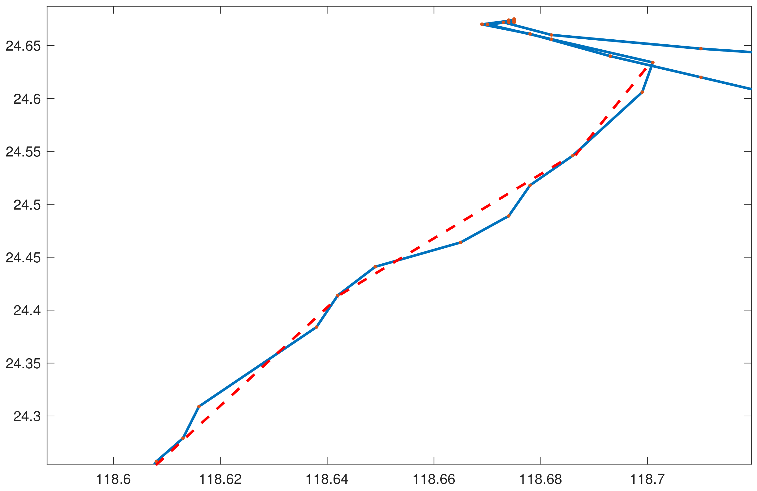
Trajectory compression tasks are traditionally divided into offline compression and online compression [10]. The former compresses all of the trajectories obtained, while the latter incrementally compresses the trajectories. In these methods, dynamic compression can be achieved by adjusting compression parameters. However, it is less certain what compression accuracy will result from a given compression parameter, and, even for different trajectories, the results will be different. Our study focuses on trajectory compression from another perspective—ensemble compression, is inspired by the human cognitive activity, which allows one to simplify trajectories without knowing the precise position of each point. People can draw simplified trajectories (the blue line is the raw trajectory, and the red one is the simplified trajectory) by intuitive feeling without accurate calculation of the exact position and distance, as shown in Figure 1. This is actually a compression method according to the whole features of the trajectory, and we call this kind of compression method ensemble compression. Inspired by this ensemble compression ability, we regard the trajectory as a physical entity, and trajectory compression can be thought of as deformation under uniform forces that are applied around the elastic object. The larger the deformation, the more points overlap due to mutual extrusion, so as to achieve the compression effect. In this research, we implement the trajectory ensemble compression algorithm that is based on finite element analysis, and in which we integrate the main direction of trajectory to achieve compression while preserving key features. The compression accuracy can be determined by the elastic parameters that are applied to the elastomer. When compared with the existing methods, the experimental results show that our method can provide more stable, data-independent compression accuracy under the given parameters, and with reasonable performance.
2. Related Work
Various trajectory compression algorithms are summarized by [10,11,12]. According to our research, the existing methods are divided into four categories: distance-based compression, gesture-based compression, map-constrained compression, and ensemble feature-based compression.
2.1. Distance-Based Compression
The distance-based compression algorithm analyzes each point in the trajectory in turn and decides whether to keep it or not according to its location, distance, direction, and other features of its adjacent points.
The Douglas–Peucker algorithm [13] is the first widely used trajectory compression algorithm. The algorithm connects the begin point and the end point of the original trajectory, and then calculates the distance from each point to the line. If the distance exceeds the threshold, then the trajectory is divided into two subsequences with the point as the splitting point, and then recursively performs the above process until the trajectory does not need to be divided. Another similar distance-based method is the Piecewise Linear Segmentation algorithm [14]. In this method, the point of most deviation is selected, and the threshold parameters are set to determine whether to retain the point, and the process executes recursively. In order to improve the efficiency of the distance-based algorithm, various algorithms have been made [15,16,17,18].
Another class of distance-based algorithms supports online compression. Two online algorithms are proposed by [15,19]: sliding window algorithm and open window algorithm, which build a sliding window on the point sequence, compress the trajectory in it, and then repeat the process for the subsequent trajectory data. Ref. [20] proposes the Dead Reckoning algorithm, which predicted the next point according to the points in the window and reserved points that greatly deviated from the forecast. Thye Dead Reckoning algorithm is improved by [21], who also proposed an algorithm, called Squish trajectory compression, which completes the compression by deleting the points with the least information loss in the buffered window. On the basis of these methods, many algorithms have been developed to further improve performance and reduce complexity [22,23,24,25,26].
2.2. Gesture-Based Compression
The distance-based compression method is greatly affected by different threshold parameters, and the improved method introduces gesture information to make up for the deficiency.
Ref. [27] proposes a trajectory compression method, which predicts the next point based on the speed and direction of historical data, and removes the predicted accurately points. The method is suitable for the high sampling density trajectories.
The stop points, similarity points, and turn points are also important semantic information that can be used in trajectory compression. For RFID location data [28], realize data compression by merging and closing the same location points of different trajectories [29], design a lossy compression strategy to collapse RFID tuples, which contain the information of items that are delivered in different locations.
Ref. [30] introduces the sampling information on the time series. Ref. [31] introduces the main direction of the trajectory to remove the noise. In [32], the speed information and stop point are introduced to improve the compression efficiency. The key points are preserved by [33] according to the velocity and direction data in the trajectory, and data compression is realized with these key points as constraints.
2.3. Map-Constrained Compression
Road information can improve the compression ratio. A large number of trajectory compression methods that are based on road constraints are proposed. A map-matching trajectory compression problem was first proposed by [4], where it is the combined problem of compressing trajectory at the same time matched on the underlying road network. The study gives a formal definition of the map matching compression problem, proposes two naive methods, and then designs improved online and offline algorithms. A path pruning simplification method is proposed by [34], which divides the trajectory simplification process into edge candidate set stage, path-finding stage, and path-refining stage. In the first stage, multiple candidate matching edges are obtained, In the second stage, road matching is performed with the assistance of driving direction for each trajectory position, In the third stage, the algorithm implements path tree pruning and it preserves the position in the trajectory where the direction changes. The algorithm runs on mobile device, which makes network transmission and central processing more efficient. The compressed points are selected by [5] according to the road network. Ref. [3] proposed a similar map matching system and implemented a track compression algorithm, called Heading Change Compression.
2.4. Ensemble Compression
Ensemble compression means that, when a trajectory is compressed, other geometric information that is related to the trajectory is combined, such as other similar trajectories, the boundary region of the trajectory, or the space-transformed trajectory.
When compared with the distance-based compression algorithm, there are few methods that are based on ensemble feature compression. Ref. [35] compress trajectories using convex hulls. The authors establish a virtual coordinate system with the starting point as the origin and the rectangular boundary around the trajectory, and make two boundary lines in each quadrant according to the direction of the trajectory. The rectangle and boundary lines form a convex hull, as well as the coordinate points in the constraint convex hull, are compressed.
Ref. [36] designs a trajectory similarity measurement method that is based on interpolation, in which the adopted method is similar to cluster. For each trajectory, the similar reference trajectory is found, and only the difference points with the reference one is retained, the similar points are removed.
In [37], a contour preserving algorithm for trajectory compression is proposed, which can compress the trajectory and keep the contour of the trajectory as much as possible. The algorithm divides the trajectory into multiple open windows, determines the main direction of each open window, and then compresses the trajectory points that deviate from the main direction.
Ref. [38] clusters all of the locations, match the clustering center on the road networks, and search the semantic events on the trajectory, such as parking, road switching, destination arrival, etc., to remove the random noise by only preserving semantic information points.
Ref. [39] regards the trajectories as time series, established linear equations of time and positions, and mapped the positions into the parameter space of the equations by hough transformation. Compression can be achieved by reducing three-dimensional data to hough space, in which the number of dual points is less than the number of points in the origin trajectory.
3. Trajectory Ensemble-Compression Algorithm
3.1. Preliminary
We give basic concepts related to the algorithm, in which Definitions 1 and 2 are the input of our algorithm, Definition 3 is the output of the algorithm, and Definitions 4–9 are the evaluation index.
Definition 1
(raw trajectory). The raw trajectory can be regarded as a sequence of locations () and attributes, as shown in (1). The attributes are only speed () and direction () of trajectory.
Definition 2
(main direction). A trajectory can be divided into several segments according to its driving direction. The main direction of vehicle is the direction of its road, while the main direction of vessel trajectory is fuzzy, different references have different definitions [6,7,8]. Our compression method makes no distinction between the vessels and vehicles, and the road network is not being used, so the main direction is obtained from only the raw trajectory. Its general definition is shown in (2).
is the ith point in the trajectory, length is the distance function, and direction is the azimuth function. According to Equation (2), the main direction of a segment that is composed of n points is the average of the directions of each part weighted by the length of each part.
Definition 3
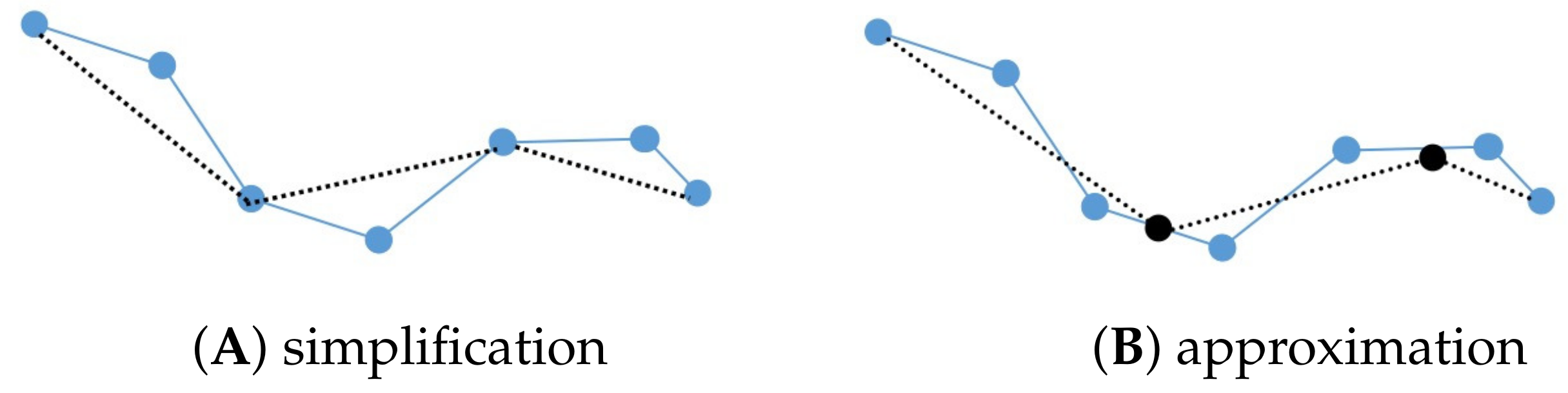
(simplification and approximation). There are two types of trajectory compression tasks, simplification and approximation. Simplification means that given a trajectory, a subsequence of the trajectory is generated, as shown in (Figure 2A). Approximation means generating a new sequence, as shown in (Figure 2B), where the two endpoints are the same.
Definition 4
(compression ratio). The ratio of the number of simplified trajectory points to the number of original trajectory points.
Definition 5
(the compression efficiency or compression rate). A point in the trajectory is composed of six double values: ID, longitude and latitude coordinates, speed, direction and time. Compression efficiency refers to the number of bytes that can be compressed per unit time.
Definition 6
(compression accuracy). The DTW algorithm [40] is used to calculate the trajectory distance before and after compression, which reflects the degree of their dissimilarity. The compression accuracy is defined as 1 minus this distance divided by the maximum DTW distance, which is the distance when the maximum compression occurs (only preserving the start and end points). The compression accuracy is between 0 and 1.
Definition 7
(compression error). compression error = 1 − compression accuracy.
Definition 8
(length ratio). The ratio of the sum of the lengths between two adjacent points the trajectory after simplification to the sum of the lengths between two adjacent points of the original trajectory.
Definition 9
(curvature ratio). curvature is the sum of the angles between segments, the curvature ratio is the angle sum after simplification to the angle sum of the original trajectory.
3.2. Algorithm Description
The input of the Ensemble-Compression algorithm includes the original trajectory and a set of elastic parameters, and the outputs either of the two compression results, although, in real applications, the focus is on simplification. The Algorithm 1 is shown in following.
| Algorithm 1 Ensemble-Compression |
|
Input: datas: trajectory sequence E: elastic modulus pro: poisson’s ratio density: mass density p: percentage maxit: maximum iterations tol: threshold rf: relaxation factor f: stress factor Output: sim: simplified trajectory appro: approximation range: mapping of points before and after simplification. //1.Intialization 1: ,, 2 //2.Discretization 3: 4: 5: //3.Element Analysis 6: 7: 8: //4.Semantic polymerization 9: 10: 11: 12: for i =1:length(pts) do 13: 14: 15: end for |
The algorithm consists of four modules. The initialization obtains the minimum boundary rectangle of the trajectory (line 1), and segments the trajectory (line 2), which is introduced in Section 3.4. The discretization realizes the interpolation and triangulation within the minimum boundary rectangle (lines 3–5), which is introduced in Section 3.2. The element analysis (lines 6–8) creates the stiffness matrix and stress matrix, and it solves the matrix equation to obtain the deformation trajectory. Section 3.3 introduces the matrix equation. Semantic polymerization (lines 9–15) deletes (trajectory simplification) or merges (trajectory approximation) the points too close to each other after deformation. In the deletion operation, selection is made according to the deviation from the main direction of the trajectory segment, and the points with large deviation are retained. Section 3.4 introduces semantic polymerization.
3.3. Discretization
The first step after initialization is to discretize the trajectory together with its bounding rectangle. We meshed the minimum boundary rectangle (line 3), merged mesh nodes and trajectory points (line 4), and then divided the elastomer into small units (line 5), as shown in Figure 3. We use delaunay triangulation [41] and the two-dimensional advancing front technique (AFT) [42] to complete the discretization.
3.4. Element Analysis
The main task of element analysis is to generate the element stiffness matrix and solve element matrix equation.
The element stiffness equation represents the relationship between the stress and triangular element, so that we can calculate the displacement of any point in the triangular element with a given magnitude and direction of the stress. For a single triangular element, Equation (3) shows the stiffness equation [41].
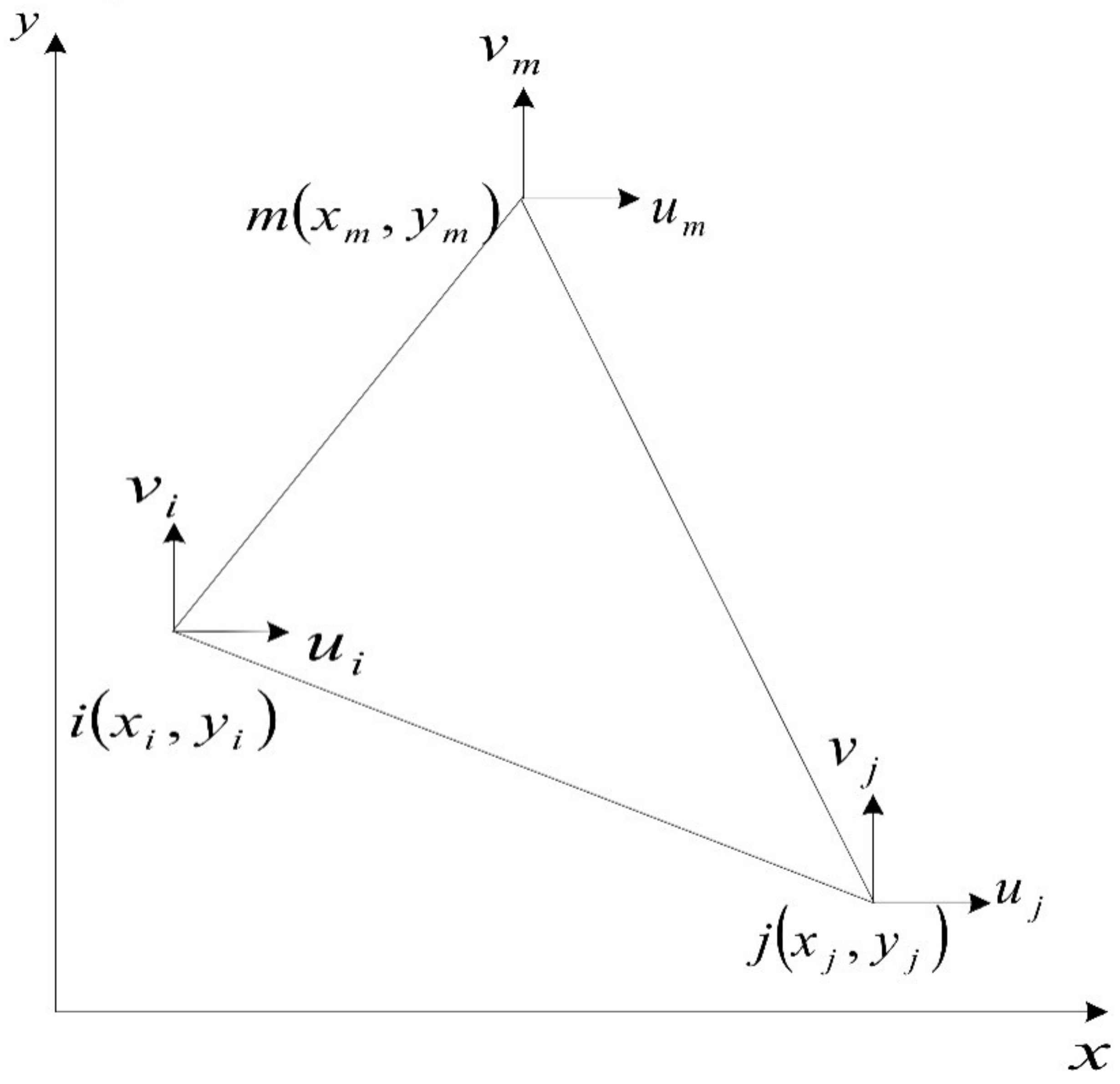
where t is the thickness of the element, is the elements area, and is the element displacement array, as shown in Equation (4). The three nodes of each triangular element (Figure 2) after triangulation are coded as i, j, and m. We take counterclockwise as the forward direction and establish the element displacement array.
is the stress column matrix of each node is shown in Equation (5).
D is the elastic matrix, as shown in Equation (6), in which E is the modulus of elasticity and u is Poisson’s ratio.
is the strain matrix of the element nodes, as defined in Equation (7) [41], in which are the stress coefficient constants.
Equation (4) gives the displacements of three nodes i,j, and m of the element under the stress, while the displacements of any point x and y in the triangular element can be obtained by solving Equations (8).
The six coefficients in the formula can be obtained by the positions and displacements of nodes i, j, and m.
The parentheses of Equation (3) are referred to stiffness matrix. The meaning of an element of the stiffness matrix is the stress to be applied to a node of the element, while the node has unit displacement and the others are zero.
Suppose that the whole is divided into m elements and n nodes, then the overall node displacement and the overall stress matrix F are all 2N× 1 matrix. Equation (9) shows the overall equilibrium equation of triangular element analysis:
3.5. Semantic Polymerization
The displacement of each point can be obtained using the above method. The stress causes spatial competition among the trajectory points. The simplified trajectories can be obtained by screening the subset of trajectories through the threshold, and the approximate trajectories can be obtained if the displacement of the subset is taken directly.
Based on the method shown in Section 3.4, the trajectory point displacement can be obtained (line 8). We calculate the distance at the adjacency point after displacement (line 9), normalize all the distances (line 9), and then sort all of the distances in ascending order. The points whose distance is less than the percentile threshold after sorting become candidate filter points (lines 10–11). Some points with key semantic information, such as direction or speed, will be deleted if only distance threshold is used, so we implemented a trajectory segmentation method based on the main direction. When two points compete due to the close distance, we keep those which are different from the main direction and stop points. The algorithm is shown in the following.
The input of Algorithm 2 is the trajectory sequence that is defined by Equation (1), in which each point is a five-dimensional array consisting of coordinates, time, speed, and direction. Algorithm 2 segments the trajectory according to the main direction of Equation (2). The algorithm adds four dimensions to the initial five dimensions. The sixth dimension records the length from the end of the last segment to the current point, which is the denominator of Equation (2). The seventh dimension records the product of the direction from the previous point to the current point and the sixth dimension, which is the numerator of Equation (2). The eighth dimension records the ratio of the seventh dimension to the sixth dimension, which is the main direction that is obtained by assuming the current point as the splitting point. The ninth dimension records the difference of the eighth dimension between the current point and previous point, which is, the deflection of the adjacent main direction. We take the position with the largest difference of main direction as the candidate splitting point. If the average of the main directions on both sides of the candidate point are very different, then the point is regarded as the end point of a new segment.
| Algorithm 2 Segmentation algorithm |
| Input: datas: trajectory sequence Output: segs: trajectory segments |
|
Algorithm 2 first initializes the values of the added four dimensions of the first point (lines 1–5). Subsequently, scan each point (line 6) and calculate the values of the four new dimensions of the current point (lines 7–9). Let t be the index of the maximum value of the 9th dimension, which is to find the position with the maximum deviation of the main direction (line 10), let d1 be the average of the main direction from the end of the previous segment to t (line 11), and d2 be the average of the main direction from t to the current point (line 12). If the difference between d1 and d2 is greater than the threshold, then t is regarded as the new segment end point (line 13). We record segments with array seg. For each segment, the starting point (line 14), the end position (lines 15–16), and the main direction of the segment are recorded in seg.
4. Experiment
4.1. Experimental Setup
We select GPS of taxi in Shanghai [44] and AIS of vessels crossing the East China Sea [7] as the experimental data. The taxi data set includes the 24-h trajectories of 4310 taxis, and the average sample frequency is 15 s. The vessel data set consisted of 120-h trajectories of 10,927 vessels with an average sample frequency of 10 s.
We compare our algorithm with two baselines [36,45], the former is offline compression algorithm (named OVTC), the latter is online compression algorithm(named SPM). In [36], many gesture information is considered in trajectory compression, such as static point, turn point, speed change point, break point, etc., so that the method has many compression parameters, and the optimal interval of these parameters is given. In [45], the sliding window, which is popular in the online compression, is improved, and the dynamic changing reference point is introduced to improve the compression efficiency. The sliding window size and threshold distance are the key parameters of the algorithm.
In the experiments, we fixed some parameters, including an elastic modulus of 2, Poisson’s ratio of 0.2, mass density of 1.15, maximum iteration number of 100, error threshold of 10 and relaxation factor of 1.
The percentiles of the experiment are 0.25, 0.35, 0.45, 0.55, 0.65, 0.75, 0.85, and 0.95, respectively. The external force factors (between 0–1) are 0.1, 0.2, 0.3, 0.4 0.5, 0.6, 0.7, 0.8, 0.9, and 1, and the direction of the force points to the center of gravity of the trajectory. The effects of different parameters on the compression indicators were observed. The experimental environment is Intel(R) Core(TM) i5 processor, 4 GB memory, Mac Darwin Kernel Version 17.7.0, and the development language is MatlabR2019.
4.2. Results
4.2.1. Comparative Study
The first concern is whether stable and data-independent compression accuracy can be obtained for a specific combination of parameters.
In OVTC, we fixed the parameter the distance threshold of the end stop point as 50 m, the speed threshold of the end stop point as 1.0 knots, and the gap threshold as 1800 s. The above values are the optimal values that are recommended by the reference through the evolutionary algorithm. We let three parameters change dynamically. The speed threshold at the start stop point is 0.05, 0.1, 0.25, 0.5, 0.75, 1.0, 1.25, 1.5, 1.75, and 2.0, the threshold of turn is 2.0, 10.0, 15.0, 20.0, and 25.0, and the threshold of speed change is 0.01, 0.2, 0.4, 0.6, and 0.8, resulting in 250 different compression parameters.
In SPM, we let two parameters change dynamically. According to the recommended range, we set the sliding window as 2, 5, 10, 15, and 20, and the distance threshold range as 5.0, 15.0, 25.0, 35.0, 45.0, 55.0, 65.0, 75.0, 85.0, 95.0, and 100.0, resulting in a total of 55 parameters.
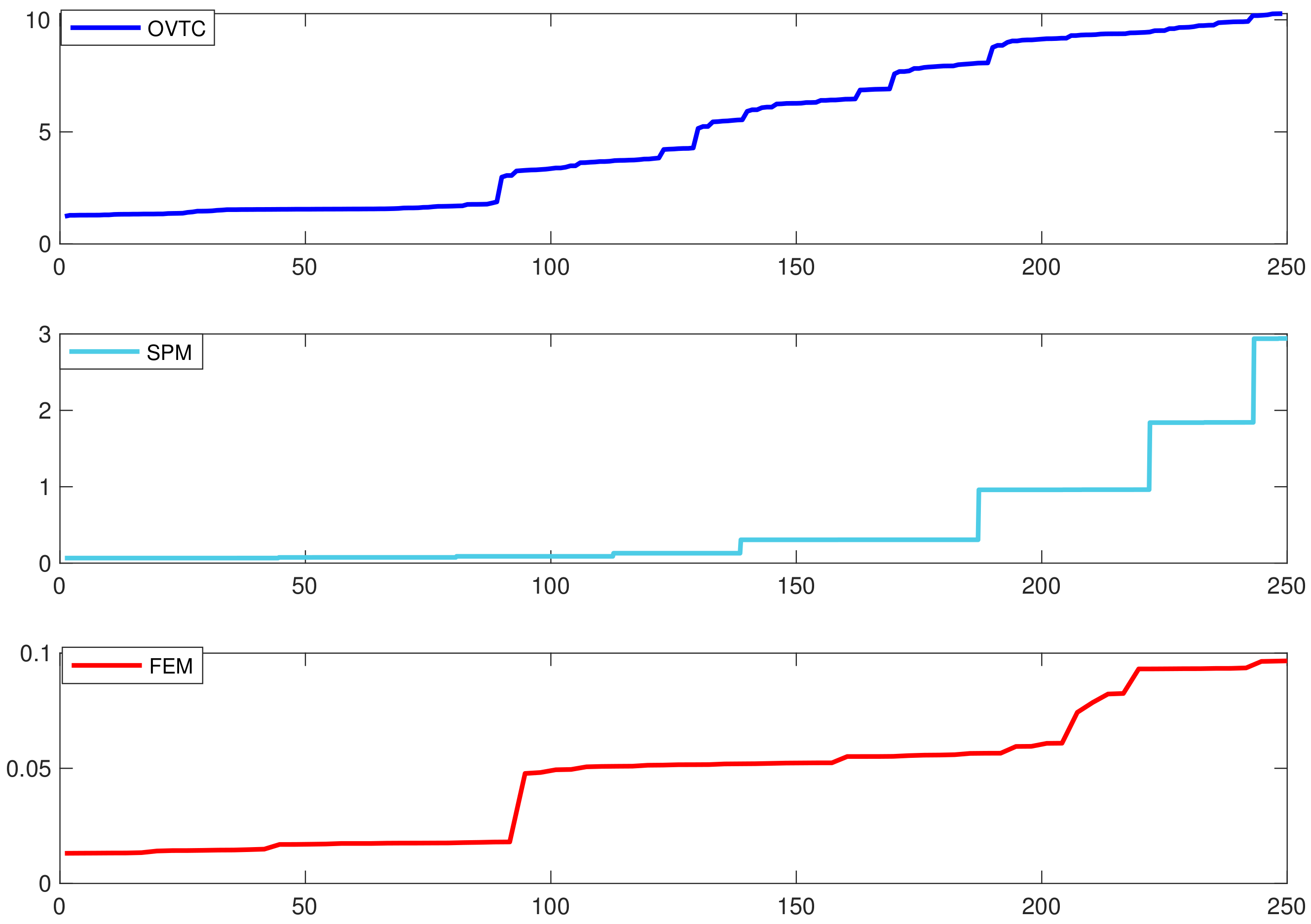
For each algorithm, all of the trajectories are compressed in each group of parameters. The standard deviations of compression accuracy obtained under different parameters and the std are displayed in ascending order, as shown in Figure 4.
In Figure 4, the horizontal axis is the number of 250 groups of parameters, and the vertical axis is the standard deviation of accuracy that is obtained by compressing all of the trajectories with corresponding parameters. The algorithm OVTC has the greatest uncertainty between compression parameters and accuracy, which may be due to the simultaneous use of direction, velocity, and distance thresholds. The algorithm SPM has both low standard deviation (left half) and high standard deviation (right half). The finite element method has a small standard deviation of accuracy under all parameters, which means that, when compared with the other two methods, it can get a certain accuracy under certain compression parameters. Although the standard deviation is different, the average accuracy of the three algorithms is very close, in which OVTC is 0.95159, SPM is 0.96056, and FEM is 0.943888.
Compression efficiency is another concern. We calculate the minimum, average, and maximum compression rates of the three algorithms under all parameters, as shown in Table 1.
Our method is smaller than the other two in the compression rate. The reason is that the finite element based method needs to solve the equations, while the other two methods only filter point-by-point. The average compression rate of FMT shown in Table 1 is 243.056 kbps, which can meet the needs of the real application scenarios described later (Section 4.2.5). The technology of concurrent services and cache in modern applications also make up for the deficiency of compression rate.
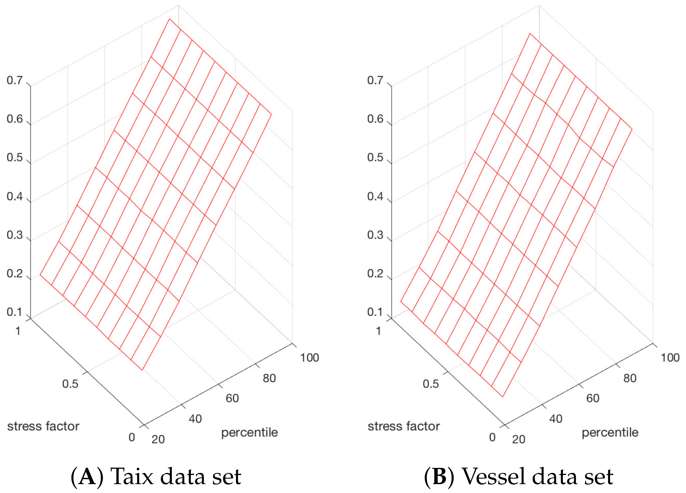
4.2.2. Influence of Percentile and Stress Factor on Compression Ratio and Compression Rate
The two data sets are compressed with different parameters, and Figure 5 shows the results.
Figure 5 shows that the compression ratio increases with the increase of the external force factor and with the decrease of the percentile. The influence of percentile on the compression rate is more obvious. When the stress factor remains unchanged, increasing the percentile can increase the compression ratio by 0.68.
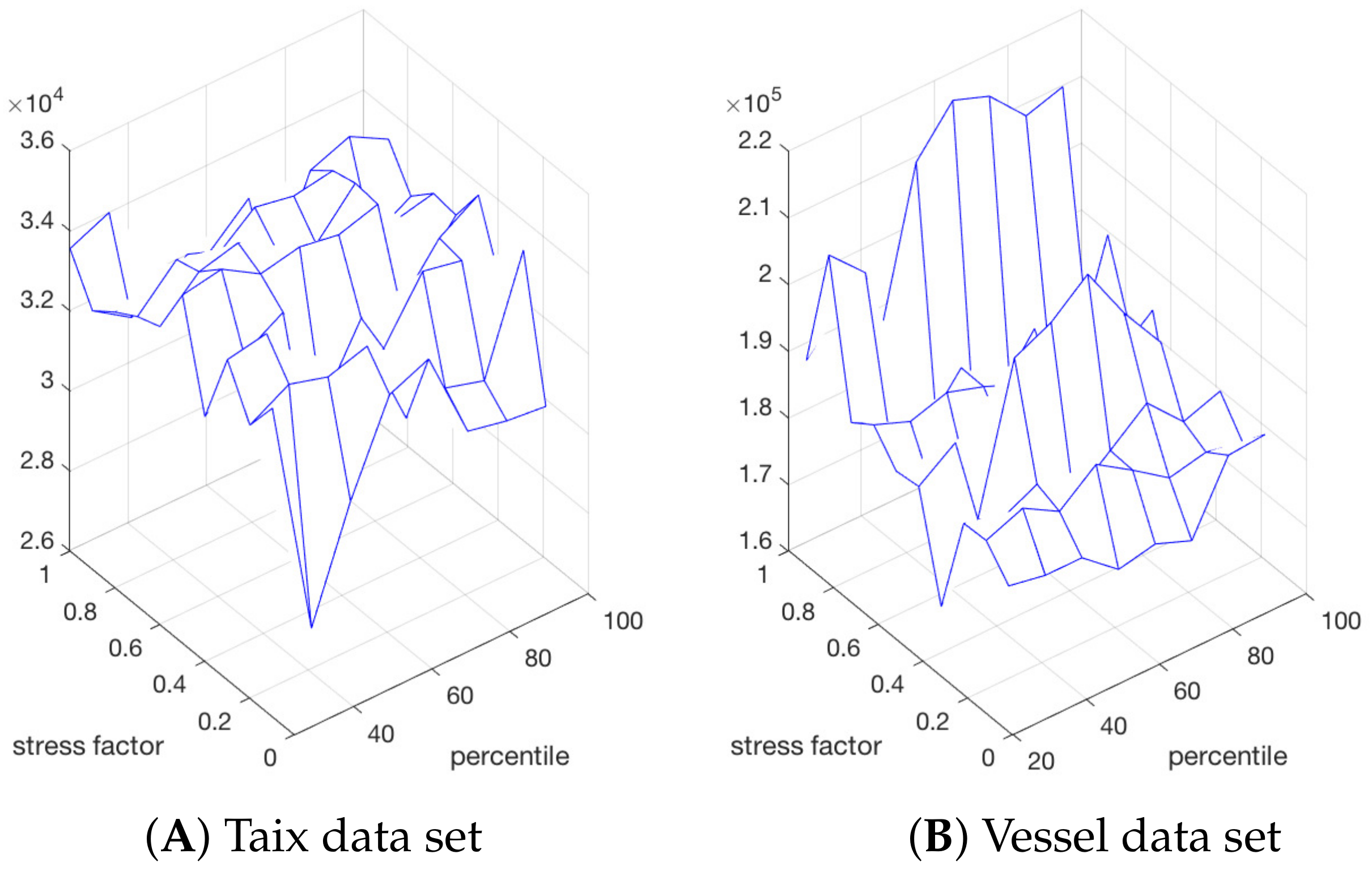
Figure 6 shows the effect of different parameters on the compression rate. Different from the compression ratio, the compression ratio is affected by both stress factor and percentile, and it is close to the maximum value when the stress factor value is 0.6.
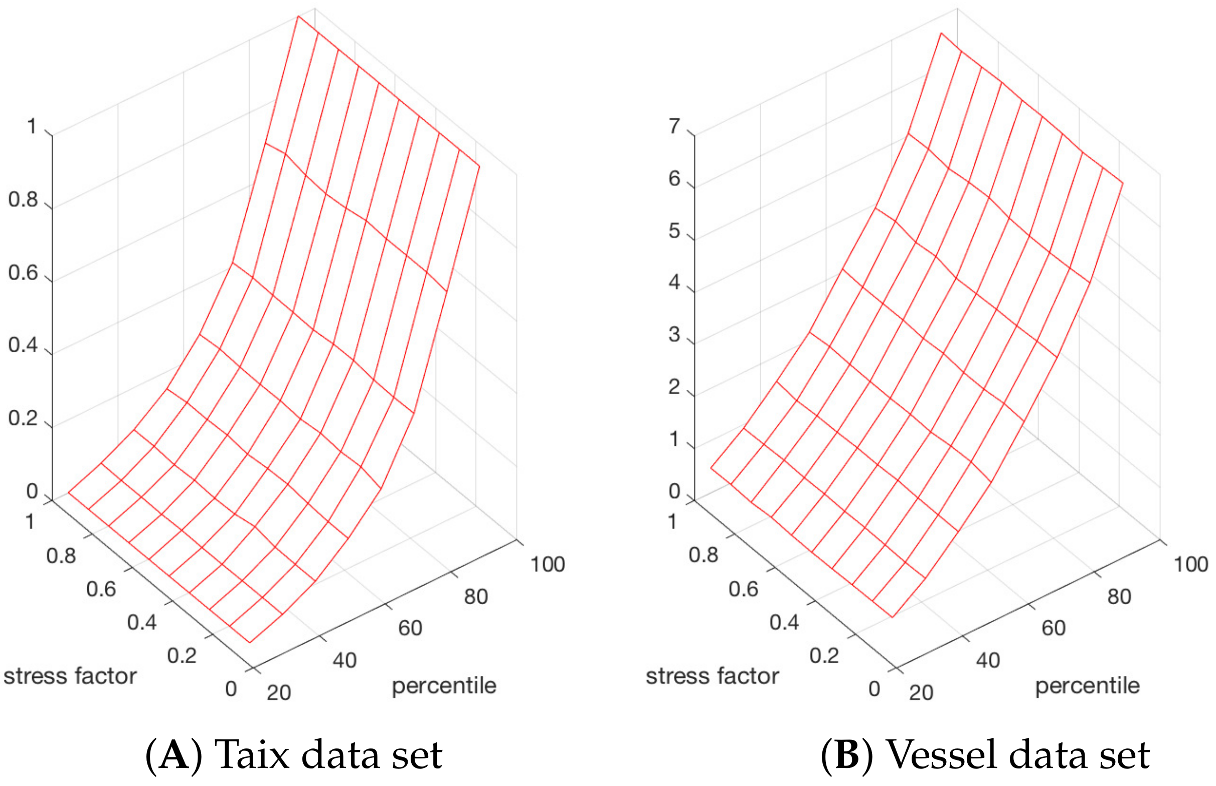
4.2.3. Compression Ratio and Compression Error
We use DTW algorithm [40] to calculate the distance of the trajectory before and after compression, which reflects the degree of compression error. The normalized distance can be considered as the relative error ratio that is caused by compression. The relative error ratio is the ratio of each DTW distance to the maximum DTW distance. The experiment shows the influence of various parameters on compression error, as shown in Figure 7.
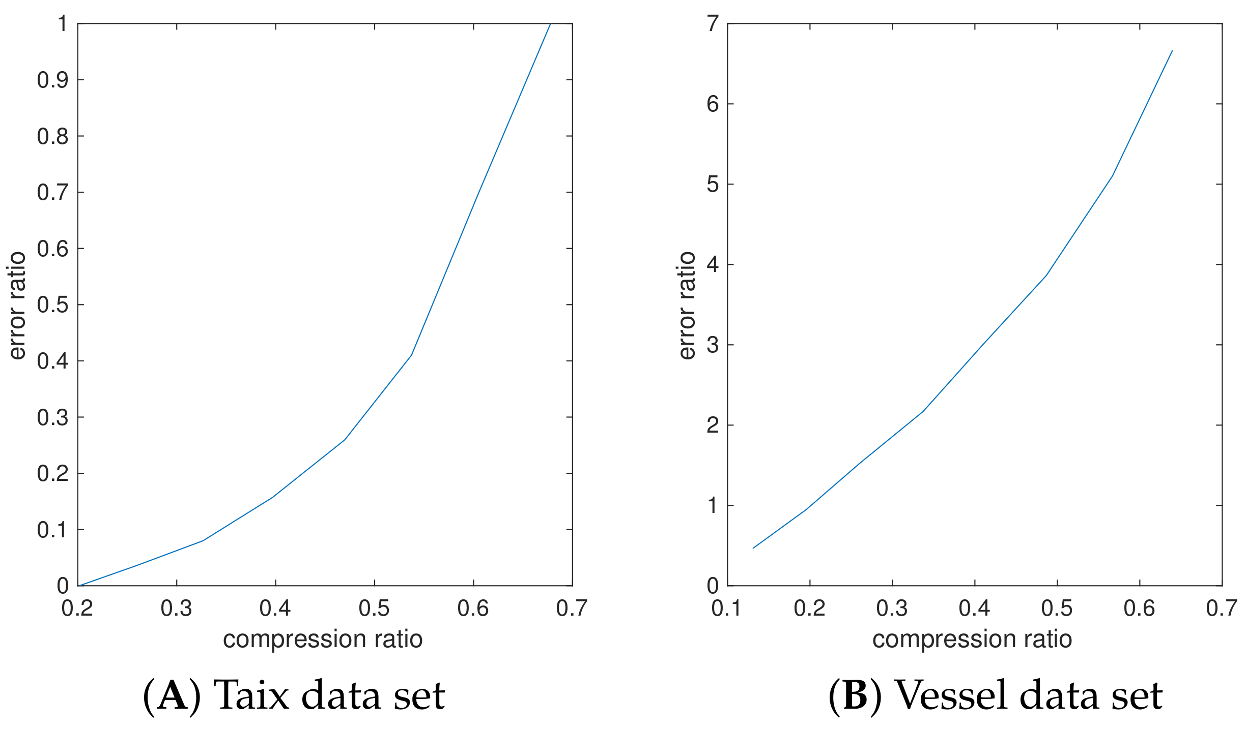
Figure 7 shows that the error ratio increases with the increase of percentiles. The relationship between the compression rate and error ratio was observed. The stress factor was fixed at 0.6 to observe the change of the error rate with the compression rate, as shown in Figure 8. For every 1% increase in the compression ratio, the error rate increases by 0.47%.
4.2.4. The Influence of Different Parameters on Other Indicators
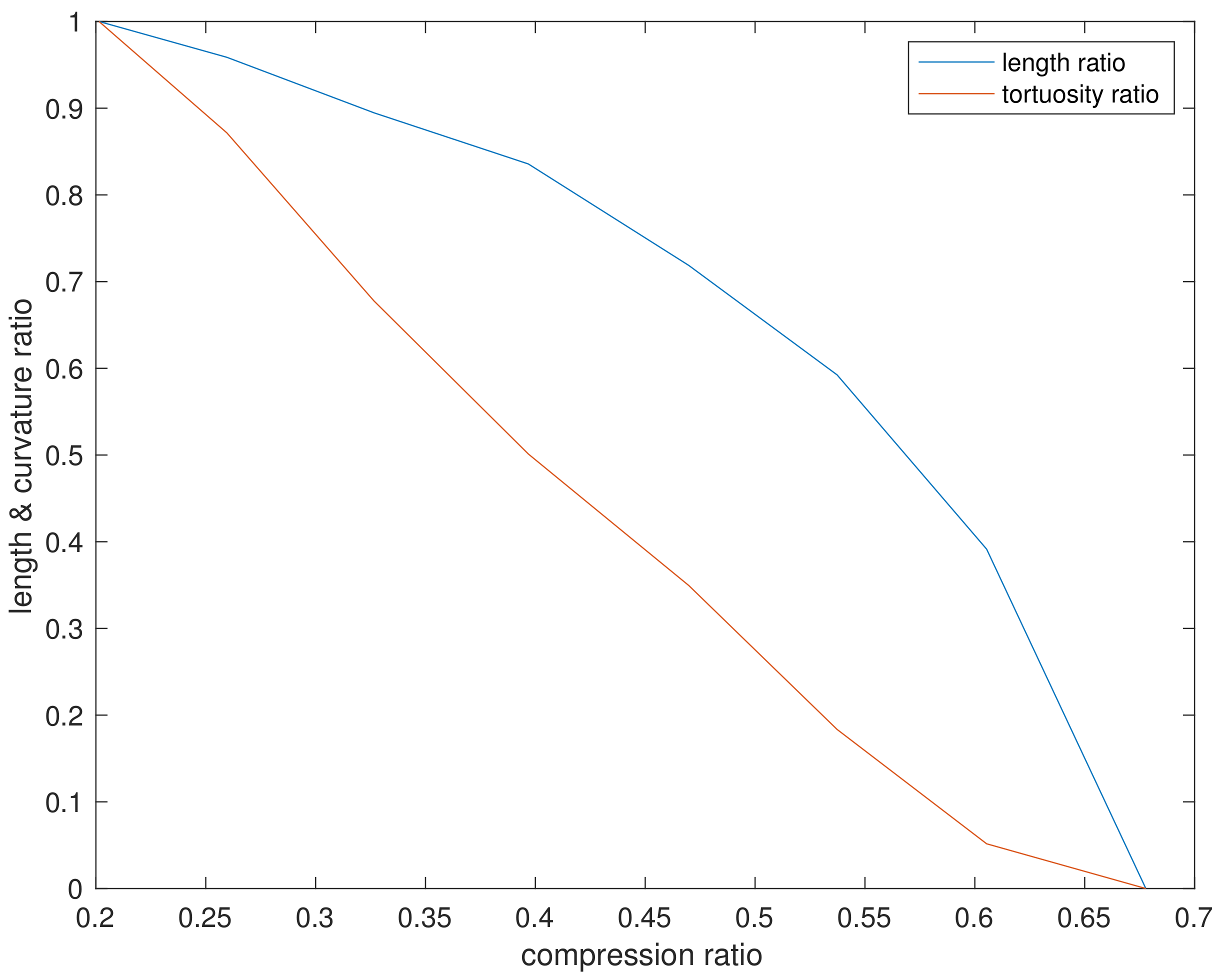
We study the effect of the algorithm on the length ratio and the curvature ratio. In the experiment, we fixed the stress factor as 0.6, and the results are shown in Figure 9.
As the compression ratio decreases, the length ratio and curvature ratio increase. Within the compression ratio of [20%, 40%], the length ratio and the curvature ratio are also maintained at a high level, which conforms to the geometric significance of the simplification [46]. It can also be seen that, even if the compression ratio is insignificant, the length ratio and the curvature ratio are maintained at a high level, and the distortion of the reaction curve is within a reasonable range.
4.2.5. Application Scenarios
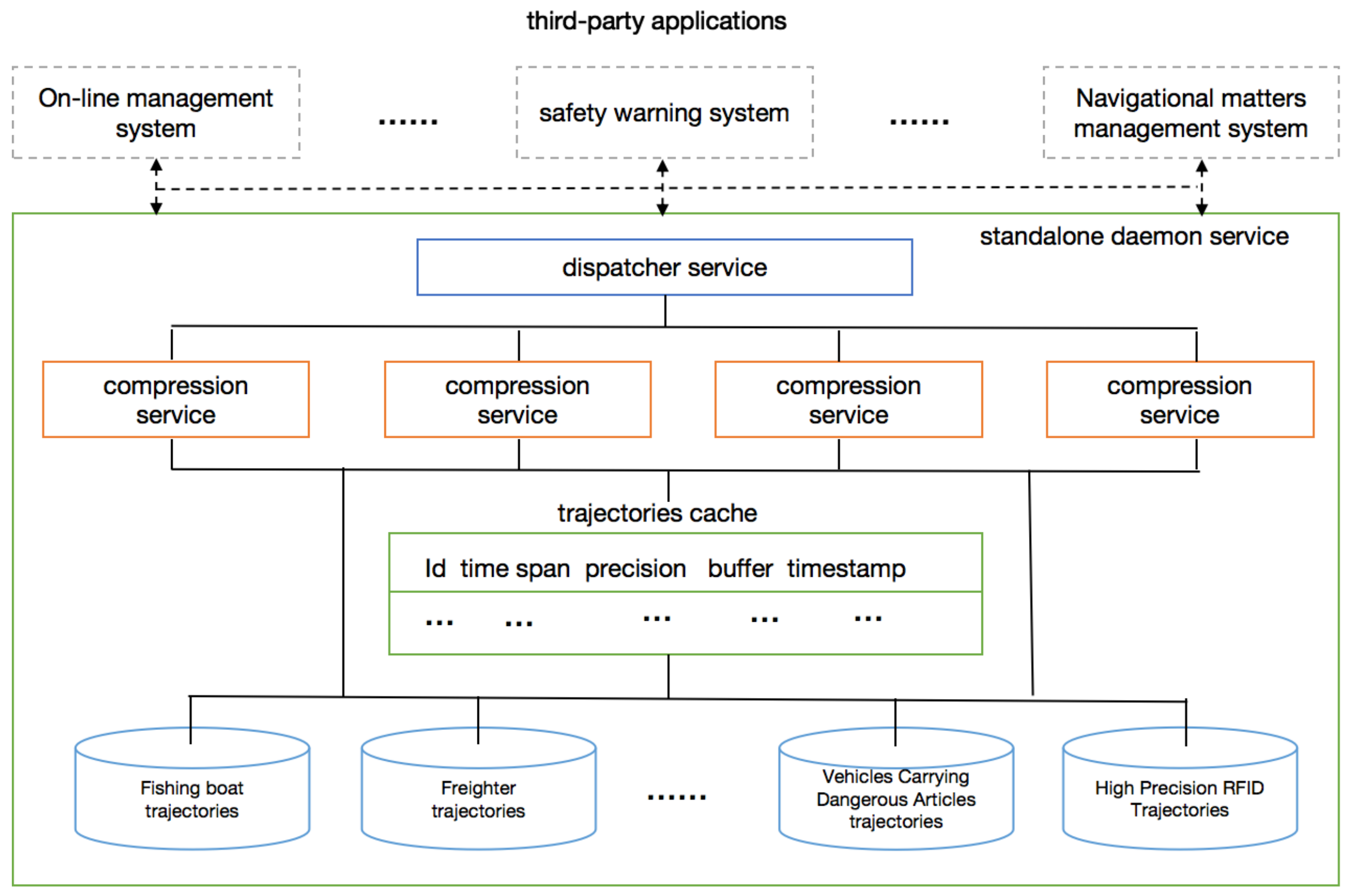
We develop an standalone daemon service, which is responsible for the management of multi-source spatial data, including vessel trajectory, vehicle trajectory, RFID, and it provides data query interfaces to multiple third-party applications. These third-party applications include online management systems, safety early warning systems, waterway management systems, etc. The data query service is required to be generic and application independent. Figure 10 shows the system overall.
The trajectory compression service is one of core in the system, which realizes concurrent processing and puts the compressed trajectory into the cache based on LRU for performance.
These applications submit the moving object id, time period, and trajectory precision (between 0–1), and the service returns the required trajectory. The precision here is interpreted as the accuracy of our method, which is, the compressed trajectory that is only composed of the begin and end point of the raw trajectory has the minimum accuracy, and the raw trajectory has the highest accuracy. Through the previous experiments, we can obtain the corresponding compression parameters for each accuracy interval, so that we can select the appropriate parameters to implement the compression process. Figure 11 shows example results of the same trajectory with different precision in different application. (A) is the trajectory with a compression ratio of 0.53 at a map scale of 1:200, (B) is the trajectory with a compression ratio of 0.26 at scale of 1:500 (zoomed to 1:200 to make it the same size as (A)). The larger the display scale, the smaller the compression ratio, and the more detail can be shown.
5. Discussion
Although the algorithm can meet the needs of above application, the algorithm also has some uncertain problems, the most important one is that it is actually a fuzzy compression strategy, and it does not accurately determine whether each point is noise. Therefore, it cannot be applied to the safety critical area without strict theoretical proof. Another problem is that it only considers the main direction, without speed and road network data. In the details of the implementation, the stress of each triangular element is the same, and the direction always points to the geometric center of the trajectory. It is not clear whether the result is different if the stress size and direction change with the point distribution density. All of these need to be further studied in the future.
6. Conclusions
In this work, a novel trajectory compression algorithm that is based on the finite element method is proposed, in which the trajectory is regarded as an elastomer that is deformed under external forces, and the trajectory is compressed with elasticity theory. The main direction segmentation algorithm is combined to achieve compression while preserving the key position information. The experiments show that our method can provide a more stable, data-independent compression ratio under the given stress parameters.
Accuracy is the only parameter selection basis of current compression algorithm, which is far from enough for rich practical applications. The ensemble compression algorithm that is based on finite element is only a preliminary attempt to realize dynamic compression service, and providing a customized trajectory, rather than fixed compression method should become an important research direction in related fields.
Author Contributions
Writing—draft, review and editing, Haibo Chen; software, Xin Chen. All authors have read and agreed to the published version of the manuscript.
Funding
This research received no external funding.
Institutional Review Board Statement
Not applicable.
Informed Consent Statement
Not applicable.
Data Availability Statement
https://github.com/bio-neuroevolution/ensemblecompression (accessed on 17 March 2021).
Conflicts of Interest
The authors declare no conflict of interest.
References
- Sadoun, B.; Al-Bayari, O. LBS and GIS Technology Combination and Applications. In Proceedings of the IEEE/ACS International Conference on Computer Systems & Applications, Amman, Jordan, 13–16 May 2007. [Google Scholar]
- Feng, Z.; Zhu, Y. A Survey on Trajectory Data Mining: Techniques and Applications. IEEE Access 2017, 4, 2056–2067. [Google Scholar] [CrossRef]
- Chen, C.; Ding, Y.; Xie, X.; Zhang, S.; Wang, Z.; Feng, L. TrajCompressor: An Online Map-matching-based Trajectory Compression Framework Leveraging Vehicle Heading Direction and Change. IEEE Trans. Intell. Transp. Syst. 2020, 21, 2012–2028. [Google Scholar] [CrossRef]
- Kellaris, G.; Pelekis, N.; Theodoridis, Y. Map-matched trajectory compression. J. Syst. Softw. 2013, 86, 1566–1579. [Google Scholar] [CrossRef]
- Zuo, Y.M.; Lin, X.L.; Shuai, M.A.; Jiang, J.H. Road Network Aware Online Trajectory Compression. J. Softw. 2018, 29, 734–755. [Google Scholar]
- Fikioris, G.; Patroumpas, K.; Artikis, A. Optimizing Vessel Trajectory Compression. In Proceedings of the 2020 21st IEEE International Conference on Mobile Data Management (MDM), Versailles, France, 30 June–3 July 2020; pp. 281–286. [Google Scholar] [CrossRef]
- Sheng, K.; Liu, Z.; Zhou, D.; He, A.; Feng, C. Research on Ship Classification Based on Trajectory Features. J. Navig. 2017, 71, 1–17. [Google Scholar] [CrossRef]
- Song, X.; Zhu, Z.L.; Gao, Y.P.; Chang, D.F. Vessel AIS Trajectory Online Compression Algorithm Combining Dynamic Thresholding and Global Optimization. Comput. Sci. 2019, 46, 333–338. [Google Scholar]
- Liu, J.; Li, H.; Yang, Z.; Wu, K.; Liu, Y.; Liu, R.W. Adaptive Douglas-Peucker Algorithm With Automatic Thresholding for AIS-Based Vessel Trajectory Compression. IEEE Access 2019, 7, 150677–150692. [Google Scholar] [CrossRef]
- Sun, P.; Xia, S.; Yuan, G.; Li, D. An Overview of Moving Object Trajectory Compression Algorithms. Math. Probl. Eng. Theory Methods Appl. 2016, 2016, 6587309.1. [Google Scholar] [CrossRef] [Green Version]
- Muckell, J.; Olsen, P.W.; Hwang, J.H.; Lawson, C.T.; Ravi, S.S. Compression of trajectory data: A comprehensive evaluation and new approach. Geoinformatica 2014, 18, 435–460. [Google Scholar] [CrossRef]
- Muckell, J.; Hwang, J.H.; Lawson, C.T.; Ravi, S.S. Algorithms for compressing GPS trajectory data: An empirical evaluation. ACM 2010. [Google Scholar] [CrossRef]
- Douglas, D.H.; Peucker, T.K. Algorithms for the Reduction of the number of points required to represent a digitized line or its caricature. Can. Cartogr. 2006, 10, 112–122. [Google Scholar] [CrossRef] [Green Version]
- Ding, Y.; Yang, X.; Kavs, A.J.; Li, J. A novel piecewise linear segmentation for time series. In Proceedings of the International Conference on Computer & Automation Engineering, Singapore, 26–28 February 2010. [Google Scholar]
- Meratnia, N.; By, R. Spatiotemporal Compression Techniques for Moving Point Objects. In Proceedings of the International Conference on Advances in Database Technology-Edbt, Heraklion, Greece, 14–18 March 2004. [Google Scholar]
- Brisaboa, N.R.; Gagie, T.; Gómezbrandón, A.; Navarro, G.; Paramá, J. Efficient Compression and Indexing of Trajectories; Springer: Cham, Switzerland, 2017. [Google Scholar]
- Lin, X.; Ma, S.; Zhang, H.; Wo, T.; Huai, J. One-Pass Error Bounded Trajectory Simplification. Proc. Vldb Endow. 2017, 10, 841–852. [Google Scholar] [CrossRef] [Green Version]
- Banerjee, P.; Ranu, S.; Raghavan, S. Inferring Uncertain Trajectories from Partial Observations. In Proceedings of the 2014 IEEE International Conference on Data Mining, Shenzhen, China, 14–17 December 2014. [Google Scholar]
- Keogh, E.; Chu, S.; Hart, D.; Pazzani, M. An Online Algorithm for Segmenting Time Series. In Proceedings of the 2001 IEEE International Conference on Data Mining, San Jose, CA, USA, 29 November–2 December 2002. [Google Scholar]
- Kolesnikov, A. Efficient Online Algorithms for the Polygonal Approximation of Trajectory Data. In Proceedings of the 12th IEEE International Conference on Mobile Data Management, MDM 2011, Luleå, Sweden, 6–9 June 2011; Volume 1. [Google Scholar]
- Deng, Z.; Wei, H.; Wang, L.; Ranjan, R.; Zomaya, A.Y.; Wei, J. An efficient online direction-preserving compression approach for trajectory streaming data. Future Gener. Comput. Syst. 2017, 68, 150–162. [Google Scholar] [CrossRef] [Green Version]
- Chen, M.; Xu, M.; FRnti, P. A Fast O(N) Multiresolution Polygonal Approximation Algorithm for GPS Trajectory Simplification. IEEE Trans. Image Process. 2012, 21, 2770–2785. [Google Scholar] [CrossRef] [PubMed]
- Liu, J.; Zhao, K.; Sommer, P.; Shang, S.; Kusy, B.; Lee, J.G.; Jurdak, R. A Novel Framework for Online Amnesic Trajectory Compression in Resource-Constrained Environments. IEEE Trans. Knowl. Data Eng. 2016, 28, 2827–2841. [Google Scholar] [CrossRef] [Green Version]
- Jia-Gao, W.U.; Liu, M.; Wei, G.; Liu, L.F. An Improved Trajectory Data Compression Algorithm of Sliding Window. Comput. Technol. Dev. 2015, 12, 47–51. [Google Scholar]
- Nibali, A.; He, Z. Trajic: An Effective Compression System for Trajectory Data. IEEE Trans. Knowl. Data Eng. 2015, 27, 3138–3151. [Google Scholar] [CrossRef]
- Gotsman, R.; Kanza, Y. A Dilution-matching-encoding compaction of trajectories over road networks. Geoinformatica 2015, 19, 331–364. [Google Scholar] [CrossRef]
- Zhang, D.; Ding, M.; Yang, D.; Yi, L.; Shen, H.T. Trajectory simplification: An experimental study and quality analysis. Proc. VLDB Endow. 2018, 11, 934–946. [Google Scholar] [CrossRef]
- Fazzinga, B.; Flesca, S.; Furfaro, F.; Masciari, E. RFID-data compression for supporting aggregate queries. ACM Trans. Database Syst. 2013, 38, 1–45. [Google Scholar] [CrossRef]
- Fazzinga, B.; Flesca, S.; Masciari, E.; Furfaro, F. Efficient and effective RFID data warehousing. In International Database Engineering and Applications Symposium (IDEAS 2009), 16–18, September 2009, Cetraro, Calabria, Italy; Desai, B.C., Sacc, D., Greco, S., Eds.; ACM International Conference Proceeding Series; Springer: Berlin/Heidelberg, Germany, 2009; pp. 251–258. [Google Scholar] [CrossRef]
- Long, C.; Wong, C.W.; Jagadish, H.V. Trajectory simplification: On minimizing the directionbased error. Proc. VLDB Endow. 2014, 8, 49–60. [Google Scholar] [CrossRef] [Green Version]
- Long, C.; Wong, C.W.; Jagadish, H.V. Direction-preserving trajectory simplification. Proc. VLDB Endow. 2013, 6, 949–960. [Google Scholar] [CrossRef] [Green Version]
- Ying, J.C.; Su, J.H. On Velocity-Preserving Trajectory Simplification. In Proceedings of the Asian Conference on Intelligent Information & Database Systems, Da Nang, Vietnam, 14–16 March 2016. [Google Scholar]
- Qian, H.; Lu, Y. Simplifying GPS Trajectory Data with Enhanced Spatial-Temporal Constraints. ISPRS Int. J. Geo-Inf. 2017, 6, 329. [Google Scholar] [CrossRef] [Green Version]
- Chen, C.; Ding, Y.; Wang, Z.; Zhao, J.; Guo, B.; Zhang, D. VTracer: When Online Vehicle Trajectory Compression Meets Mobile Edge Computing. IEEE Syst. J. 2020, 14, 1635–1646. [Google Scholar] [CrossRef] [Green Version]
- Liu, J.; Zhao, K.; Sommer, P.; Shang, S.; Kusy, B.; Jurdak, R. Bounded Quadrant System: Error-bounded Trajectory Compression on the Go. In Proceedings of the IEEE 31st International Conference on Data Engineering, Seoul, Korea, 13–16 April 2015. [Google Scholar]
- Birnbaum, J.; Meng, H.C.; Hwang, J.H.; Lawson, C. Similarity-Based Compression of GPS Trajectory Data. In Proceedings of the Fourth International Conference on Computing for Geospatial Research & Application, San Jose, CA, USA, 22–24 July 2013. [Google Scholar]
- Meng, Q.; Xiaoqiang, Y.U.; Liu, B.; Shao, L. A contour maintaining oriented trajectory data compression algorithm. J. Dalian Inst. Light Ind. 2018, 2, 139–145. [Google Scholar]
- Richter, K.F.; Schmid, F.; Laube, P. Semantic trajectory compression: Representing urban movement in a nutshell. J. Spat. Inf. Sci. 2012, 4, 3–30. [Google Scholar] [CrossRef]
- Dritsas, E.; Kanavos, A.; Trigka, M.; Sioutas, S.; Tsakalidis, A. Storage Efficient Trajectory Clustering and k-NN for Robust Privacy Preserving Spatio-Temporal Databases. Algorithms 2019, 12, 266. [Google Scholar] [CrossRef] [Green Version]
- Dtw, C. Information Retrieval for Music and Motion—Dynamic Time Warping; Springer: Berlin/Heidelberg, Germany, 2007. [Google Scholar]
- Mitchell, A.R. Finite Element Analysis and Applications; Cambridge University Press: Cambridge, UK, 2005. [Google Scholar]
- Jun-Ting, M.A.; Chen, S.Z.; Liu, H.; Zhang, J. Front Advancing Adaptive Triangular Mesh Generation Algorithm. Geogr. Geo-Inf. Sci. 2015, 31, 14–19. [Google Scholar]
- Bai, Z.Z. Modified Block SSOR Preconditioners for Symmetric Positive Definite Linear Systems. Ann. Oper. Res. 2001, 103, 263–282. [Google Scholar] [CrossRef]
- Ye, Y.; Sun, J.; Luo, J. Analyzing Spatio-Temporal Distribution Pattern and Correlation for Taxi and Metro Ridership in Shanghai. J. Shanghai Jiaotong Univ. (Sci.) 2019, 24, 137–147. [Google Scholar] [CrossRef]
- Sun, S.; Chen, Y.; Piao, Z.; Zhang, J. Vessel AIS Trajectory Online Compression based on scan-pick-move Algorithm added Sliding Window. IEEE Access 2020, 8, 109350–109359. [Google Scholar] [CrossRef]
- Zhai, J.; Li, Z.; Wu, F.; Xie, H.; Bo, Z. Quality Assessment Method for Linear Feature Simplification Based on Multi-Scale Spatial Uncertainty. ISPRS Int. J. Geo Inf. 2017, 6, 184. [Google Scholar] [CrossRef] [Green Version]
Figure 1.
Simplified trajectory by intuitive feeling.

Figure 2.
Two types of trajectory compression tasks

Figure 3.
Triangular element.

Figure 4.
Standard deviations of compression accuracy.

Figure 5.
Compression ratio at different parameters.

Figure 6.
Compression rate at different parameters.

Figure 7.
Error ratio at different parameters.

Figure 8.
Correlation between error ratio and compression ratio.

Figure 9.
The correlation between length ratio, curvature ratio, and compression ratio.

Figure 10.
Application System Overview.

Figure 11.
Compressed trajectoy in two applications.


Table 1.
Compression rates.
| Algorithm | Minimum | Average | Maximum |
|---|---|---|---|
| OVTC | 1547.65 Kbps | 8331.35 Kbps | 73,288 Kbps |
| SPM | 485.76 Kbps | 13,775.96 Kbps | 334,872.0 Kbps |
| FMT | 35.339 Kbps | 243.056 Kbps | 267.174 Kbps |
Publisher’s Note: MDPI stays neutral with regard to jurisdictional claims in published maps and institutional affiliations. |
© 2021 by the authors. Licensee MDPI, Basel, Switzerland. This article is an open access article distributed under the terms and conditions of the Creative Commons Attribution (CC BY) license (https://creativecommons.org/licenses/by/4.0/).
Share and Cite
MDPI and ACS Style
Chen, H.; Chen, X. A Trajectory Ensemble-Compression Algorithm Based on Finite Element Method. ISPRS Int. J. Geo-Inf. 2021, 10, 334. https://0-doi-org.brum.beds.ac.uk/10.3390/ijgi10050334
AMA Style
Chen H, Chen X. A Trajectory Ensemble-Compression Algorithm Based on Finite Element Method. ISPRS International Journal of Geo-Information. 2021; 10(5):334. https://0-doi-org.brum.beds.ac.uk/10.3390/ijgi10050334
Chicago/Turabian StyleChen, Haibo, and Xin Chen. 2021. "A Trajectory Ensemble-Compression Algorithm Based on Finite Element Method" ISPRS International Journal of Geo-Information 10, no. 5: 334. https://0-doi-org.brum.beds.ac.uk/10.3390/ijgi10050334
Note that from the first issue of 2016, this journal uses article numbers instead of page numbers. See further details here.