
Fine Crop Classification Based on UAV Hyperspectral Images and Random Forest

1
College of Geomatics and Geoinformation, Guilin University of Technology, Guilin 541006, China
2
School of Surveying and Geo-Informatics, Shandong Jianzhu University, Jinan 250101, China
3
School of Geographic Sciences, East China Normal University, Shanghai 200241, China
*
Author to whom correspondence should be addressed.
ISPRS Int. J. Geo-Inf. 2022, 11(4), 252; https://0-doi-org.brum.beds.ac.uk/10.3390/ijgi11040252
Submission received: 24 February 2022
/
Revised: 1 April 2022
/
Accepted: 7 April 2022
/
Published: 12 April 2022
(This article belongs to the Special Issue Integrating GIS and Remote Sensing in Soil Mapping and Modeling)
Abstract
:The classification of unmanned aerial vehicle hyperspectral images is of great significance in agricultural monitoring. This paper studied a fine classification method for crops based on feature transform combined with random forest (RF). Aiming at the problem of a large number of spectra and a large amount of calculation, three feature transform methods for dimensionality reduction, minimum noise fraction (MNF), independent component analysis (ICA), and principal component analysis (PCA), were studied. Then, RF was used to finely classify a variety of crops in hyperspectral images. The results showed: (1) The MNF–RF combination was the best ideal classification combination in this study. The best classification accuracies of the MNF–RF random sample set in the Longkou and Honghu areas were 97.18% and 80.43%, respectively; compared with the original image, the RF classification accuracy was improved by 6.43% and 8.81%, respectively. (2) For this study, the overall classification accuracy of RF in the two regions was positively correlated with the number of random sample points. (3) The image after feature transform was less affected by the number of sample points than the original image. The MNF transform curve of the overall RF classification accuracy in the two regions varied with the number of random sample points but was the smoothest and least affected by the number of sample points, followed by the PCA transform and ICA transform curves. The overall classification accuracies of MNF–RF in the Longkou and Honghu areas did not exceed 0.50% and 3.25%, respectively, with the fluctuation of the number of sample points. This research can provide reference for the fine classification of crops based on UAV-borne hyperspectral images.
1. Introduction
The classification of crops supported by remote sensing technology is one of the core means of realizing the promotion of agricultural development [1]. Compared with spaceborne and manned aviation hyperspectral systems, the UAV-borne hyperspectral remote sensing system can simultaneously obtain remote sensing images with nanometer-level hyperspectral resolution and centimeter-level high spatial resolution, which is more suitable for the current situation of the Chinese agricultural structure [2,3,4,5]. The continuous development of hyperspectral remote sensing technology has promoted the development of agricultural science and technology [6]. UAV hyperspectral imagery has a wide range of applications in crop yield estimation, single species classification, and disease monitoring, but many studies have focused on hyperspectral images of low spatial resolution [7,8,9,10].
To date, a classification algorithm based on deep learning has been used to classify crops [11,12], but the deep learning method has high requirements on the number of samples. Under the conditions of a small image area and a small number of samples, the application of the deep learning method in the fine classification of crops is limited to a certain extent [13]. Compared with deep learning algorithms, random forests have the characteristics of high efficiency, fewer samples required, and high classification accuracy, and their applications in environmental monitoring, land use, etc. have achieved impressive results [14,15,16,17]. Hongyan Yang et al. used the random forest classification algorithm to classify crops. The obtained classification accuracy was high, but the research categories were few, so it was difficult to determine the performance of the random forest classification algorithm in the case of more complex categories and feature information [18].
Hyperspectral images have many bands and a large amount of data, and large information redundancy affects the efficiency of classification operations [19,20]. Redundant bands also have an impact on classification accuracy when the number of classification samples is small [13]. Therefore, dimensionality reduction aiming at the problems of a large number of spectra and the large amount of calculation using feature transform is very important. Zahra Dabiri et al. systematically performed a comparison of independent component analysis (ICA), principal component analysis (PCA), and minimum noise fraction transformation (MNF) for classification of six tree species using APEX hyperspectral imagery [21]. However, there have yet been few targeted studies on the classification of various crops by different transforms.
Therefore, this study used high-spatial resolution hyperspectral image data from a UAV and adopted three dimensionality reduction transformation methods, MNF, ICA, and PCA. The random forest (RF) classification algorithm was then used to classify all kinds of crops in Honghu City, Hubei Province. The purposes of this study were as follows: first, to explore the optimal classification combination and study the effect of different feature transforms on the classification accuracy of crop hyperspectral images; second, to study the stability of the classification accuracy of different classification combinations in the face of different random sample points. It was expected that this research would achieve ideal results in the above aspects and provide a reference for the application of UAV-borne hyperspectral image crop fine classification.
2. Study Area and Data Source
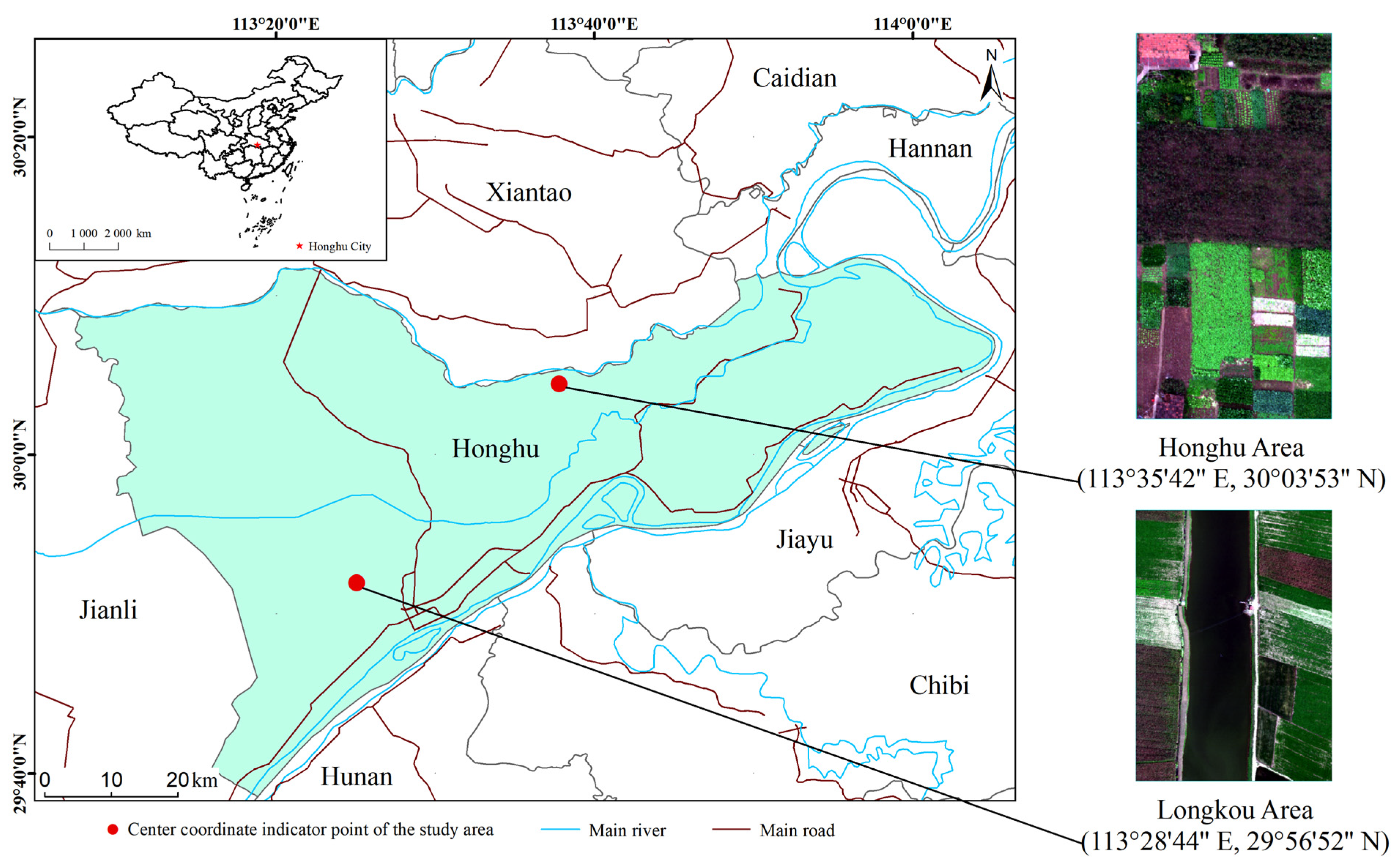
The two regions selected for this study are both located in Honghu City, Jingzhou City, Hubei Province, China. Honghu City is located at the southeastern end of the Jianghan Plain, spanning from 113°07′ to 114°05′ east of the Greenwich Meridian and 29°39′ to 30°12′ north of the Equator. It has a subtropical humid monsoon climate. The crop planting scale is small, and land fragmentation is common, in the two study areas [22]. The location of the study area is shown in Figure 1.
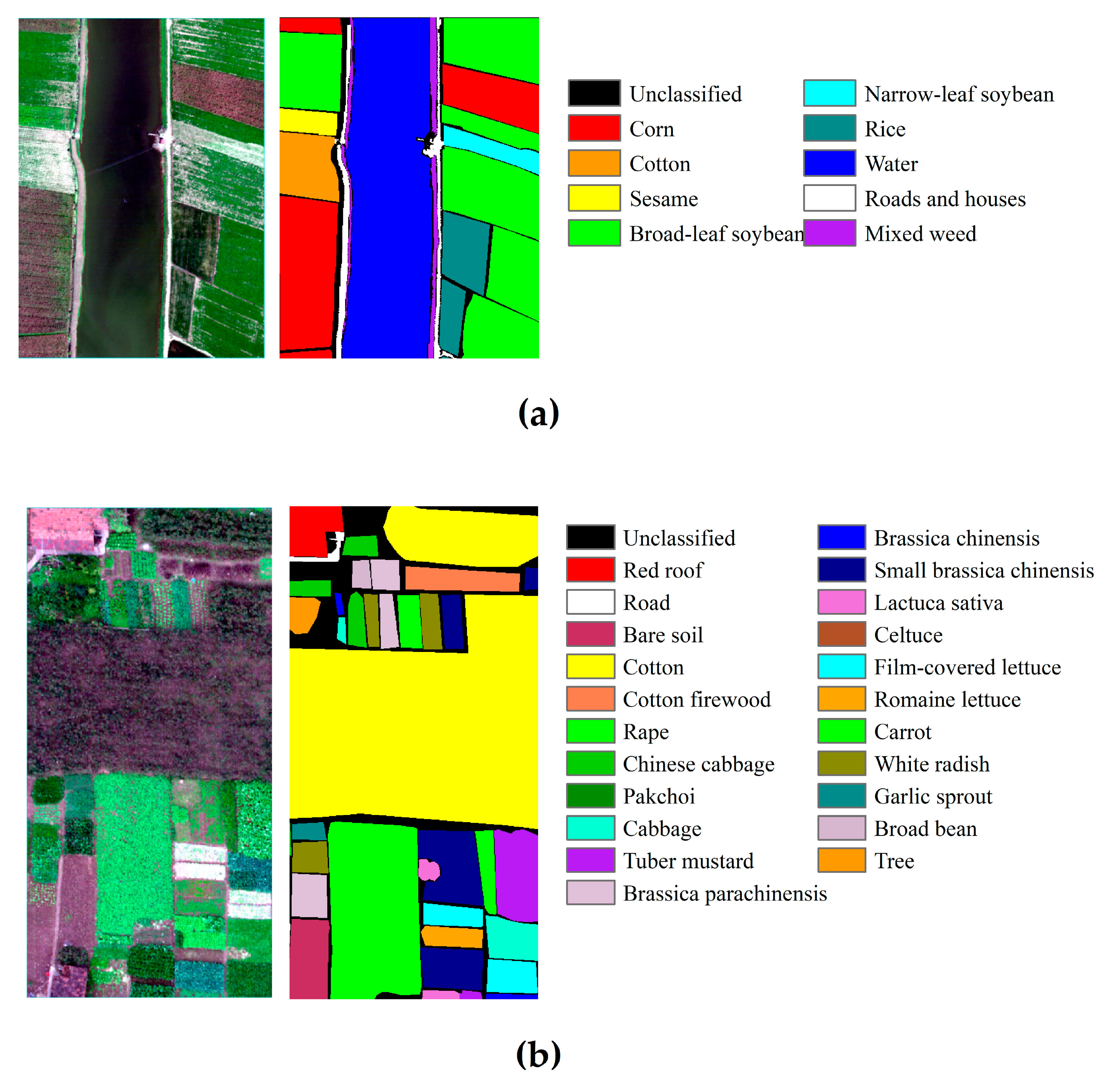
The original dataset used in this study is the UAV-borne Hyperspectral Image (WHU-HI) dataset, which contains two separate UAV-borne hyperspectral datasets: WHU-HI-Long Kou and WHU-HI-HongHu [23,24]. All datasets were obtained in the agricultural areas of different crop types in Honghu City through the Headwall Nano-Hyperspec sensor installed on the UAV platform, and all preprocessing processes, such as radiometric calibration and geometric correction, were completed in the HyperSpec software. The image sizes of the two datasets were 254.650 m × 185.200 m and 40.420 m × 20.425 m, respectively; there were 270 bands between 400 and 1000 nm. The spatial resolutions of the two sets of UAV hyperspectral images were 0.463 m and 0.043 m, respectively. The Longkou and Honghu areas each contained 9 types of ground objects and 22 types of ground objects, among which crops accounted for 6 types and 18 types, respectively. To avoid the interference of other ground objects in crop classification, the classification of other ground objects was carried out at the same time. A real land type survey of the study area is shown in Figure 2.
3. Research Methods
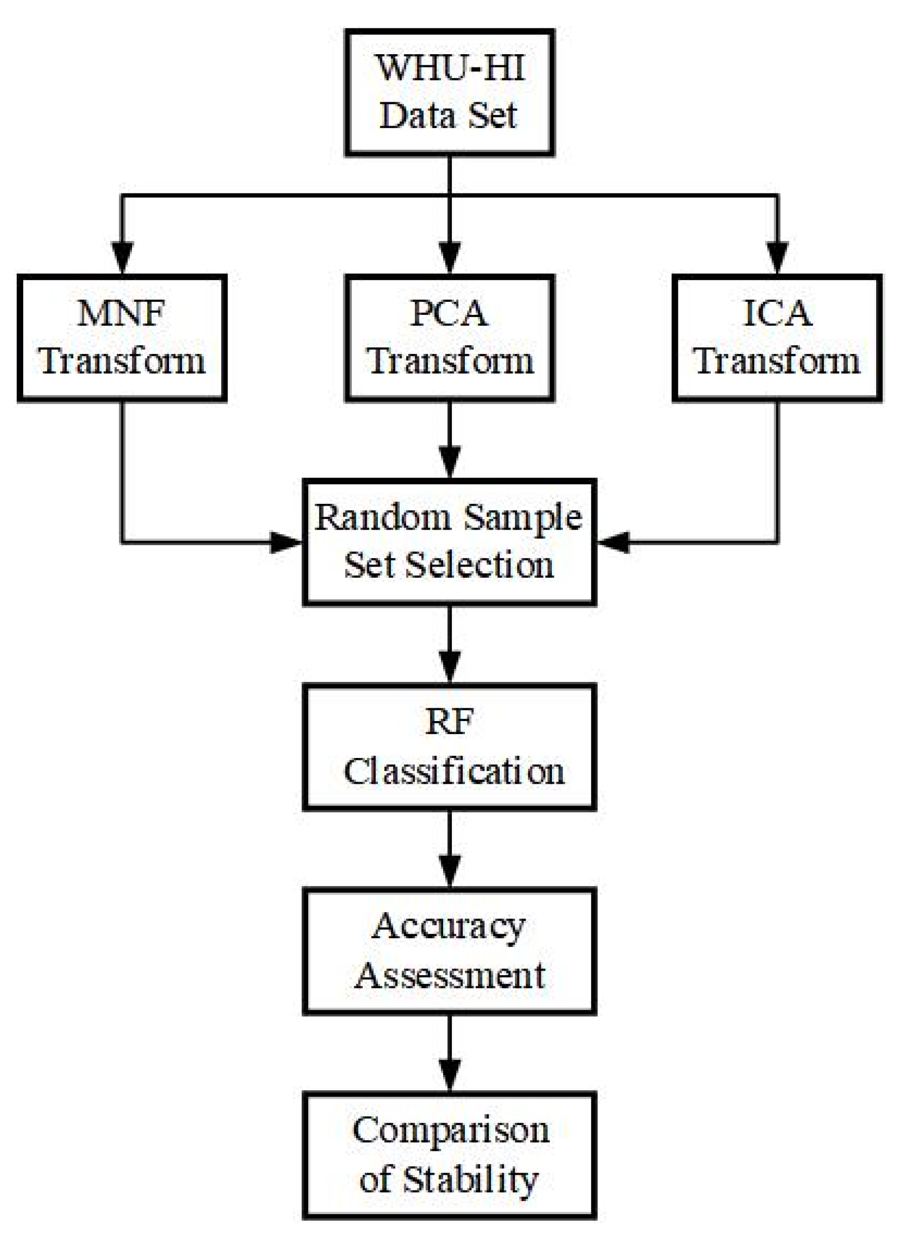
The main research route of this study is as Figure 3: MNF, PCA, and ICA feature transforms were carried out using WHU-HI data sets, and then random sample sets were selected using the results of the three feature transforms. Seven random sample sets of Train25–Train300 were selected, and then random forest classification was carried out. Finally, accuracy evaluation and stability comparison were carried out on the classification results.
3.1. Sample Acquisition Strategy and Accuracy Assessment Method
Samples can provide numerical feature information about categories for the supervised classification process, and the number and distribution of random sample points can have a great impact on the classification results. Therefore, sample selection is a key step in the subsequent classification process. The sample acquisition strategy of this study was to select a certain number of random points—that is, randomly select different numbers of random sample points, increasing from 25 to 300 for each type of ground object (25, 50, 100, 150, 200, 250, 300)—to generate seven random sample sets (referred to as Train25–Train300). In this study, a confusion matrix was used to evaluate the accuracy of the classification results, and the accuracy of each classification result was presented in the confusion matrix to compare the classification results with the true ground information.
3.2. Feature Transform
In this study, feature transform was performed first, and most of the feature information of the original image was concentrated into a few bands, thereby significantly reducing the processing time of the subsequent classification process [25]. This study compared the effects of different feature transforms, including the PCA transform, MNF transform, and ICA transform. The basic principle of the PCA transform is to concentrate the main information in the image data into a few bands to filter out redundant information so that the subsequent classification processing can be carried out smoothly [26]. MNF transform is a linear transform created by superimposing two PCA transforms [27]. The MNF transform adjusts and distinguishes noise through the covariance matrix in the PCA transform and then transforms the noise-whitening data. Considering the influence of noise, a better transform effect can be achieved when there is noise in the data [28,29,30]. The ICA transform can convert hyperspectral data into independent components to better complete the discovery and separation of hidden noise in the image, dimensionality reduction, noise reduction, anomaly detection, classification and spectral endmember extraction, and data fusion [31].
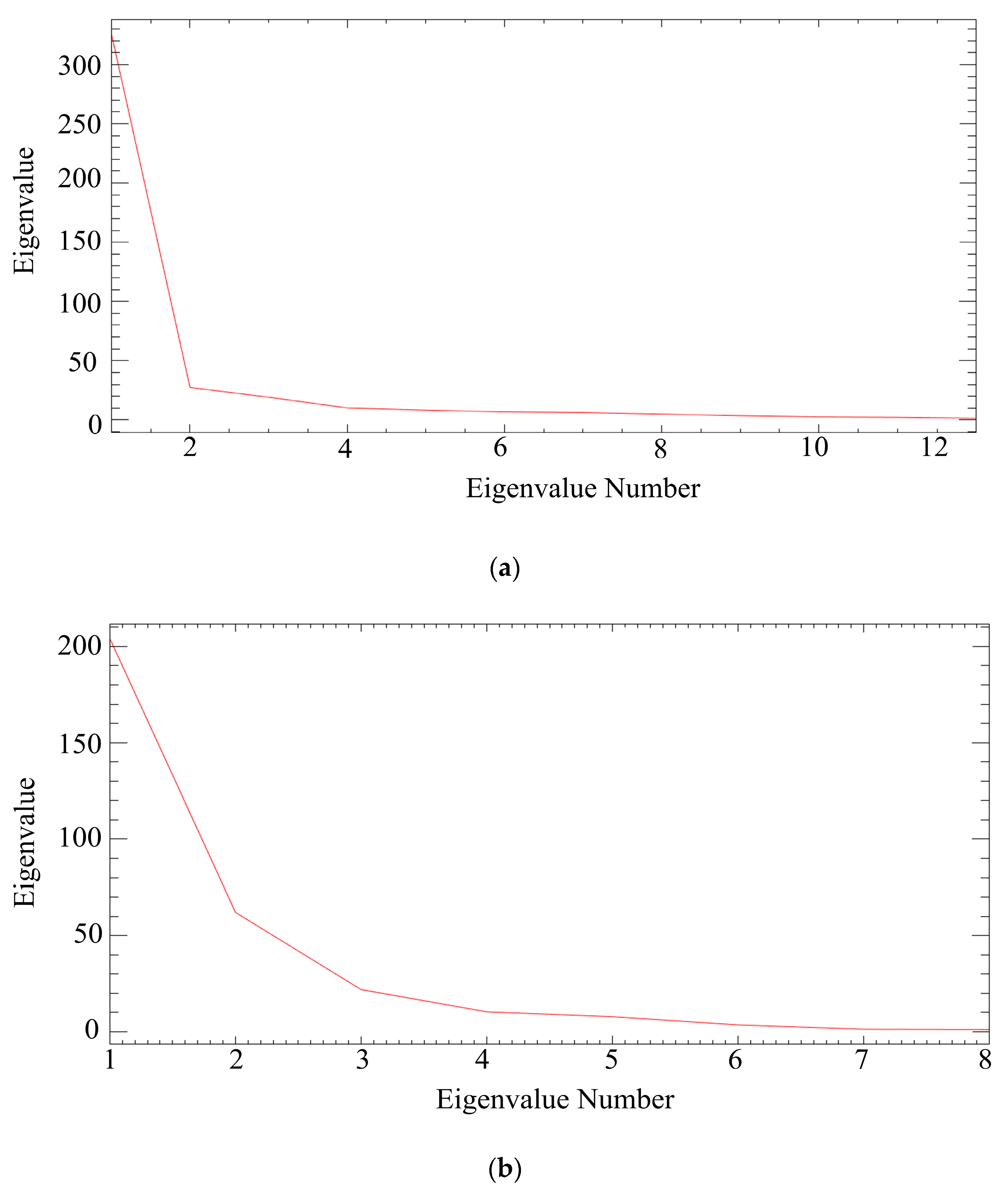
In the eigenvalue curve corresponding to the transformed image, as the number of eigenvalues increases, each eigenvalue gradually decreases until it converges to a certain constant. At this time, the transformed image reaches the best state, that which contains as much information as possible under the number of eigenvalues. Because of this, the band images after the eigenvalues corresponding to the convergent constants can be screened out to avoid too much redundant band information affecting the subsequent classification process.
MNF, PCA, and ICA transforms were carried out on the original data. Combined with the display status of band information after feature transform, the effective feature information was further screened, and the best ideal transform image was explored. To ensure the accuracy of the ideal band selection work, first, the derivative analysis method was used to screen the curve. When the derivative of the curve was 0, its eigenvalues converged to a stable value, and the corresponding number of bands at this time was the preliminarily determined ideal band. The number was set to N here. Second, verification work was carried out, and the image information at the (N + 1) band was presented separately for verification. If the corresponding information amount was small, it was finally determined that the N band was ideal for the transformed band.
3.3. Principle of the RF Classifier
The RF classifier, first proposed by Breiman, is a combined classifier obtained by taking the decision tree as the basic unit and performing ensemble learning through multiple combinations [32]. In the application of remote sensing image classification and change detection, it has obtained better experimental results than other classification algorithms because of its advantages of high accuracy, few parameters, and strong robustness [33].
The basic principle is to extract K sample subsets from the training sample set by the Bootstrap method. The value of K usually takes the number of sample subsets corresponding to when the out-of-bag error begins to converge to obtain the model with the best classification accuracy and generalization ability. The number of random features for node splitting m is usually taken as (M is the dimension of the feature vector). According to the value of m, a decision tree model is established for the K sample subsets. By classifying all the samples to be classified, the classification result sequence is obtained. The final classification result is determined by majority voting [32,34]. The basic formula of the final classification decision process is as follows:
In the formula, H(x) represents the final classification decision of the random forest, hi(x) represents the classification result of a single decision tree model, Y represents the output variable (target variable), and I(.) represents the indicative function.
The basic steps of RF algorithm classification in this study were as follows:
- (1)
- First, m feature variables were selected from all features using the square root method.
- (2)
- Second, m characteristic variables were used to establish a decision tree for the random sample (Train25–Train300).
- (3)
- The above two steps were repeated K times, that is, K decision trees were generated to form a random forest.
- (4)
- Finally, using the decision results of each decision tree, the category of final prediction was determined through the voting method.
In the actual classification process using an RF classifier, the number of trees N and the number of randomly selected feature variables M are the main factors determining the classification accuracy [35,36]. Through multiple parameter debugging and comparative analysis of classification experiments, the number of decision trees was determined to be 100, and the number of randomly selected feature variables was the square root of the number of bands of each image to be classified.
4. Results and Analysis
4.1. Feature Transform
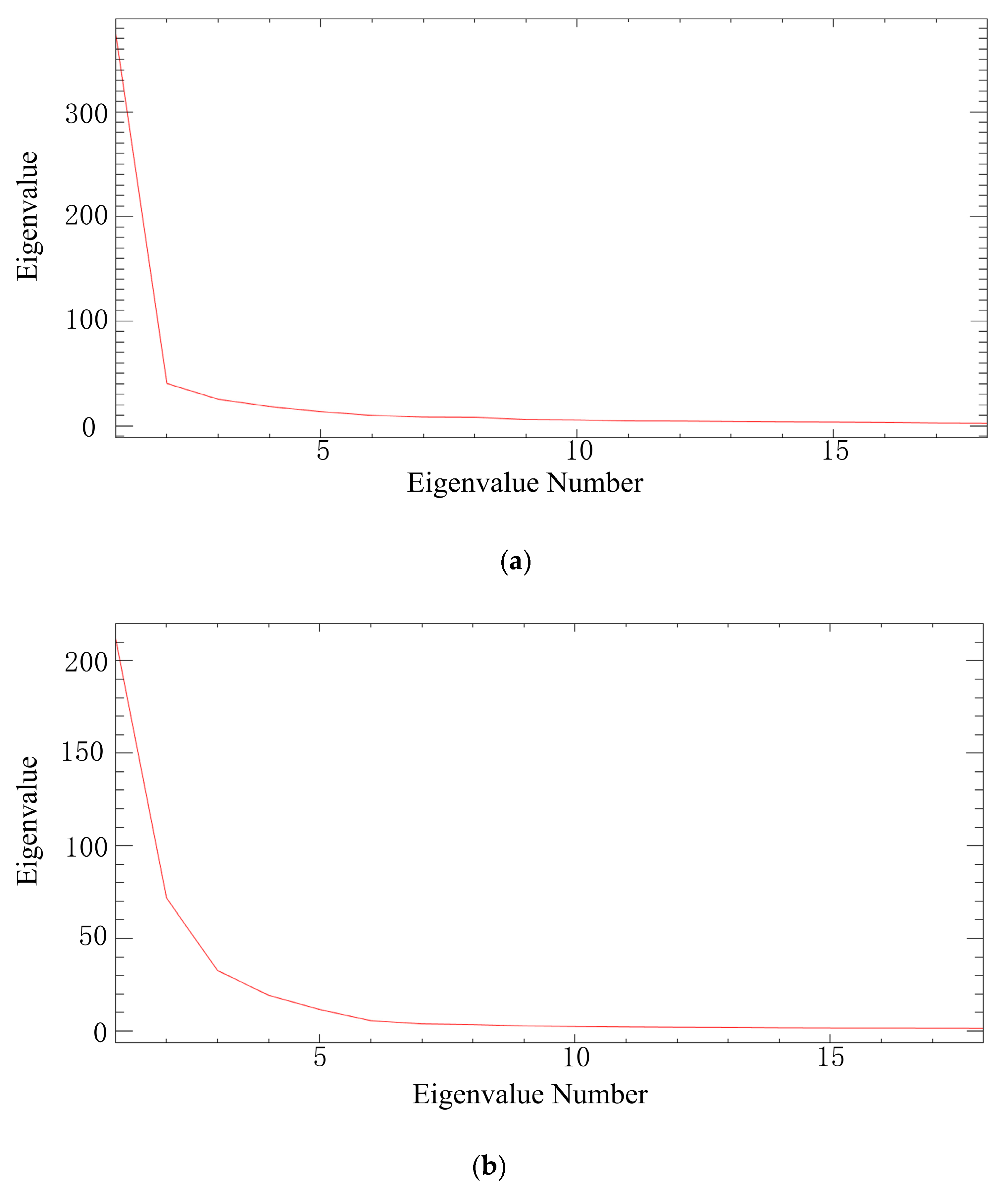
Figure 4 shows the characteristic curve of the MNF transform. The derivative values of the curves in the Longkou and Honghu areas were 0 when the number of eigenvalues is 18. The corresponding eigenvalues were 2.45 and 1.52, respectively, and the eigenvalue changes tended to be stable.
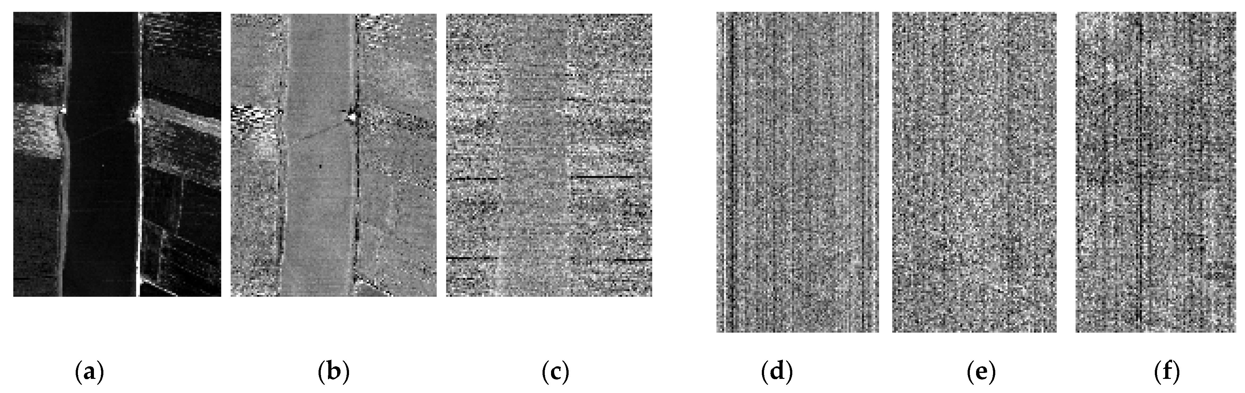
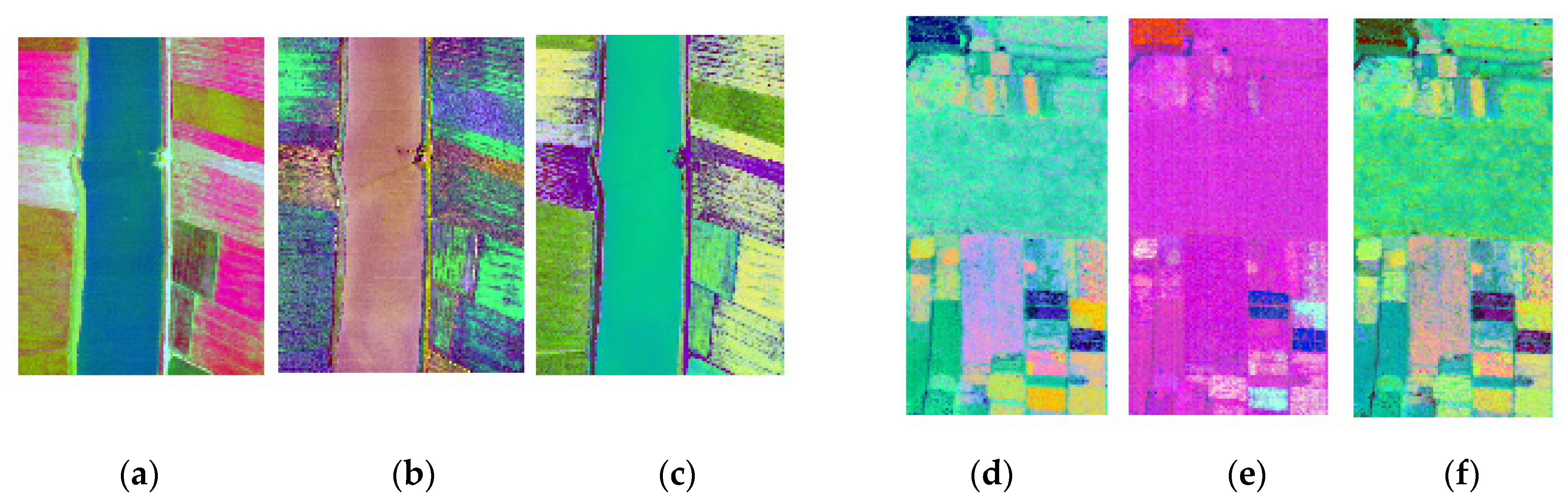
As shown in the curves in Figure 5, the PCA transform eigenvalue curves of the two regions converged at the 12th and 8th bands, respectively. Figure 6 shows the display status of the image information corresponding to each transformed (N + 1) band. There was little information after the 18 bands of MNF transformation in these two regions, so the optimal ideal bands for the MNF transform in the two regions were both 18 bands. Similarly, the optimal ideal bands for the PCA transform in Longkou and Honghu regions were 12 bands and 8 bands, respectively, and the optimal ideal bands for the ICA transform were 18 bands and 44 bands, respectively. Figure 7 is a color image composed of the first three components of each transform.
4.2. Accuracy Assessment
The final accuracy evaluation is shown in Table 1 and Table 2, which show that the classification accuracy of the two regions was affected by many factors.
In this study, the number of categories and the clarity of category boundaries had impacts on classification accuracy. The Longkou area had fewer categories and clearer boundaries between categories, and the highest classification accuracy of the random sample set was 97.18%, which was 6.12% higher than the best overall accuracy of 91.06% for the same RF classification algorithm with only four plantings [18]. On the other hand, the Honghu area had many categories and complex feature information, and the highest classification accuracy of the random sample set was 80.43%.
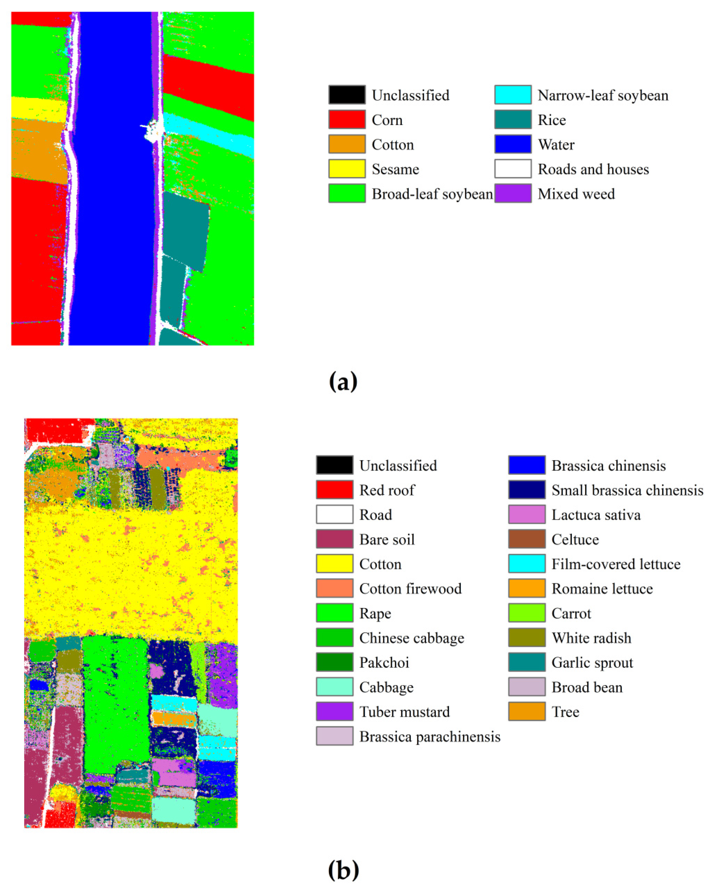
The characteristic of the MNF transform is that two PCA transforms are carried out considering the influence of noise, which has significant advantages when the category situation is more complex. The classification accuracy of different random sample sets in the two regions showed that the MNF–RF combination had higher classification accuracy than the other classification combinations. For random sample sets with the same numbers of sample points, the MNF–RF classification accuracy (95.66%) in the Longkou area was higher than that of the original image (80.14%), with a maximum improvement of 15.52%, and the MNF–RF classification accuracy (71.91%) in the Honghu area was higher than that of other classification combinations (54.48%), with a maximum improvement of 17.42%.
The image classification effect of PCA transform and ICA transform is greatly affected by the category information of the study area. For the Longkou area, where the category information was relatively simple, the RF classification accuracy of the image after feature transform was higher than that of the original image. Comparing the classification accuracy of different random sample sets in Table 1, the classification accuracy of the PCA transform was more ideal than that of the ICA transform. The classification information in the Honghu area was relatively complex. In Table 2, the classification accuracy of the image after MNF transform was higher than that of the original image, but the accuracy of the images after PCA and ICA transforms was lower than that of the original image. Furthermore, because the sample points of the random sample set were selected randomly, the advantages of the ICA and PCA transforms were not obvious. To sum up, the best classification combination for the random sample sets in the two regions was determined as the MNF–RF combination, and the best classification effect of the two regions is shown in Figure 8.
4.3. Comparison of Stability
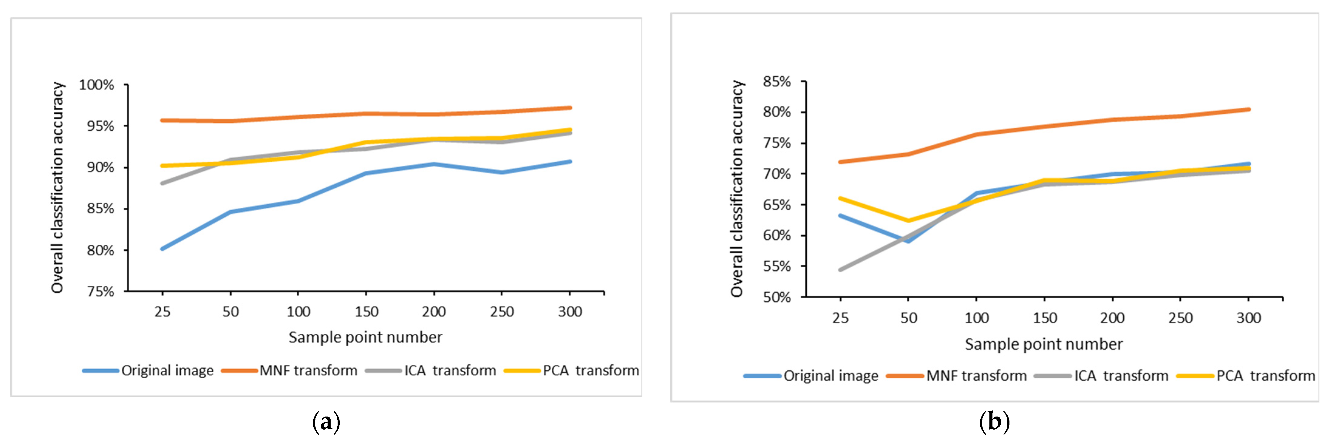
As shown in Figure 9, the curves of the two regions reflected the following characteristics. The overall classification accuracy was positively correlated with the fluctuation of the number of random sample points. The overall classification accuracy of RF classification after feature transformation showed a gentler trend with the number of sample points than the original image and was less affected by the number of sample points. MNF–RF curves in both figures were the smoothest, indicating that MNF–RF was least affected by the number of random sample points, followed by PCA–RF and ICA–RF. The overall classification accuracy fluctuations of MNF–RF in the two regions were less than 0.50% and 3.25%, respectively.
5. Conclusions
Accurate crop classification mapping is an important basis for agricultural production management, agricultural policymaking, and food safety and can provide necessary reference information for agricultural decision-making. Realizing efficient and accurate crop classification is a key step for structural optimization and management plan formulation. It is hoped that the research methods and ideas of this study can provide a reference for the development and structural adjustment of precision agriculture in other countries.
In this study, the MNF–RF combination, which was superior to the ICA–RF and PCA–RF combinations, was the best classification combination in practical application. The best classification accuracies of the MNF–RF random sample set in the two regions were 97.18% and 80.43%, respectively, which were 6.43% and 8.81% higher than the RF classification accuracy of the original image.
The MNF transform takes into account the influence of noise in UAV hyperspectral images to a large extent and has high stability in the face of a different number of random sample points. Therefore, while the curve of RF overall classification accuracy changed with the number of random sample points in the two regions, the MNF transform curve was the gentlest. The overall classification accuracies of MNF–RF in the Longkou and Honghu areas varied by less than 0.50% and 3.25%, respectively, with the fluctuation of sample points.
In conclusion, it is feasible to use the MNF–RF classification combination to perform fine crop classification using UAV hyperspectral image data. In actual use, the MNF–RF combination classification can be used to select fewer random sample points to complete the fine classification of crops with high precision, accuracy, and stability. This reduces the sampling workload, greatly improves efficiency, and saves much manpower and material resources.
In future research work, the impact of different classification combinations and random sample numbers on the individual classification accuracy of each crop can be clarified. In follow-up work, we can further compare the performance of RF classification with that of neural networks and support vector machines using the same transformations as employed with the RF classifier.
Author Contributions
Conceptualization: Zhihua Wang, Zhan Zhao; Methodology: Zhihua Wang, Zhan Zhao; Formal analysis and investigation: Zhihua Wang, Zhan Zhao, Chenglong Yin; Writing—original draft preparation: Zhihua Wang; Writing—review and editing: Zhihua Wang, Zhan Zhao, Chenglong Yin; Resources: Zhan Zhao; Supervision: Zhan Zhao. All authors have read and agreed to the published version of the manuscript.
Funding
This work was funded by the National Science and Technology Fundamental Resources Survey Project (2019FY202502).
Institutional Review Board Statement
Not applicable.
Informed Consent Statement
Not applicable.
Data Availability Statement
Not applicable.
Acknowledgments
Thanks to the RSIDEA team of the State Key Laboratory of Surveying, Mapping, and Remote Sensing Information Engineering, Wuhan University, which constructed a set of publicly shared hyperspectral and high-spatial resolution remote sensing imagery and ground object fine classification data set: WHU-HI. We thank Professor Kunshan Chen of Guilin University of Technology and Associate Professor Ying Yang of Nanjing University of Science and Technology for the cultivation of the first author’s logical thinking which has promoted the further perfection of the paper. We would like to express our gratitude and respect to the editors and anonymous reviewers for their valuable comments and suggestions, which helped improve the manuscript greatly.
Conflicts of Interest
The authors declare no conflict of interest.
References
- Weiguang, G. Practice and Application of Information Technology in Precision Agriculture—Review of Low-Altitude Remote Sensing Technology and Its Application in Precision Agriculture. Chin. J. Agric. Resour. Reg. Plan. 2021, 42, 144–152. [Google Scholar]
- Cai, Y.; Guan, K.; Peng, J.; Wang, S.; Seifert, C.; Wardlow, B.; Li, Z. A high-performance and in-season classification system of field-level crop types using time-series Landsat data and a machine learning approach. Remote Sens. Environ. 2018, 210, 35–47. [Google Scholar] [CrossRef]
- Wei, L.; Yu, M.; Zhong, Y.; Zhao, J.; Liang, Y.; Hu, X. Spatial–Spectral Fusion Based on Conditional Random Fields for the Fine Classification of Crops in UAV-Borne Hyperspectral Remote Sensing Imagery. Remote Sens. 2019, 11, 780. [Google Scholar] [CrossRef] [Green Version]
- Qingzhan, Z.; Ping, J.; Xuewen, W.; Lihong, Z.; Jianxin, Z. Classification of Protection Forest Tree Species Based on UAV Hyperspectral Data. Trans. Chin. Soc. Agric. Mach. 2021, 52, 190–199. [Google Scholar]
- Hui, L.; Jing, H.; Junjie, L. Monitoring of Corn Canopy Blight Disease Based on UAV Hyperspectral Method. Spectrosc. Spectr. Anal. 2020, 40, 1965–1972. [Google Scholar]
- Pascucci, S.; Pignatti, S.; Casa, R.; Darvishzadeh, R.; Huang, W. Special Issue “Hyperspectral Remote Sensing of Agriculture and Vegetation”. Remote Sens. 2020, 12, 3665. [Google Scholar] [CrossRef]
- Fei, S.; Yu, X.; Lan, M.; Li, L.; Xia, X.; He, Z.; Xiao, Y. Research on Winter Wheat Yield Estimation Based on Hyperspectral Remote Sensing and Ensemble Learning Method. Sci. Agric. Sin. 2021, 54, 3417–3427. [Google Scholar]
- Liu, Y.; Zhang, G.; Wang, X.; Zhou, C.; Yang, Z.; Wu, X.; Zhang, J. Classification study of Mikania micrantha kunth from UAV hyperspectral image band selection. Bull. Surv. Mapp. 2020, 4, 34–39. [Google Scholar] [CrossRef]
- Li, P.; Zhang, X.; Wang, W.; Zheng, H.; Yao, X.; Zhu, Y.; Cao, W.; Cheng, T. Assessment of Terrestrial Laser Scanning and Hyperspectral Remote Sensing for the Estimation of Rice Grain Yield. Sci. Agric. Sin. 2021, 54, 2965–2976. [Google Scholar]
- Lan, Y.; Zhu, Z.; Deng, X.; Lian, B.; Huang, J.; Huang, Z.; Hu, J. Monitoring and classification of citrus Huanglongbing based on UAV hyperspectral remote sensing. Trans. Chin. Soc. Agric. Eng. 2019, 35, 92–100. [Google Scholar]
- Okwuashi, O.; Ndehedehe, C.E. Deep support vector machine for hyperspectral image classification. Pattern Recognit. 2020, 103, 107298. [Google Scholar] [CrossRef]
- Wang, C.; Zhao, Q.; Ma, Y.; Ren, Y. Crop Identification of Drone Remote Sensing Based on Convolutional Neural Network. Trans. Chin. Soc. Agric. Mach. 2019, 50, 161–168. [Google Scholar]
- Du, P.; Xia, J.; Xue, Z.; Tan, K.; Su, H.; Bao, R. Review of hyperspectral remote sensing image classification. J. Remote Sens. 2016, 20, 236–256. [Google Scholar] [CrossRef]
- Fang, X.; Wen, Z.; Chen, J.; Wu, S.; Huang, Y.; Ma, M. Remote sensing estimation of suspended sediment concentration based on Random Forest Regression Model. Natl. Remote Sens. Bull. 2019, 23, 756–772. [Google Scholar]
- Yang, X.; Su, H.; Li, W.E.; Huang, L.; Wang, X.; Yan, X. Seasonal-spatial variations in satellite-derived global subsurface temperature anomalies. Natl. Remote Sens. Bull. 2019, 23, 997–1010. [Google Scholar]
- Wang, L.; Kong, Y.; Yang, X.; Xu, Y.; Liang, L.; Wang, S. Classification of land use in farming areas based on feature optimization random forest algorithm. Trans. Chin. Soc. Agric. Eng. 2020, 36, 244–250. [Google Scholar]
- Li, H.; Wang, L.; Xiao, S. Random forest classification of land use in hilly and mountaineous areas of southern China using multi-source remote sensing data. Trans. Chin. Soc. Agric. Eng. 2021, 37, 244–251. [Google Scholar]
- Yang, H.; Du, J.; Ruan, P.; Zhu, X.; Liu, H.; Wang, Y. Vegetation Classification of Desert Steppe Based on Unmanned Aerial Vehicle Remote Sensing and Random Forest. Trans. Chin. Soc. Agric. Mach. 2021, 52, 186–194. [Google Scholar]
- Hughes, G. On the mean accuracy of statistical pattern recognizers. IEEE Trans. Inf. Theory 1968, 14, 55–63. [Google Scholar] [CrossRef] [Green Version]
- Richter, R.; Reu, B.; Wirth, C.; Doktor, D.; Vohland, M. The use of airborne hyperspectral data for tree species classification in a species-rich Central European forest area. Int. J. Appl. Earth Obs. Geoinf. 2016, 52, 464–474. [Google Scholar] [CrossRef]
- Dabiri, Z.; Lang, S. Comparison of Independent Component Analysis, Principal Component Analysis, and Minimum Noise Fraction Transformation for Tree Species Classification Using APEX Hyperspectral Imagery. ISPRS Int. J. Geoinf. 2018, 7, 488. [Google Scholar] [CrossRef] [Green Version]
- Sijing, Y.; Changqing, S.; Feng, C.; Leina, Z.; Changxiu, C.; Chao, Z.; Jianyu, Y.; Dehai, Z. Cultivated land health-productivity comprehensive evaluation and its pilot evaluation in China. Trans. Chin. Soc. Agric. Eng. 2019, 35, 66–78. [Google Scholar]
- Zhong, Y.; Hu, X.; Luo, C.; Wang, X.; Zhao, J.; Zhang, L. WHU-Hi: UAV-borne hyperspectral with high spatial resolution (H2) benchmark datasets and classifier for precise crop identification based on deep convolutional neural network with CRF. Remote Sens. Environ. 2020, 250, 112012. [Google Scholar] [CrossRef]
- Zhong, Y.; Wang, X.; Xu, Y.; Wang, S.; Jia, T.; Hu, X.; Zhao, J.; Wei, L.; Zhang, L. Mini-UAV-Borne Hyperspectral Remote Sensing: From Observation and Processing to Applications. IEEE Geosci. Remote Sens. Mag. 2018, 6, 46–62. [Google Scholar] [CrossRef]
- Bajwa, S.; Kulkarni, S. Hyperspectral Data Mining. In Hyperspectral Remote Sensing of Vegetation; CRC Press: London, UK, 2011. [Google Scholar]
- Jolliffe, I. Principal Component Analysis. In International Encyclopedia of Statistical Science; Lovric, M., Ed.; Springer: Berlin/Heidelberg, Germany, 2011; pp. 1094–1096. [Google Scholar]
- Green, A.; Berman, M.; Switzer, P.; Craig, M. A transformation for ordering multispectral data in terms of image quality with implications for noise removal. IEEE Trans. Geosci. Remote Sens. 1988, 26, 65–74. [Google Scholar] [CrossRef] [Green Version]
- Harsanyi, J.C.; Chang, C.-I. Hyperspectral image classification and dimensionality reduction: An orthogonal subspace projection approach. IEEE Trans. Geosci. Remote Sens. 1994, 32, 779–785. [Google Scholar] [CrossRef] [Green Version]
- Underwood, E. Mapping nonnative plants using hyperspectral imagery. Remote Sens. Environ. 2003, 86, 150–161. [Google Scholar] [CrossRef]
- Nascimento, J.; Bioucas-Dias, J. Vertex component analysis: A fast algorithm to unmix hyperspectral data. IEEE Trans. Geosci. Remote Sens. 2005, 43, 898–910. [Google Scholar] [CrossRef] [Green Version]
- Hyvarinen, A. Fast and robust fixed-point algorithms for independent component analysis. IEEE Trans. Neural Netw. 1999, 10, 626–634. [Google Scholar] [CrossRef] [Green Version]
- Breiman, L. Random forests. Mach. Learn. 2001, 45, 5–32. [Google Scholar] [CrossRef] [Green Version]
- Rodriguez-Galiano, V.F.; Ghimire, B.; Rogan, J.; Chica-Olmo, M.; Rigol-Sanchez, J.P. An assessment of the effectiveness of a random forest classifier for land-cover classification. ISPRS J. Photogramm. Remote Sens. 2012, 67, 93–104. [Google Scholar] [CrossRef]
- Zhang, Z.; Zhang, X.; Xin, Q.; Yang, X. Combining the Pixel-based and Object-based Methods for Building Change Detection Using High-resolution Remote Sensing Images. Acta Geod. Cartogr. Sin. 2018, 47, 102–112. [Google Scholar]
- Liu, S.; Jiang, Q.; Yue, M.A.; Xiao, Y.; Yuanhua, L.I.; Cui, C. Object-oriented Wetland Classification Based on Hybrid Feature Selection Method Combining with Relief F, Multi-objective Genetic Algorithm and Random Forest. Trans. Chin. Soc. Agric. Mach. 2017, 48, 119–127. [Google Scholar]
- Yun, H.E.; Huang, C.; He, L.I.; Liu, Q.; Liu, G.; Zhou, Z.; Zhang, C. Land-cover classification of random forest based on Sentinel-2A image feature optimization. Resour. Sci. 2019, 41, 992–1001. [Google Scholar]
Figure 1.
Location of the study area.

Figure 2.
(a) Survey map of real land types in the Longkou area; (b) survey map of real land types in the Honghu area.
Figure 2.
(a) Survey map of real land types in the Longkou area; (b) survey map of real land types in the Honghu area.

Figure 3.
Flow chart of study.

Figure 4.
(a) The MNF transform eigenvalue curve of the Longkou area; (b) the MNF transform eigenvalue curve of the Honghu area.
Figure 4.
(a) The MNF transform eigenvalue curve of the Longkou area; (b) the MNF transform eigenvalue curve of the Honghu area.

Figure 5.
(a) The PCA transform eigenvalue curve of the Longkou area; (b) the PCA transform eigenvalue curve of the Honghu area.
Figure 5.
(a) The PCA transform eigenvalue curve of the Longkou area; (b) the PCA transform eigenvalue curve of the Honghu area.

Figure 6.
(a–c) The MNF transform at 19 bands, ICA transform at 19 bands, and PCA transform at 13 bands, respectively, in the Longkou area; (d–f) the MNF transform at 19 bands, ICA transform at 45 bands, and PCA transform at 9 bands, respectively, in the Honghu area.
Figure 6.
(a–c) The MNF transform at 19 bands, ICA transform at 19 bands, and PCA transform at 13 bands, respectively, in the Longkou area; (d–f) the MNF transform at 19 bands, ICA transform at 45 bands, and PCA transform at 9 bands, respectively, in the Honghu area.

Figure 7.
(a–c) Images of the Longkou area after MNF, ICA, and PCA transforms, respectively; (d–f) images of the Honghu area after MNF, ICA, and PCA transforms, respectively.
Figure 7.
(a–c) Images of the Longkou area after MNF, ICA, and PCA transforms, respectively; (d–f) images of the Honghu area after MNF, ICA, and PCA transforms, respectively.

Figure 8.
(a) Classification results of the random sample set in the Longkou area; (b) classification results of the random sample set in the Honghu area.
Figure 8.
(a) Classification results of the random sample set in the Longkou area; (b) classification results of the random sample set in the Honghu area.

Figure 9.
(a) The change of overall classification accuracy with the number of random sample points in the Longkou area; (b) the change of overall classification accuracy with the number of random sample points in the Honghu area.
Figure 9.
(a) The change of overall classification accuracy with the number of random sample points in the Longkou area; (b) the change of overall classification accuracy with the number of random sample points in the Honghu area.


Table 1.
RF classification accuracy evaluation of random sample sets in the Longkou area.
| Random Sample Set | Original Image | MNF Transform | ICA Transform | PCA Transform |
|---|---|---|---|---|
| Train 25 | 80.14% | 95.66% | 88.12% | 90.27% |
| Train 50 | 84.68% | 95.65% | 90.98% | 90.56% |
| Train 100 | 85.95% | 96.08% | 91.82% | 91.27% |
| Train 150 | 89.27% | 96.49% | 92.24% | 93.06% |
| Train 200 | 90.46% | 96.43% | 93.41% | 93.43% |
| Train 250 | 89.42% | 96.68% | 93.11% | 93.53% |
| Train 300 | 90.75% | 97.18% | 94.17% | 94.62% |
Table 2.
RF classification accuracy evaluation of random sample sets in the Honghu area.
| Random Sample Set | Original Image | MNF Transform | ICA Transform | PCA Transform |
|---|---|---|---|---|
| Train 25 | 63.31% | 71.91% | 54.48% | 66.08% |
| Train 50 | 59.06% | 73.20% | 59.93% | 62.38% |
| Train 100 | 66.88% | 76.45% | 65.72% | 65.67% |
| Train 150 | 68.58% | 77.70% | 68.27% | 69.06% |
| Train 200 | 69.92% | 78.83% | 68.77% | 68.86% |
| Train 250 | 70.32% | 79.34% | 69.79% | 70.48% |
| Train 300 | 71.62% | 80.43% | 70.54% | 70.98% |
Publisher’s Note: MDPI stays neutral with regard to jurisdictional claims in published maps and institutional affiliations. |
© 2022 by the authors. Licensee MDPI, Basel, Switzerland. This article is an open access article distributed under the terms and conditions of the Creative Commons Attribution (CC BY) license (https://creativecommons.org/licenses/by/4.0/).
Share and Cite
MDPI and ACS Style
Wang, Z.; Zhao, Z.; Yin, C. Fine Crop Classification Based on UAV Hyperspectral Images and Random Forest. ISPRS Int. J. Geo-Inf. 2022, 11, 252. https://0-doi-org.brum.beds.ac.uk/10.3390/ijgi11040252
AMA Style
Wang Z, Zhao Z, Yin C. Fine Crop Classification Based on UAV Hyperspectral Images and Random Forest. ISPRS International Journal of Geo-Information. 2022; 11(4):252. https://0-doi-org.brum.beds.ac.uk/10.3390/ijgi11040252
Chicago/Turabian StyleWang, Zhihua, Zhan Zhao, and Chenglong Yin. 2022. "Fine Crop Classification Based on UAV Hyperspectral Images and Random Forest" ISPRS International Journal of Geo-Information 11, no. 4: 252. https://0-doi-org.brum.beds.ac.uk/10.3390/ijgi11040252
Note that from the first issue of 2016, this journal uses article numbers instead of page numbers. See further details here.