Article

An Integrated Graph Model for Spatial–Temporal Urban Crime Prediction Based on Attention Mechanism

1
School of Information Technology and Cyber Security, People’s Public Security University of China, Beijing 100038, China
2
School of Emergency Management and Safety Engineering, China University of Mining and Technology, Beijing 100083, China
3
Safety and Security Science Section, Faculty of Technology, Policy and Management, TU Delft, 2628 BX Delft, The Netherlands
*
Author to whom correspondence should be addressed.
ISPRS Int. J. Geo-Inf. 2022, 11(5), 294; https://0-doi-org.brum.beds.ac.uk/10.3390/ijgi11050294
Submission received: 28 March 2022 / Revised: 19 April 2022 / Accepted: 26 April 2022 / Published: 30 April 2022

Abstract

:
Crime issues have been attracting widespread attention from citizens and managers of cities due to their unexpected and massive consequences. As an effective technique to prevent and control urban crimes, the data-driven spatial–temporal crime prediction can provide reasonable estimations associated with the crime hotspot. It thus contributes to the decision making of relevant departments under limited resources, as well as promotes civilized urban development. However, the deficient performance in the aspect of the daily spatial–temporal crime prediction at the urban-district-scale needs to be further resolved, which serves as a critical role in police resource allocation. In order to establish a practical and effective daily crime prediction framework at an urban police-district-scale, an “online” integrated graph model is proposed. A residual neural network (ResNet), graph convolutional network (GCN), and long short-term memory (LSTM) are integrated with an attention mechanism in the proposed model to extract and fuse the spatial–temporal features, topological graphs, and external features. Then, the “online” integrated graph model is validated by daily theft and assault data within 22 police districts in the city of Chicago, US from 1 January 2015 to 7 January 2020. Additionally, several widely used baseline models, including autoregressive integrated moving average (ARIMA), ridge regression, support vector regression (SVR), random forest, extreme gradient boosting (XGBoost), LSTM, convolutional neural network (CNN), and Conv-LSTM models, are compared with the proposed model from a quantitative point of view by using the same dataset. The results show that the predicted spatial–temporal patterns by the proposed model are close to the observations. Moreover, the integrated graph model performs more accurately since it has lower average values of the mean absolute error (MAE) and root mean square error (RMSE) than the other eight models. Therefore, the proposed model has great potential in supporting the decision making for the police in the fields of patrolling and investigation, as well as resource allocation.

1. Introduction

In recent years, spatial–temporal crime prediction technology has been rapidly developed. With deriving data that include the crime incidents number, population density, weather variables, etc., spatial–temporal patterns of assault, robbery, theft, or other types of crimes can be predicted with the help of machine learning (especially deep learning) and other methods [1,2,3,4,5,6,7,8]. It provides references and predictions about when and where the crime hotspot would be to the police in advance, so it contributes to crime prevention as well as better police resources allocations. With respect to practicality, the accuracy of crime prediction can be regarded as the most important indicator.
In order to establish accurate spatial–temporal crime prediction models, support vector machine (SVM), random forest (RF), and other machine learning algorithms were adopted to predict the spatial and temporal distributions of different types of crimes. For example, Ingilevich and Ivanov [9] made a comparative study about three predictive models (linear regression, logistic regression, and gradient boosting) and pointed out that the accuracy of the gradient boosting model (which is a typical machine learning model) was much higher than that of the other two statistics-based models. Yu et al. [10] proposed a new ST-cokriging method for crime prediction on weekly, biweekly, and quad-weekly scales, and the validation results showed that the minimum root mean square error (RMSE = 0.145) was on the weekly scale. Compared with spatial–temporal prediction, the time series prediction of crime has been studied by more scholars by using machine learning frameworks. Dash et al. [11] utilized various public city data to predict the time series of the crime incidents number of Chicago in the US, and reported that the prediction performance of the support vector regression was higher than that of the polynomial and auto-regressive methods. Chen et al. [12] applied a support vector machine method based on fuzzy information granulation to analyze and forecast the crime rates in a city of China, and the results indicated that the accuracy of this model is much better than that of ARIMA. Pillai [13] adopted machine learning models extreme gradient boosting (XGBoost), random forest, etc., to predict the violation and narcotics crimes in Chicago, and found that XGBoost outperformed all of the other models, with the highest R2 value of 88% and RMSE value of 2.57 towards crime incidents. In general, machine-learning-based methods are more successful in time series predictions than spatial–temporal predictions of crimes. One of the most important shortcomings may be that the ability of the spatial feature extraction of these models is inadequate.
In the last decades, deep neural networks became a fruitful approach to address the problems of complex feature engineering with their powerful self-learning capacity. Deep neural networks have been stimulated and widely applied in the fields of computer vision [14,15]. With deep learning, complicated spatial–temporal features of crimes can be captured and utilized to predict the future patterns of crimes. Li et al. [16] forecasted the yearly property crime incidents number of a city (with a spatial resolution of 100 m × 100 m) that is located in the south of China by using back propagation (BP) neural networks and genetic algorithms. Zhang et al. [17] studied the hourly prediction of crime patterns in the city of Suzhou in China based on the spatial–temporal residual networks (ST-ResNet) model: an adaptive spatial resolution method was proposed to find out the best spatial resolution for crime risk prediction, and the results pointed out that a 2.4 km spatial resolution can obtain the best performance for crime prediction (RMSE = 7.81). Qian et al. [18] established the GeST model based on grid division to predict the number of theft crimes in New York City from 2011 to 2018: the experimental result on the test set was better than ARIMA, LSTM, and other models. Zhang et al. [19] designed a new optimization modeling method for crime prediction based on the grid management concept by using a BP neural network algorithm, which was validated by the data of four different crimes in Chicago, and the results showed that the RMSE of this method fell by approximately 9% on average compared with the traditional meshless models. Han et al. [20] proposed an integrated model of crime prediction by combining LSTM with ST-GCN to forecast the spatial–temporal crime risk of urban communities in Chicago, and the result showed that this model had been verified by practical examples and achieved a superior prediction to Ridge, random forest, and LSTM models.
As reported by the previous literatures, deep learning methods seem to be more suitable for spatial–temporal crime prediction than the traditional machine learning algorithms. However, for the purposes of supporting decision making for the police, there are still three main gaps. Firstly, most of the previous studies focused on yearly, monthly, or weekly scales rather than a daily scale due to the insufficient accuracy of the models. A few studies focused on a daily (even hourly) scale, but usually obtained relatively larger errors in terms of RMSE or MAPE [9,10,16,17,18,19,20]. With respect to security inspection and patrolling, as well as other associated jobs, police may be more interested in the effective daily crime prediction results. Secondly, a considerable number of studies are based on regular spatial–temporal grids for spatial division [9,16,17,18,19], but this is inconsistent with actual administrative areas. Generally, policing strategies should be consistent within the same administrative area (such as the community or police district). As a risk compensation element, it may affect the spatial–temporal distribution of crimes. Thus, the grid-based deep learning frameworks may have limited accuracy in terms of spatial–temporal crime predictions. Thirdly, spatial–temporal crime prediction models should also pay attention to convenience and feasibility. However, most of the module connections of the present models are “offline”, which means that the spatial prediction module and the temporal prediction module are separated, not “online”. This may affect its convenience in practical applications.
To address these shortcomings, an “online” integrated graph model based on the attention mechanism for spatial–temporal crime prediction is proposed in this study. This model combines a residual neural network (ResNet), graph convolutional network (GCN), and LSTM to extract spatial–temporal features from the crime data. Moreover, the topological relationship among different urban districts is also captured, and the attention mechanism is incorporated into this model. The attention probability distribution can give high weight to the critical information while ruling out irrelevant information in the proposed model. Finally, feature fusion is completed through the weighted calculation of multiple features; meanwhile, the “offline” problem is solved as well. To validate this “online” integrated graph model, the daily theft and assault data in a police-district scale of the city of Chicago in the US from 1 January 2015, to 7 January 2020 are used. Indices of mean absolute error (MAE) and RMSE are employed to quantitatively evaluate this model. Furthermore, comparative analysis is also carried out in this study with other eight models applied in previous studies.
The rest of this paper is organized as follows. Section 2 describes the investigated area; presents the data used for the model validation; elaborates on the spatial–temporal crime prediction algorithm and the validation schemes. Section 3 is about the prediction results and discussions. Finally, Section 4 summarizes our main contributions and puts forward a set of recommendations for further study.

2. Materials and Methods

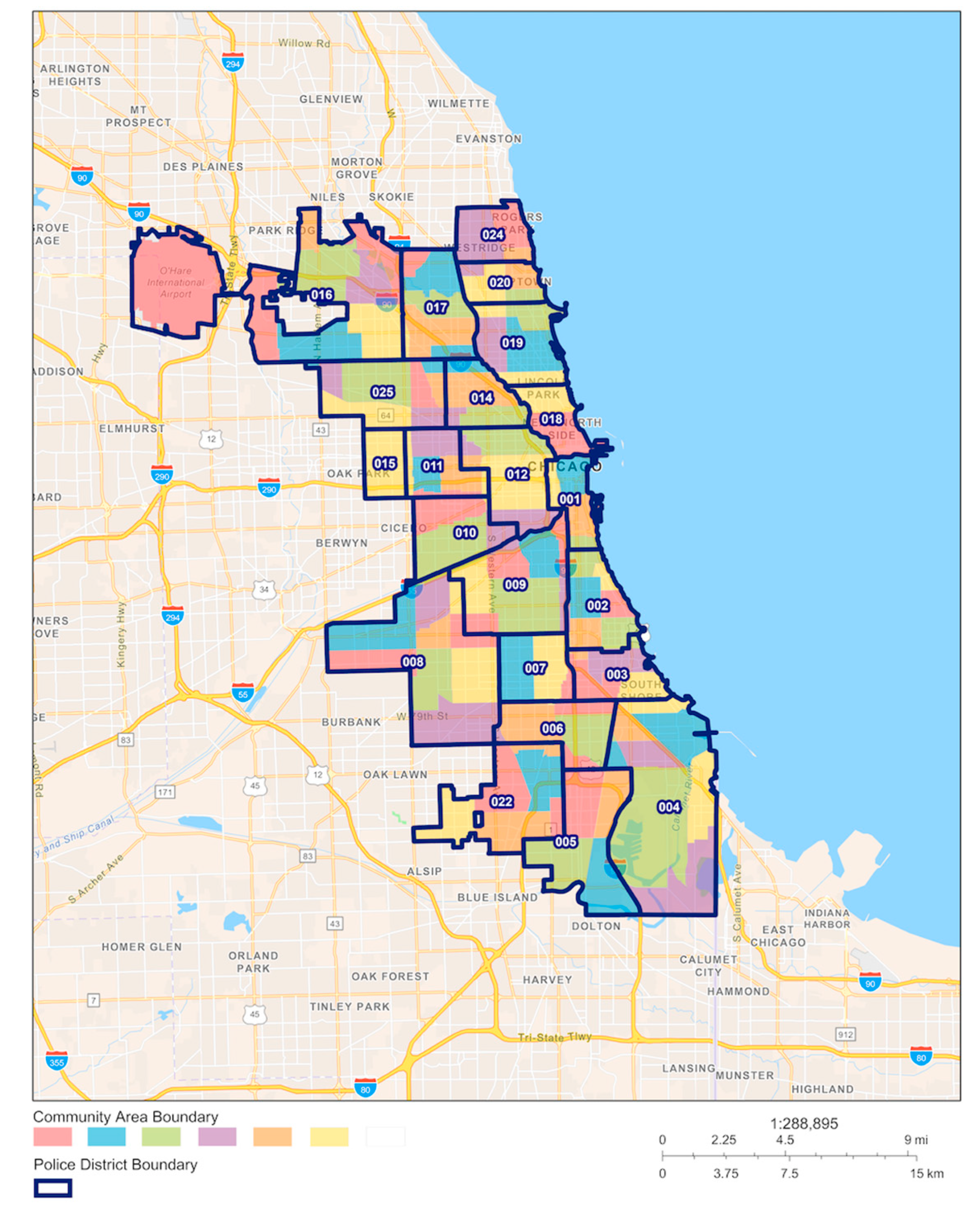
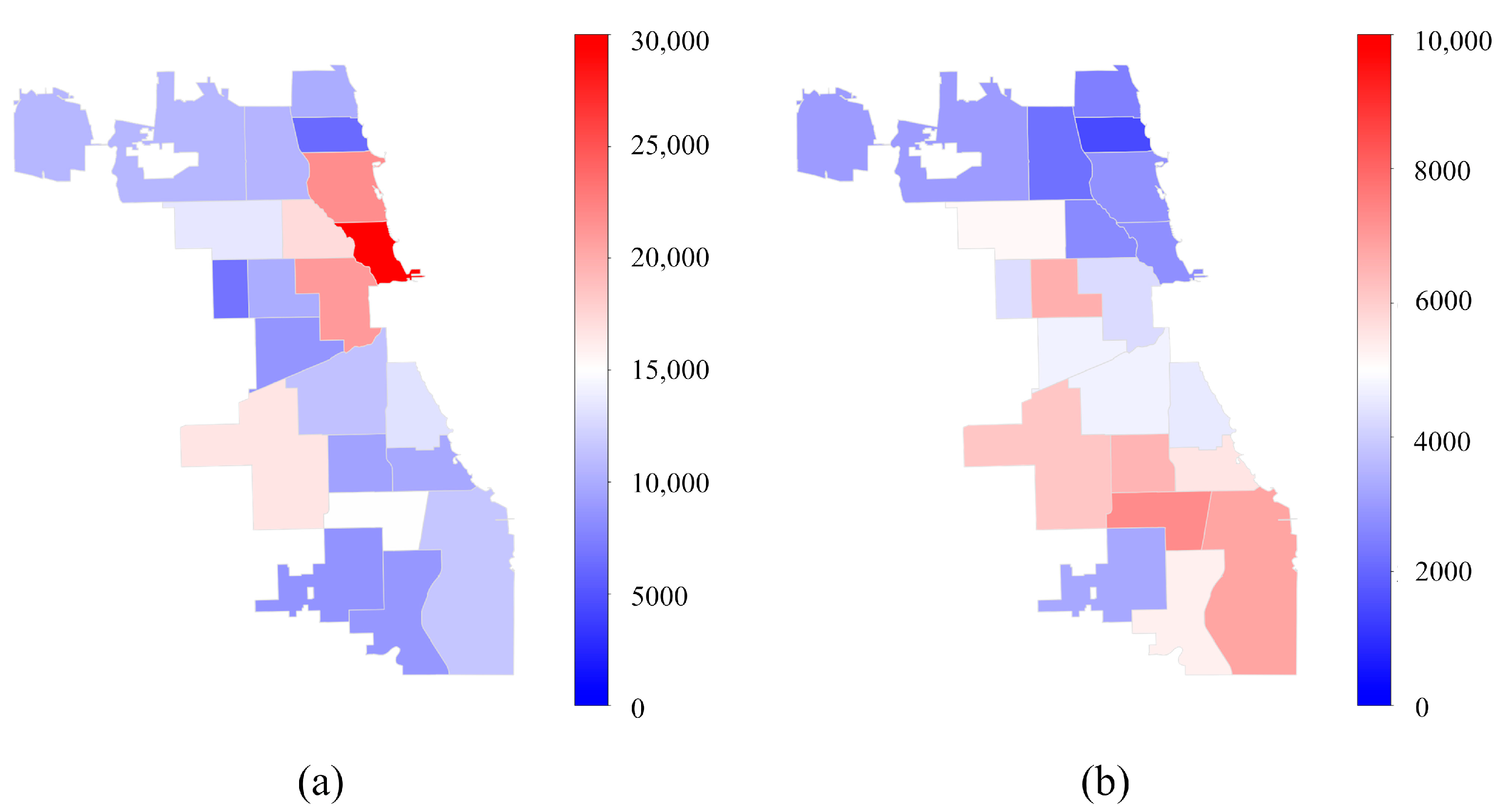
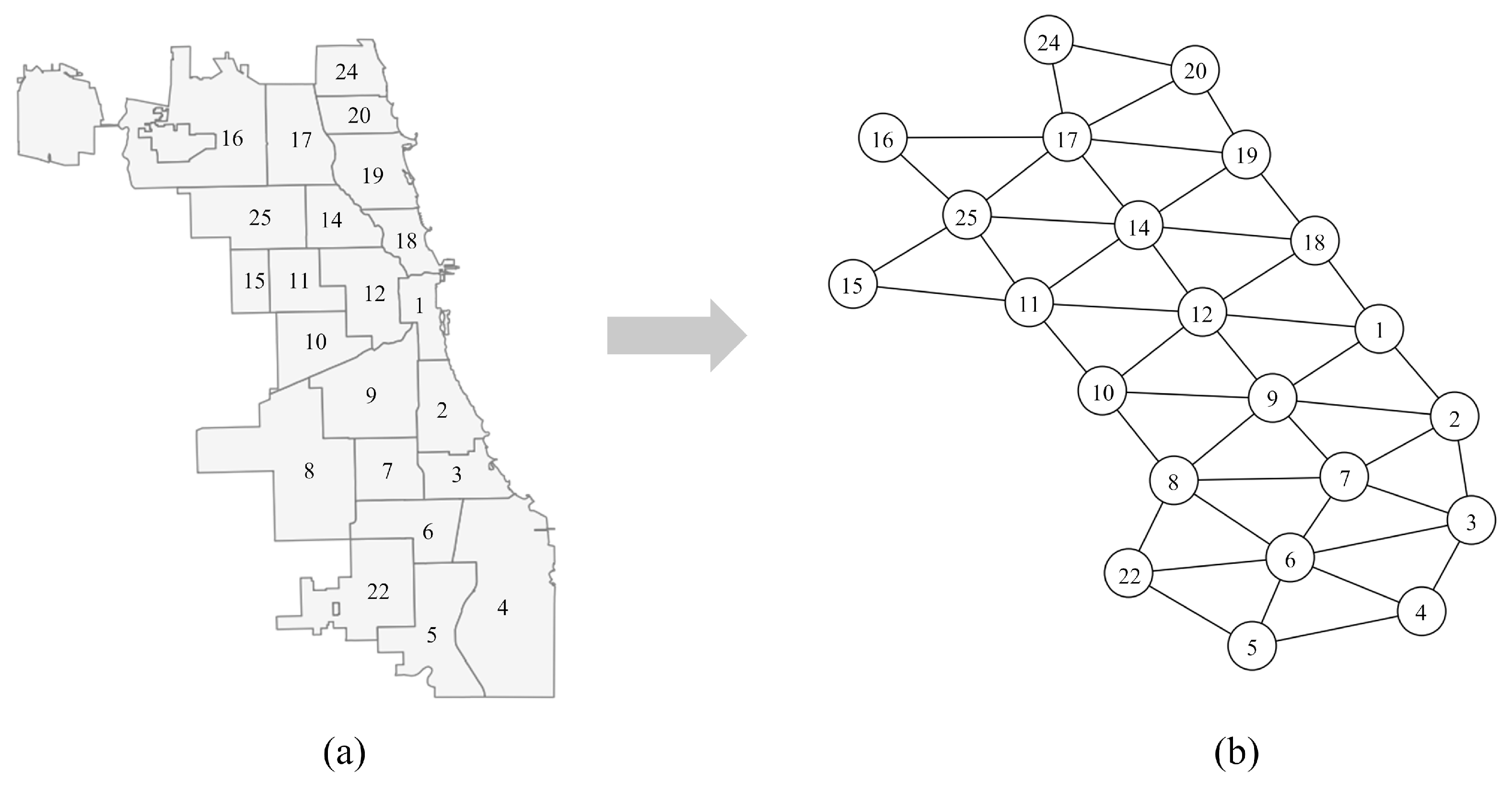
2.1. Study Area and Data Description

The city of Chicago was selected as the investigated area. It is the most densely populated city in Illinois, and the third-largest city in the United States, following New York City and Los Angeles. By the end of 2020, the estimated population of Chicago is 2,746,388 (Source: https://www.census.gov/, accessed on 1 October 2020). Chicago is in the center of the North American continent, and it is one of the most important international financial centers. As a typical large city, Chicago suffers from a large number of crimes, including the types of assaults, burglary, theft, etc., so it is very suitable for validating crime prediction models. A number of previous studies also chose this city to validate their proposed crime prediction methods, which can provide comparisons for this research.
This city has 22 police districts that overlap with 77 communities (as shown in Figure 1). In some of the police districts, one police station may serve multiple communities, while it is also possible that one community is covered by more than one police district. As the smallest cell of a city, the community is usually selected as the spatial unit to predict the spatial–temporal patterns of crime in previous studies [6,20,21,22,23]. However, in this study, spatial areas were divided by police districts. As is well known, crime risk is not only affected by population density, traffic environment, economic level, etc., but is also considerably influenced by the work of the police (such as patrolling, security check, etc.), which should be considered as a non-ignorable risk compensation factor. Within the same police district, the police strategy usually has spatial homogeneity. By contrast, the strategies may be varied between different police districts so that the impacts of police on crime risks may be quite different. This is why we chose police districts (rather than communities) to spatially divide the city. Another reason is that the spatial–temporal crime prediction results in a specific police district that can be applied directly to supporting the decision making with respect to police resource allocation within this district. As shown in Figure 1, the 22 police districts of Chicago are numbered from 1 to 25, excluding 13, 21, and 23, in which, the largest and the smallest police districts have areas of 816.6 km2 and 79.9 km2, respectively.
The dataset used for training and testing the established model was derived from the Chicago open data portal (https://data.cityofchicago.org/, accessed on 1 October 2020), which is a publicly available data search and exploration platform developed (and currently managed) by the University of Chicago’s Urban Center for Computation and Data. The crime data were collected from the “Crimes-2001 to present” dataset, a real-life collection of instances describing crime events in Chicago from 2001 to the present in which the repository is updated every week. From the “Crimes-2001 to present” dataset, we collected theft (as one of the typical property crimes) and assault (as one of the typical violent crimes) incidents numbers within the 22 police districts over five years (1833 days) from 1 January 2015, to 7 January 2020. In the data pre-processing stage, missing data were dropped, and the number of theft and assault incidents in the 22 police districts of Chicago was counted at a daily scale. A total of 404,269 pieces of valid data were finally obtained, including 308,020 pieces of theft data and 96,249 pieces of assault data. Figure 2 shows the temporal distribution of theft and assault incidents numbers in the 22 police districts of Chicago. As shown in Figure 2, both seasonality and daily variations of theft and assault can be observed.
Figure 3 shows the spatial patterns of theft and assault incidents numbers in Chicago. The theft incidents in Chicago are mainly concentrated in the northeast areas, whereas assault incidents are indicated by hot areas in the southeast. According to this figure, the accumulated theft number in the 18th police district reaches approximately 30000, which is much larger than that in other districts, indicating that theft has a significant spatial aggregation. The descriptive statistics of theft and assault incidents numbers in the 22 police districts are listed in Table A1. The number of theft incidents (M = 18.754, SD = 7.397) is larger than that of assault incidents (M = 1.939, SD = 1.472). Here, M is the crime incidents number’s mean value, and SD indicates the crime incidents number’s standard deviation.
Topological graph of the 22 police districts in Chicago was also used to train the model. According to the neighborhood relationship among police districts of Chicago, the topological map of adjacent police districts is obtained as shown in Figure 4.
Previous studies demonstrated that, besides the spatial–temporal features of crimes, weather variables are also used as external features to build the deep learning crime prediction models [20,22,24,25,26]. The reason is that the temperature and relative humidity proved to have relationships with some types of crimes, including assault, burglary, robbery, rape, and so on [27,28,29]. Heat stress indices can well capture the combination of the impacts of temperature and relative humidity on crime rates. Therefore, we chose the heat stress discomfort index (DI) [20,27,28] as one of the external features, and the description of DI is presented in Appendix B. Apart from DI, the features “Weekend” and “Holiday” were also applied as the external features. The descriptions of these features are listed in Table 1.

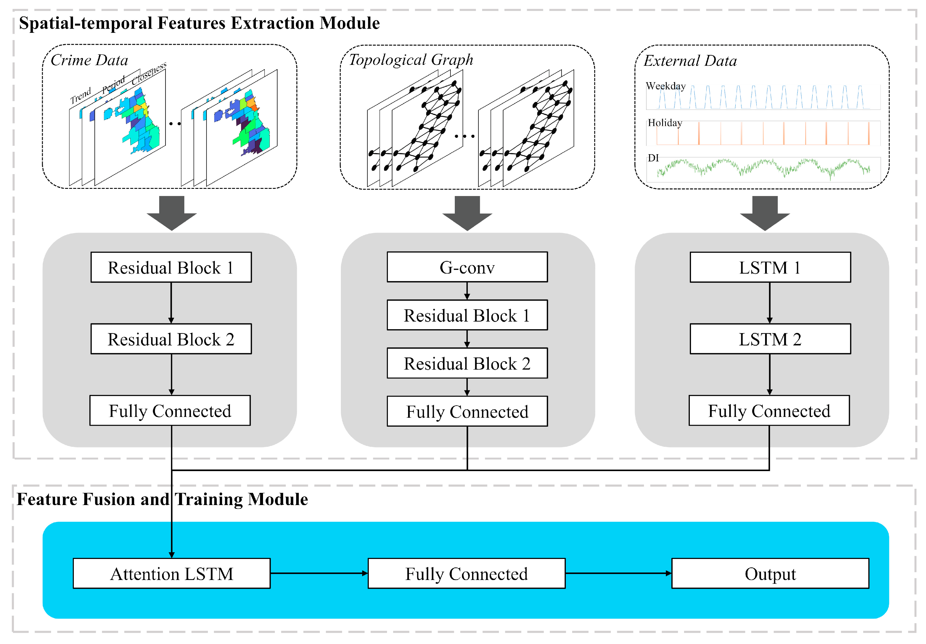
2.2. Model Framework

In this study, an integrated graph model based on attention mechanism was developed for spatial–temporal crime prediction that can extract the spatial–temporal features of crime incidents numbers and combine them with the external features. The architecture of the proposed model is presented in Figure 5. The model consisted of two modules: (i) the spatial–temporal features extraction module and (ii) the feature fusion and training module. In the feature extraction module, the spatial–temporal features of crimes, the topological features of the police districts, and the external features, such as “DI”, “Holiday”, etc., were extracted from the data. In the feature fusion and training module, all of the features were integrated into the LSTM attention to constitute a well-trained model. Finally, the test data set was employed to evaluate the prediction performance of the model, and the results were compared with those of other algorithms by using the same test set.

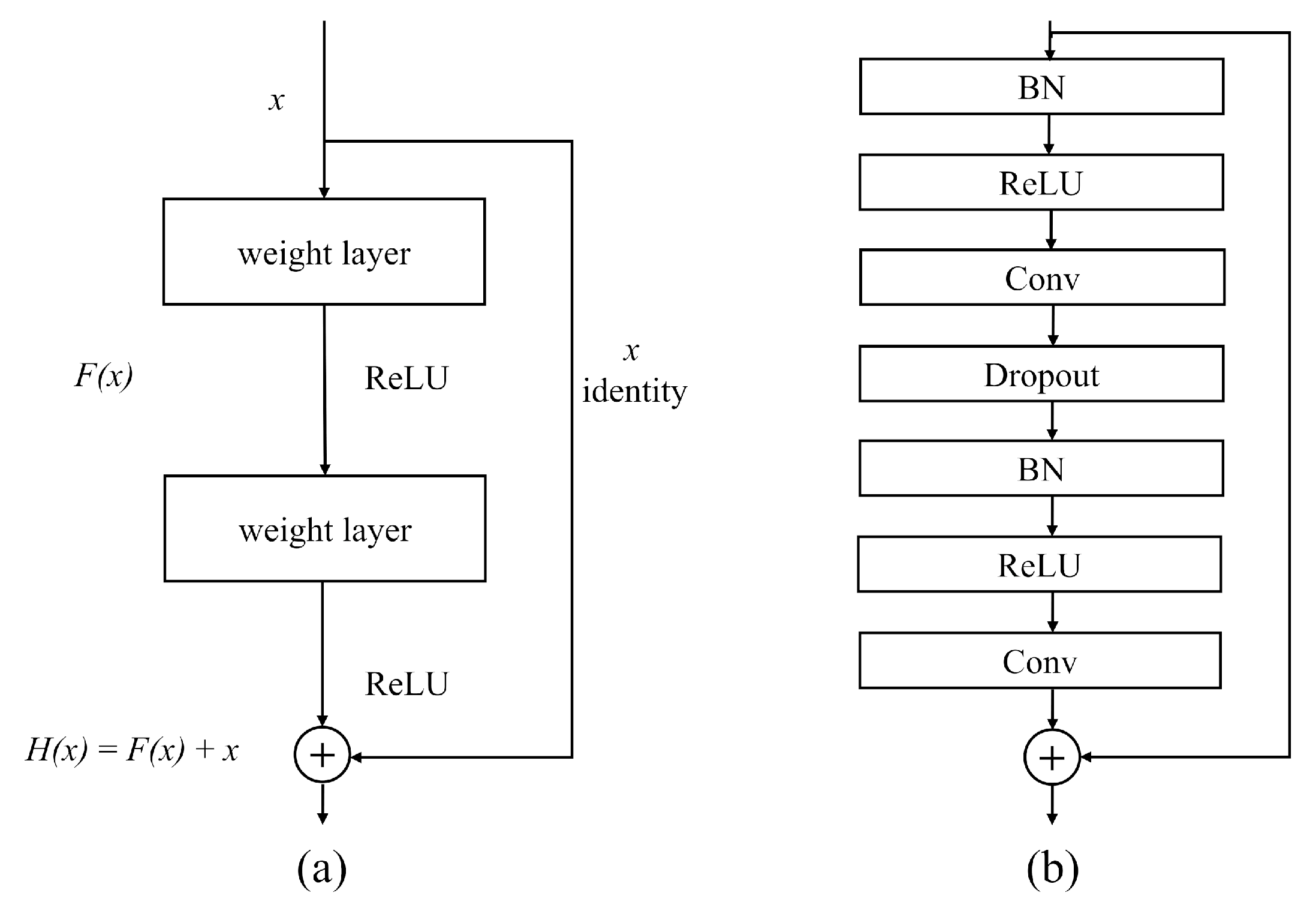
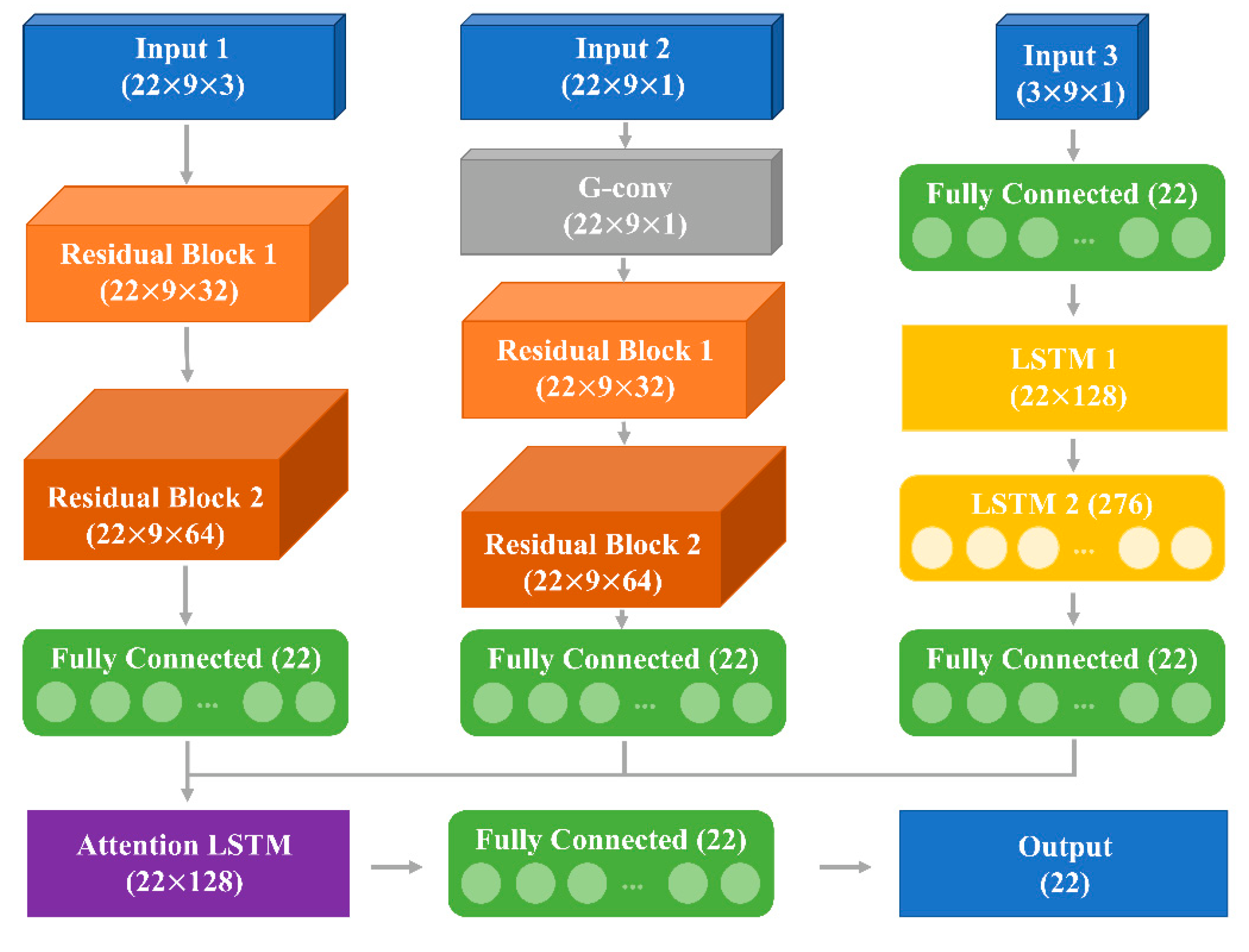
2.2.1. Spatial–Temporal Features Extraction Module

To establish the spatial–temporal features extraction module, deep residual neural networks (ResNet) were employed. ResNet was first proposed in 2015 by He et al. [30] to solve gradient disappearance, gradient explosion, network degradation, and other tricky problems induced by increasing the number of layers in convolutional neural network (CNN). ResNet is a stack of “residual blocks” as shown in Figure 6. As shown in panel (a), x represents the residual block input, F(x) + x represents the output, weight layer is a convolution layer, and rectified linear unit (ReLU) represents an activation layer [31].
In this study, an improved residual block was adopted to enhance the training speed and also the accuracy, which is illustrated in the right panel of Figure 6 [32]. The improved residual block adjusts the batch normalization (BN) and ReLU to the front of the convolutional layer (Conv). BN is used for data standardization, which can significantly accelerate the convergence of network training. By inputting the processed data into ReLU for activation, the sparsity of the network and the nonlinear relationship between layers can be enhanced; meanwhile, the impact of the overfitting problem can be alleviated. The activated data were converted to the Conv layer for feature extraction. By adding a dropout layer between Conv layers, the probability of network overfitting can be reduced. Moreover, three major features were designed to capture the spatial–temporal properties from the crime data, including closeness features, periodic features, and trend features [17,20,26,33]. Specifically, to predict the crime pattern on a certain day, the number of daily crime incidents three days before was extracted as the closeness features. The number of daily crime incidents on the 7th day, the 14th day, and the 21st day before the day was extracted as the periodic features, and the number of daily crime incidents on the corresponding dates in the past three years was extracted as the trend features. The abovementioned crime data were input into two improved residual units, and a full connection layer was used to connect with the next module.
Crime incidents in a specific district are not only temporally associated with the number of crime incidents in the past but also spatially impacted by its surrounding districts. In this study, graph convolutional network was applied to capture the network topology dependency and describe the spatial correlation of crimes more accurately [34]. The forward propagation of GCN is calculated as follows:
f ( X , A ) = ReLU ( D ˜ 1 2 A ˜ D ˜ 1 2 X W + b )
where X is the feature matrix, A is the adjacency matrix of the graph, A ˜ = A + I is the adjacency matrix with self-circulation added, D is the degree matrix, and W and b are the weight matrix and the bias, respectively [35,36,37]. In this paper, ResNet was selected as the carrier of GCN to build the network, and the topological features were input into the GCN layer and two improved residual units. Moreover, a full connection layer was used to connect the feature fusion module. As for external features, the processed data were input into two LSTM layers, and a full connection layer was also used to transmit the results into the next module.

2.2.2. Feature Fusion and Training Module

Compared with the traditional recurrent neural network (RNN) model, LSTM adds memory units to each hidden layer neural unit to obtain the controllable memory information on the time series [38,39,40]. However, when coping with enormous multi-dimensional and multivariable data, the model of LSTM may ignore some vital time-series information in practical use, resulting in poor performance. Therefore, we adopted the attention mechanism based on LSTM to fuse the features. This method can break the limitation of the encode–decoder architecture and the fixed-length internal representation. The attention mechanism can be used to simulate the attention mechanism of human brains [41,42]. Attention LSTM retains the intermediate states of the LSTM encoder and selectively learns these intermediate states through the training model. The LSTM model can be combined with the attention mechanism to give different weights to the input characteristics of the LSTM and highlight the critical influencing features without increasing the calculation and storage overhead of the model, helping LSTM to make more accurate judgment [43]. Let matrix XRm × n be the LSTM output, where m is the timesteps, and n represents the number of features in each timestep. Then, the mathematical formulation of the attention-based output (OAttention) is presented as follows:
A = f ( W X + b )
O Attention = A X
where A is a weight matrix with the same shape as X, “ ” represents the Hadamard product, f represents the fully connected layer, and W and b denote the weight matrix and the bias, respectively [44]. In this module, feature fusion was completed through the weighted calculation of multiple features. The spatial prediction module and the temporal prediction module were not separated in the proposed model. Thus, the “offline” problem was solved as well. The results from the spatial–temporal features extraction module were input into the attention LSTM, which was followed by another fully connected layer to output the final results.

2.3. Case Study

2.3.1. Model Configuration

The proposed model was implemented by Keras and TensorFlow. The system hardware of the server we used included a CPU with two cores (Intel Xeon E5 Core *20), four GPUs (Nvidia Tesla P100 16GB), four memory modules (Kingston 64GB 2666MHz), and three hard disks (4TB). Both theft and assault incidents data from 1 January 2015 to 31 December 2019 were used to train this model, and the incident data from 1 January to 7 January 2020 were used as the test set. The validation split rate was set as 0.2 to calibrate the model. The dimensions of tensors flowing in the proposed model are shown in Figure 7. In terms of the crime data processing part, the first residual block in the spatial–temporal features extraction module had 32 filters, whereas the second one had 64 filters. The kernel size was 3 × 3 and the fully connected layer consisted of 22 neurons. The topological features processing part passed through a GCN layer first, and then the remaining configuration was the same as the crime data processing part. Two residual blocks had 32 and 64 filters, respectively. The kernel size was 3 × 3 and the fully connected layer consisted of 22 neurons in that case. As for the external data processing part, the two LSTM layers consisted of 128 and 276 neurons, respectively, and the fully connected layers comprised 22 neurons. For feature fusion and training module, the attention LSTM and final fully connected layers consisted of 128 and 22 neurons, respectively. Furthermore, we adopted end-to-end training to optimize the model. The mean squared error (MSE) was used as the loss function. The optimizer was “NAdam”, with a learning rate of 0.001.

2.3.2. Baseline Models

In this study, eight algorithms were compared with our model to verify its performance, including ARMIA [45], ridge regression [46], support vector regression (SVR) [47], random forest [48], XGBoost [49], LSTM [50], CNN [51], and Conv-LSTM [52]. The specific configurations are shown in Table 2.

2.4. Evaluation Metrics

To evaluate the prediction performance of the proposed model, MAE and RMSE were utilized as evaluation metrics. The mathematical formulation of MAE and RMSE is as follows:
MAE = 1 n i = 1 n | Y i Y ^ i |
RMSE = 1 n i = 1 n ( Y i Y ^ i ) 2
where Y i is the observed value, Y ^ i is the predicted value, and n is the prediction sample numbers. Smaller value of MAE and RMSE indicates higher prediction accuracy of the model [53,54]. In this study, nine prediction models were trained and tested based on the same data set.

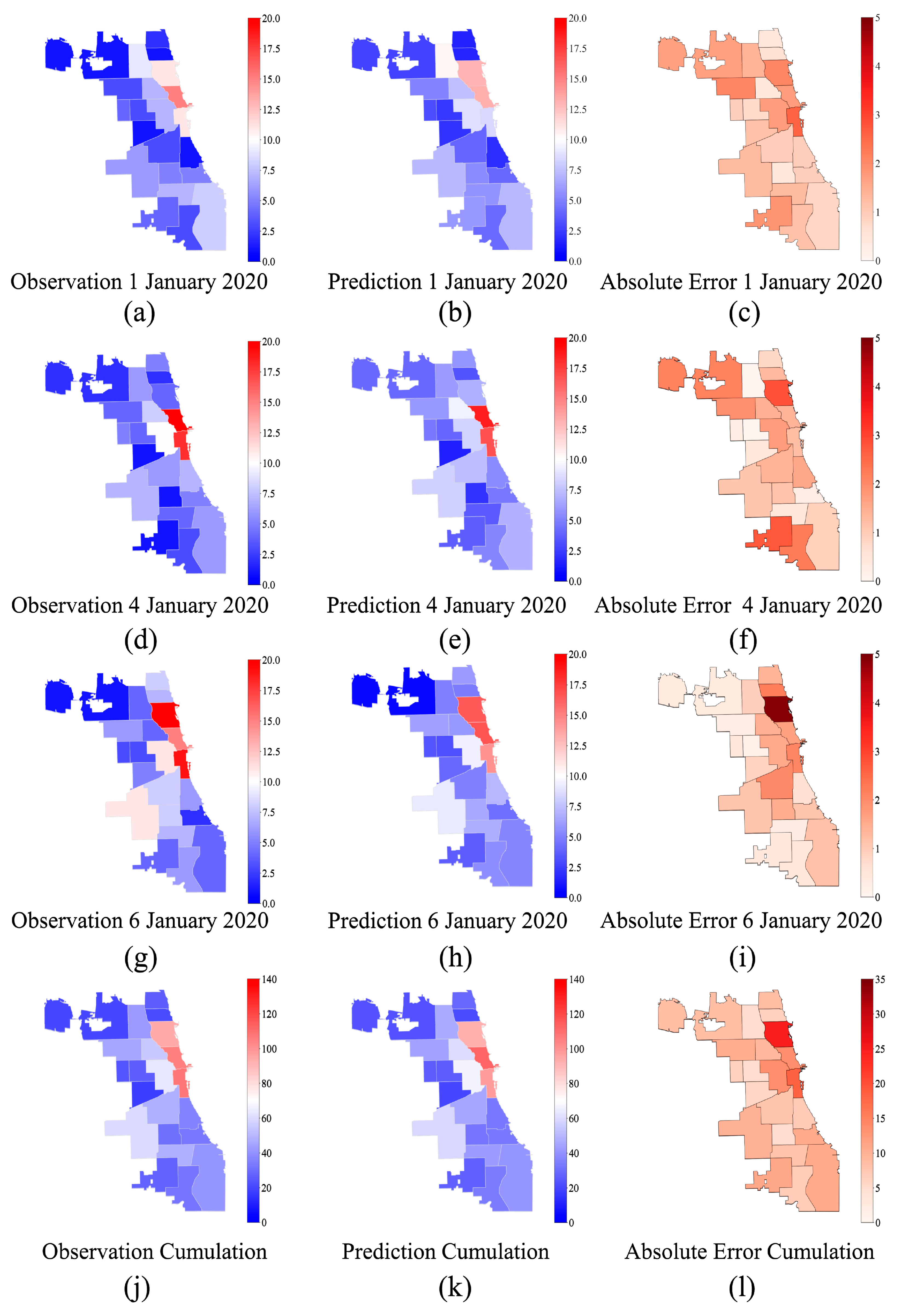
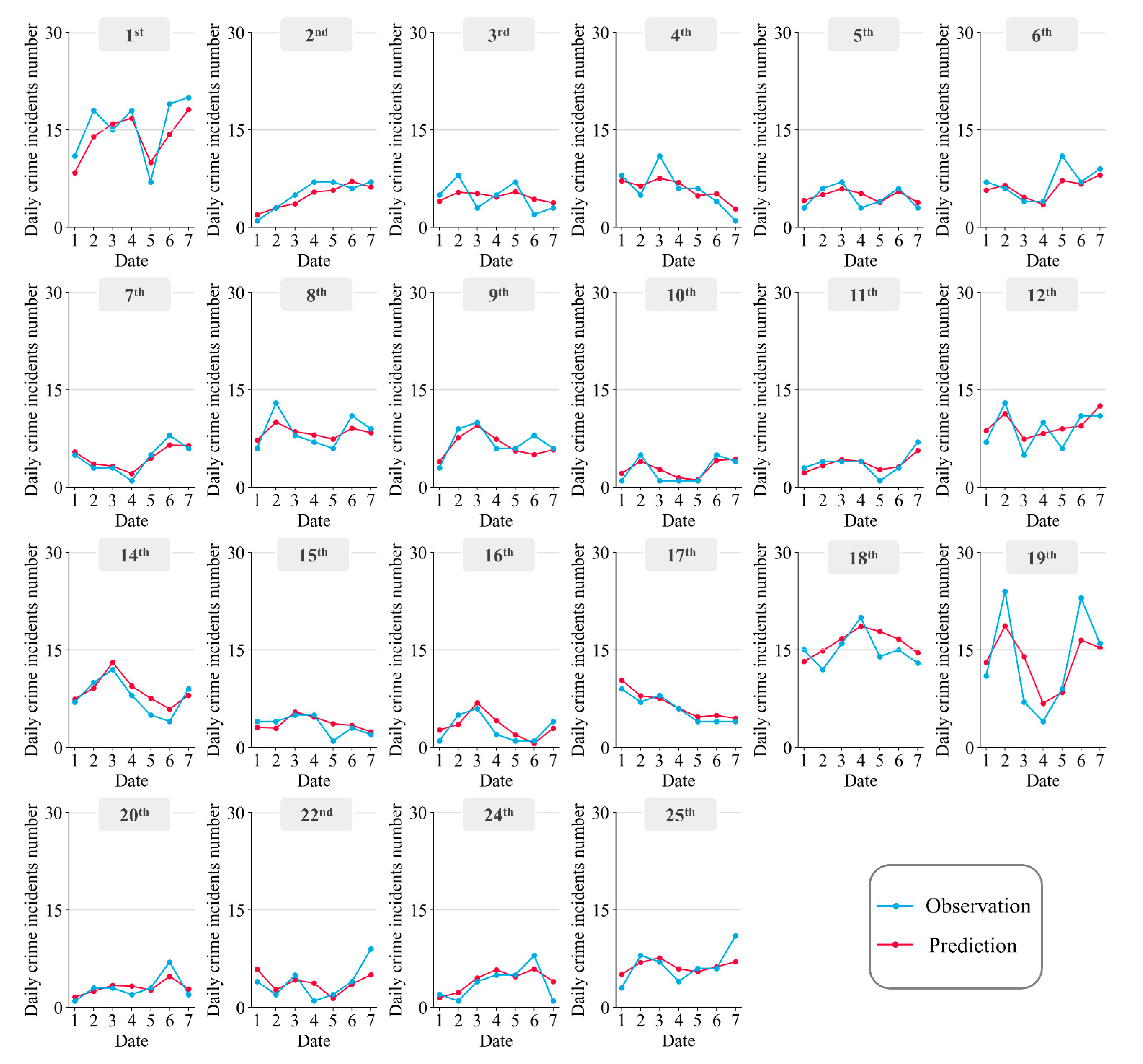
3. Results and Discussion

To analyze the experimental results and evaluate the performance of the proposed model, data in the 22 police districts from 1 January 2020, to 7 January 2020 (7 days) were selected to build the test set. Figure 8 (for theft) and Figure 9 (for assault) show the spatial patterns of the observed crime incidents, prediction of crime incidents numbers, and absolute error (AE) in three representative days (namely 1, 4, and 6 January 2020), as well as the cumulative values from 1 to 7 January 2020. Among the three selected days, 1 January 2020 is a holiday, 4 January 2020 is a weekday, and 6 January 2020 is a weekend.
As shown in Figure 8, the predicted patterns of theft are very close to the real distributions, and, as shown in the maps, the proposed model accurately captures the spatial hot areas of theft, not only on the selected three days but also for the cumulated results. Specifically, on 1 January 2020, the 1st district has the max AE (2.57) among the 22 police districts. As for 4 January 2020 and 6 January 2020, the 19th district witnesses the max AE of 2.80 and 4.87, respectively. Moreover, the 19th district also has the max AE (24.81) for the cumulative values. In terms of the 22 police districts, the average AE on 1 January 2020, 4 January 2020, 6 January 2020, and the cumulations of seven days are 1.24, 1.24, 1.22, and 9.63, which indicates that the proposed model has reliable accuracy in this experiment. The spatial patterns of theft show that the 1st district and the 19th district have larger absolute errors than others. As investigated, both the above two districts are in the northeast of Chicago, which are the main tourist attractions, with many downtown areas of this city. Thus, it is one of the most crowded areas and is usually reported as a hotspot of theft, so various factors, such as the population density, unemployment rate, traffic condition, etc., may comprehensively influence the crime rates, which increase the difficulty in accurately forecasting the daily theft numbers in these districts.
With regard to assault, Figure 9 reports that the predicted spatial–temporal patterns on the test set have close agreements with the observations. Specifically, the spatial hot areas of assault are captured by the proposed prediction model in terms of the cumulative values. Error distributions in the right panels of Figure 9 points out that the 15th district witnesses the max AE (2.31) among the 22 police districts on 1 January 2020, the 8th district has the max AE (1.84) on 4 January 2020, and the 7th district has the max AE of 2.21 on 6 January 2020. The spatial average AE on 1, 4, and 6 January are 0.88, 0.71, and 0.65, proving that this model can accurately forecast the spatial pattern of assault, with an average error lower than one incident. As for the spatial patterns of assault, the police districts with large absolute errors are mainly in the southwest of Chicago, especially the 7th district. The 7th district has a lot of violent incidents due to its complicated ethnic composition and extreme disparity in income. Therefore, the reason why the AE in the 7th district is larger than other places may be that a variety of social factors are associated with crimes, which adds more uncertainty to the prediction of crimes.
Figure 10 and Figure 11 show the prediction of theft and assault incidents numbers of the 22 police districts in Chicago, respectively. As shown in Figure 10 and Figure 11, the predicted value is quite close to the actual value in terms of both theft and assault. Though heavy fluctuations are observed in theft incidents in the 1st, 18th, and 19th districts and in assault incidents in the 4th, 7th, and 22nd districts, this model can also predict the temporal trends with limited errors. Thus, from these two figures, we can find that the temporal patterns of both theft and assault are accurately predicted on the test set, showing a reliable performance of this integrated graph model.
In order to quantitatively examine the overall performance of this model, evaluation metrics (MAE and RMSE) were used. The MAE and RMSE of ARIMA, ridge regression, SVR, random forest, XGBoost, LSTM, CNN, and Conv-LSTM were also calculated as comparisons. In the comparative experiments, the same dataset and the extracted features were used among all of the models. The obtained results are shown in Table 3. The average values of the indices are lower than two incidents for theft (MAE = 1.3778, RMSE =1.6318) and one incident for assault (MAE = 0.7457, RMSE =0.8851), which indicates that this model has a good performance in spatial–temporal crime prediction. Compared with other models, the proposed model has a better performance in terms of both MAE and RMSE since the second lowest MAE (RMSE) of theft is 1.5574 (1.8736) from Conv-LSTM, whereas that of assault is 0.8269 (0.9863), which is also from Conv-LSTM. In addition, the results in this table also point out that the performance of ARIMA, ridge regression, SVR, random forest, or XGBoost is significantly worse than the deep learning models LSTM, CNN, and Conv-LSTM. The reason may be that it is difficult for SVR (and the other statistics-based and traditional machine learning models) to capture the complex features from the spatial–temporal crime data. For the deep learning models, the performance of LSTM is considerably worse than CNN and Conv-LSTM. As is known, the latter two are good at exploring the spatial autocorrelation of the variables and extracting advanced features of the daily spatial distributions of crimes. Since spatial information usually plays an important role in spatial–temporal crime prediction, CNN and Conv-LSTM are better suited to this scenario than original LSTM, which is only able to examine the temporal patterns. Interestingly, the integrated graph model proposed in this study has a much better performance than the three other deep learning models. The reason may be that the three other deep learning models are based on regular spatial–temporal grids for spatial division. However, many latent spatial correlations among the real administrative districts (such as the policing districts) cannot be well captured, which may adversely affect the prediction performance of such models. By contrast, the proposed model extracts the topological relationships of the 22 police districts in the city using ResNet and GCN. The attention mechanism is also investigated to fuse the complicated features through the weighted calculations. This indicates that the integrated graph model is a practical and effective solution for spatial–temporal crime prediction and it is also convenient and feasible with respect to practical applications.

4. Conclusions

In this study, an “online” integrated graph model based on an attention mechanism is proposed to predict the urban spatial–temporal crime patterns at a daily scale. This integrated graph model combines ResNet, GCN, and LSTM with the attention mechanism to extract and fuse the spatial–temporal features, topological graphs, and external features from the data of crime incidents. To validate this model, the daily theft and assault data at a police-district-scale of the city of Chicago in the US from 1 January 2015 to 7 January 2020 were employed. Indices MAE and RMSE were conducted to quantitatively evaluate this model, as well as eight other models (which were used as the comparisons) proposed in previous studies. The main findings of this study are summarized as follows:
(1) The predicted spatial–temporal patterns by using the proposed model have close agreements with the observations. Meanwhile, the average values of the two metrics (MAE and RMSE) are lower than two incidents for theft and one incident for assault, which indicates that this model achieves an extraordinarily high accuracy for predicting the spatial–temporal crime patterns. Moreover, the proposed model has a much better performance than all of the other eight models in terms of both MAE and RMSE. These results indicate that the integrated graph model can effectively predict the urban spatial–temporal distribution of crimes at a daily scale.
(2) This prediction method adopts irregular divisions on urban districts so that crime incident numbers in different police districts can be predicted. In addition, feature fusion is achieved by weighting the features through the attention mechanism, which provides an “online” framework to support the decision making for police, including patrolling and investigation, as well as other police resource allocation works.
The performance of this integrated graph model still has room for improvement. Our experimental results indicate that the prediction accuracy of this model would be lower in the districts where complicated social factors are aggregated. If more real-time and police-district-scale data, such as the house price, population density, traffic condition, and unemployment rate, are included in the future research, the performance of this model is expected to be further improved.

Author Contributions

Conceptualization, Xiaofeng Hu; methodology, Xiaofeng Hu, Miaomiao Hou, Xinge Han, Jitao Cai and Shuaiqi Yuan; validation, Xiaofeng Hu and Miaomiao Hou; formal analysis, Xiaofeng Hu and Miaomiao Hou; investigation, Xiaofeng Hu and Miaomiao Hou; resources, Xiaofeng Hu and Miaomiao Hou; data curation, Miaomiao Hou; writing—original draft preparation, Miaomiao Hou; writing—review and editing, Xiaofeng Hu, Miaomiao Hou, and Jitao Cai; visualization, Miaomiao Hou; supervision, Xiaofeng Hu; project administration, Xiaofeng Hu; funding acquisition, Xiaofeng Hu. All authors have read and agreed to the published version of the manuscript.

Funding

This research was funded by the National Natural Science Foundation of China (Grant No. 72174203).

Data Availability Statement

The data that support the findings of this study are available from the Chicago open data portal (https://data.cityofchicago.org/, accessed on 1 October 2020) and rp5 website (http://rp5.ru/, accessed on 1 October 2020).

Acknowledgments

We thank the anonymous reviewers and academic editor for the constructive suggestions and insightful comments that substantially improved the quality of this research.

Conflicts of Interest

The authors declare no conflict of interest.

Appendix A

Table A1. The descriptive statistics of theft and assault incidents numbers in the 22 police districts of Chicago from 1 January 2015 to 7 January 2020.
Police
District
TheftAssault
MeanStandard deviationMinMaxSumMeanStandard deviationMinMaxSum
1st District18.7547.397310834,3761.9391.472093554
2nd District7.1953.04501913,1882.4831.6810104552
3rd District5.3502.47201598063.0111.798095519
4th District6.3182.87002711,5803.7271.9860116831
5th District4.8012.32701488012.8831.8250125285
6th District8.1783.17202614,9913.9822.1300127299
7th District5.1602.49701594583.5522.0360126510
8th District9.0743.46102416,6323.3602.0050116158
9th District6.1552.79801811,2832.5911.7020104750
10th District4.7852.43301587712.5861.6830104741
11th District5.4472.51401599853.5942.0250136588
12th District11.4754.37713321,0342.3371.6670104283
14th District9.3623.77502517,1601.4601.268072676
15th District3.6622.10201467122.3461.583094300
16th District5.7612.81402010,5591.6491.320083023
17th District5.7062.70301610,4591.1991.133062197
18th District18.0436.32334233,0721.5181.320092782
19th District11.8904.44214721,7951.5361.251072815
20th District3.3992.02101262310.8030.903051472
22nd District4.6872.47001785921.7831.349073269
24th District5.4512.67401799911.3621.215072497
25th District7.3892.99801813,5442.8091.7510115148
Total168.04128.18761309308,02052.50910.937238896,249

Appendix B

The discomfort index (DI) is in line with the description of the human body temperature perception, which can be calculated according to temperature, humidity, and wind speed as follows:
DI = 0.5 T w + 0.5 A T
A T = 1.07 T + 0.2 e 0.65 v 2.7
e = ( R H ÷ 100 ) × 6.105 × e 17.2 T 237.7 + T
T w = A T arctan ( 0.152 R H + 8.314 ) + arctan ( A T + R H ) arctan ( R H 1.676 ) + 0.0039 R H 3 2 arctan ( 0.023 R H ) 4.6803
where AT is the apparent temperature (°C), TW is the thermodynamic wet-bulb temperature (°C), T is the air temperature (°C), e is the water vapor pressure (hPa), V is the wind speed (m/s), and RH is relative humidity (%). Weather data used to calculate DI in Chicago are obtained from the rp5 website (http://rp5.ru/, accessed on 1 October 2020).

References

  1. Rummens, A.; Hardyns, W.; Pauwels, L. The use of predictive analysis in spatiotemporal crime forecasting: Building and testing a model in an urban context. Appl. Geogr. 2017, 86, 255–261. [Google Scholar] [CrossRef]
  2. Kwon, E.; Jung, S.; Lee, J. Artificial Neural Network Model Development to Predict Theft Types in Consideration of Environmental Factors. ISPRS Int. J. Geo-Inf. 2021, 10, 99. [Google Scholar] [CrossRef]
  3. Sherman, L.W.; Gartin, P.R.; Buerger, M.E. Hot spots of predatory crime: Routine activities and the criminology of place. Criminology 1989, 27, 27–56. [Google Scholar] [CrossRef]
  4. He, Z.; Tao, L.; Xie, Z.; Xu, C. Discovering spatial interaction patterns of near repeat crime by spatial association rules mining. Sci. Rep. 2020, 10, 17262. [Google Scholar] [CrossRef]
  5. Gu, H.; Chen, P.; Li, H. Review and prospect of the research on the methods of crime space-time prediction. J. Earth Inf. Sci. 2021, 23, 43–57. [Google Scholar]
  6. Lamari, Y.; Freskura, B.; Abdessamad, A.; Eichberg, S.; de Bonviller, S. Predicting Spatial Crime Occurrences through an Efficient Ensemble-Learning Model. ISPRS Int. J. Geo-Inf. 2020, 9, 645. [Google Scholar] [CrossRef]
  7. Marques, S.C.; Ferreira, F.A.; Meidutė-Kavaliauskienė, I.; Banaitis, A. Classifying urban residential areas based on their exposure to crime: A constructivist approach. Sustain. Cities Soc. 2018, 39, 418–429. [Google Scholar] [CrossRef]
  8. Maiti, A.; Zhang, Q.; Sannigrahi, S.; Pramanik, S.; Chakraborti, S.; Cerda, A.; Pilla, F. Exploring spatiotemporal effects of the driving factors on COVID-19 incidences in the contiguous United States. Sustain. Cities Soc. 2021, 68, 102784. [Google Scholar] [CrossRef]
  9. Ingilevich, V.; Ivanov, S. Crime rate prediction in the urban environment using social factors. Procedia Comput. Sci. 2018, 136, 472–478. [Google Scholar] [CrossRef]
  10. Yu, H.; Liu, L.; Yang, B.; Lan, M. Crime Prediction with Historical Crime and Movement Data of Potential Offenders Using a Spatio-Temporal Cokriging Method. ISPRS Int. J. Geo-Inf. 2020, 9, 732. [Google Scholar] [CrossRef]
  11. Dash, S.K.; Safro, I.; Srinivasamurthy, R.S. Spatio-temporal prediction of crimes using network analytic approach. In Proceedings of the 2018 IEEE International Conference on Big Data (Big Data), Seattle, WA, USA, 10–13 December 2018; pp. 1912–1917. [Google Scholar]
  12. Chen, P.; Hu, X.; Chen, J. The application of fuzzy information granulation and support vector machine in crime forecasting. Sci. Technol. Eng. 2015, 35, 54–57. [Google Scholar]
  13. Pillai, R. Optimized Predictive Modelling to Unfold the Links of Crime with Education, Safety and Climate in Chicago; National College of Ireland: Dublin, Ireland, 2019. [Google Scholar]
  14. LeCun, Y.; Bengio, Y. Convolutional networks for images, speech, and time series. Handb. Brain Theory Neural Netw. 1995, 3361, 1995. [Google Scholar]
  15. Cheng, T.; Wang, J. Application of a dynamic recurrent neural network in spatio-temporal forecasting. In Information Fusion and Geographic Information Systems; Springer: St. Petersburg, Russia, 2007; pp. 173–186. [Google Scholar]
  16. Li, W.; Wen, L.; Chen, Y. Spatial—Temporal forecast research of property crime under the driven of urban traffic factors. Multimed. Tools Appl. 2016, 75, 17669–17687. [Google Scholar]
  17. Zhang, H.; Zhang, J.; Wang, Z.; Yin, H. An Adaptive Spatial Resolution Method Based on the ST-ResNet Model for Hourly Property Crime Prediction. ISPRS Int. J. Geo-Inf. 2021, 10, 314. [Google Scholar] [CrossRef]
  18. Qian, Y.; Pan, L.; Wu, P.; Xia, Z. GeST: A Grid Embedding based Spatio-Temporal Correlation Model for Crime Prediction. In Proceedings of the 2020 IEEE Fifth International Conference on Data Science in Cyberspace (DSC), Hong Kong, China, 27–30 July 2020; pp. 1–7. [Google Scholar]
  19. Zhang, T.; Ran, Y.; Wei, D. Application of Grid Management in Spatio-temporal Prediction of Crime. In Proceedings of the 2021 33rd Chinese Control and Decision Conference (CCDC), Kunming, China, 22–24 May 2021; pp. 2745–2749. [Google Scholar]
  20. Han, X.; Hu, X.; Wu, H.; Shen, B.; Wu, J. Risk Prediction of Theft Crimes in Urban Communities: An Integrated Model of LSTM and ST-GCN. IEEE Access 2020, 8, 217222–217230. [Google Scholar] [CrossRef]
  21. Hu, T.; Zhu, X.; Duan, L.; Guo, W. Urban crime prediction based on spatio-temporal Bayesian model. PLoS ONE 2018, 13, e0206215. [Google Scholar] [CrossRef] [PubMed]
  22. Yi, F.; Yu, Z.; Zhuang, F.; Zhang, X.; Xiong, H. An integrated model for crime prediction using temporal and spatial factors. In Proceedings of the 2018 IEEE International Conference on Data Mining (ICDM), Singapore, 17–20 November 2018; pp. 1386–1391. [Google Scholar]
  23. Sun, J.; Yue, M.; Lin, Z.; Yang, X.; Nocera, L.; Kahn, G.; Shahabi, C. CrimeForecaster: Crime Prediction by Exploiting the Geographical Neighborhoods’ Spatiotemporal Dependencies. In Proceedings of the Joint European Conference on Machine Learning and Knowledge Discovery in Databases, Ghent, Belgium, 14–18 September 2020; pp. 52–67. [Google Scholar]
  24. Chen, X.; Cho, Y.; Jang, S.Y. Crime prediction using Twitter sentiment and weather. In Proceedings of the 2015 Systems and Information Engineering Design Symposium, Charlottesville, VA, USA, 24–24 April 2015; pp. 63–68. [Google Scholar]
  25. Zhao, X.; Tang, J. Modeling temporal-spatial correlations for crime prediction. In Proceedings of the 2017 ACM on Conference on Information and Knowledge Management, Singapore, 6–10 November 2017; pp. 497–506. [Google Scholar]
  26. Wang, B.; Yin, P.; Bertozzi, A.L.; Brantingham, P.J.; Osher, S.J.; Xin, J. Deep learning for real-time crime forecasting and its ternarization. Chin. Ann. Math. Ser. B 2019, 40, 949–966. [Google Scholar] [CrossRef] [Green Version]
  27. Hu, X.; Chen, P.; Huang, H.; Sun, T.; Li, D. Contrasting impacts of heat stress on violent and nonviolent robbery in Beijing, China. Nat. Hazards 2017, 87, 961–972. [Google Scholar] [CrossRef]
  28. Hu, X.; Wu, J.; Chen, P.; Sun, T.; Li, D. Impact of climate variability and change on crime rates in Tangshan, China. Sci. Total Environ. 2017, 609, 1041–1048. [Google Scholar] [CrossRef] [Green Version]
  29. Xu, R.; Xiong, X.; Abramson, M.J.; Li, S.; Guo, Y. Association between ambient temperature and sex offense: A case-crossover study in seven large US cities, 2007–2017. Sustain. Cities Soc. 2021, 69, 102828. [Google Scholar] [CrossRef]
  30. He, K.; Zhang, X.; Ren, S.; Sun, J. Deep residual learning for image recognition. In Proceedings of the IEEE Conference on Computer Vision and Pattern Recognition, Las Vegas, NV, USA, 27–30 June 2016; pp. 770–778. [Google Scholar]
  31. Loey, M.; Manogaran, G.; Taha, M.H.N.; Khalifa, N.E.M. Fighting against COVID-19: A novel deep learning model based on YOLO-v2 with ResNet-50 for medical face mask detection. Sustain. Cities Soc. 2021, 65, 102600. [Google Scholar] [CrossRef] [PubMed]
  32. He, K.; Zhang, X.; Ren, S.; Sun, J. Identity mappings in deep residual networks. In Proceedings of the European Conference on Computer Vision, Amsterdam, The Netherlands, 11–14 October 2016; pp. 630–645. [Google Scholar]
  33. Wang, B.; Zhang, D.; Zhang, D.; Brantingham, P.J.; Bertozzi, A.L. Deep learning for real time crime forecasting. arXiv 2017, arXiv:1707.03340. [Google Scholar]
  34. Lu, L.; Lyu, B. Reducing energy consumption of Neural Architecture Search: An inference latency prediction framework. Sustain. Cities Soc. 2021, 67, 102747. [Google Scholar] [CrossRef]
  35. Wang, Y.; Jing, C. Spatiotemporal Graph Convolutional Network for Multi-Scale Traffic Forecasting. ISPRS Int. J. Geo-Inf. 2022, 11, 102. [Google Scholar] [CrossRef]
  36. Bai, J.; Zhu, J.; Song, Y.; Zhao, L.; Hou, Z.; Du, R.; Li, H. A3t-gcn: Attention temporal graph convolutional network for traffic forecasting. ISPRS Int. J. Geo-Inf. 2021, 10, 485. [Google Scholar] [CrossRef]
  37. Zhang, J.; Chen, F.; Guo, Y.; Li, X. Multi-graph convolutional network for short-term passenger flow forecasting in urban rail transit. IET Intell. Transp. Syst. 2020, 14, 1210–1217. [Google Scholar] [CrossRef]
  38. Ma, X.; Tao, Z.; Wang, Y.; Yu, H.; Wang, Y. Long short-term memory neural network for traffic speed prediction using remote microwave sensor data. Transp. Res. Part C Emerg. Technol. 2015, 54, 187–197. [Google Scholar] [CrossRef]
  39. Yan, J.; Hou, M. Predicting Time Series of Theft Crimes Based on LSTM Network. Data Anal. Knowl. Discov. 2020, 4, 84–91. [Google Scholar]
  40. Mao, W.; Wang, W.; Jiao, L.; Zhao, S.; Liu, A. Modeling air quality prediction using a deep learning approach: Method optimization and evaluation. Sustain. Cities Soc. 2021, 65, 102567. [Google Scholar] [CrossRef]
  41. Treisman, A.M.; Gelade, G. A feature-integration theory of attention. Cogn. Psychol. 1980, 12, 97–136. [Google Scholar] [CrossRef]
  42. Li, Y.; Tong, Z.; Tong, S.; Westerdahl, D. A data-driven interval forecasting model for building energy prediction using attention-based LSTM and fuzzy information granulation. Sustain. Cities Soc. 2022, 76, 103481. [Google Scholar] [CrossRef]
  43. Li, Y.; Zhu, Z.; Kong, D.; Han, H.; Zhao, Y. EA-LSTM: Evolutionary attention-based LSTM for time series prediction. Knowl. Based Syst. 2019, 181, 104785. [Google Scholar] [CrossRef] [Green Version]
  44. Kim, S.; Kang, M. Financial series prediction using Attention LSTM. arXiv 2019, arXiv:1902.10877. [Google Scholar]
  45. Box, G.E.; Pierce, D.A. Distribution of residual autocorrelations in autoregressive-integrated moving average time series models. J. Am. Stat. Assoc. 1970, 65, 1509–1526. [Google Scholar] [CrossRef]
  46. Hoerl, A.E.; Kennard, R.W. Ridge regression: Biased estimation for nonorthogonal problems. Technometrics 1970, 12, 55–67. [Google Scholar] [CrossRef]
  47. Awad, M.; Khanna, R. Support vector regression. In Efficient Learning Machines; Springer: Berkeley, CA, USA, 2015; pp. 67–80. [Google Scholar]
  48. Alves, L.G.; Ribeiro, H.V.; Rodrigues, F.A. Crime prediction through urban metrics and statistical learning. Phys. A Stat. Mech. Its Appl. 2018, 505, 435–443. [Google Scholar] [CrossRef] [Green Version]
  49. Chen, T.; He, T.; Benesty, M.; Khotilovich, V.; Tang, Y.; Cho, H. Xgboost: Extreme gradient boosting. R Package Version 0.4-2 2015, 1, 1–4. [Google Scholar]
  50. Cortez, B.; Carrera, B.; Kim, Y.-J.; Jung, J.-Y. An architecture for emergency event prediction using LSTM recurrent neural networks. Expert Syst. Appl. 2018, 97, 315–324. [Google Scholar] [CrossRef]
  51. Duan, L.; Hu, T.; Cheng, E.; Zhu, J.; Gao, C. Deep convolutional neural networks for spatiotemporal crime prediction. In Proceedings of the International Conference on Information and Knowledge Engineering (IKE), Monte Carlo Resort, Las Vegas, NV, USA, 17–20 July 2017; pp. 61–67. [Google Scholar]
  52. Shi, X.; Chen, Z.; Wang, H.; Yeung, D.-Y.; Wong, W.-K.; Woo, W.-C. Convolutional LSTM network: A machine learning approach for precipitation nowcasting. In Proceedings of the Advances in Neural Information Processing Systems, Montreal, QC, Canada, 7–12 December 2015; pp. 802–810. [Google Scholar]
  53. Willmott, C.J.; Matsuura, K. Advantages of the mean absolute error (MAE) over the root mean square error (RMSE) in assessing average model performance. Clim. Res. 2005, 30, 79–82. [Google Scholar] [CrossRef]
  54. Shen, B.; Hu, X.; Wu, H. Impacts of climate variations on crime rates in Beijing, China. Sci. Total Environ. 2020, 725, 138190. [Google Scholar] [CrossRef]
Figure 1. Map of the police districts in Chicago.
Ijgi 11 00294 g001
Figure 2. Daily number of theft and assault incidents in the 22 police districts of Chicago from 1 January 2015, to 7 January 2020. Blue line and green line represent theft and assault incidents numbers, respectively.
Ijgi 11 00294 g002
Figure 3. The spatial patterns of theft and assault incidents numbers in the 22 police districts of Chicago from 1 January 2015, to 7 January 2020. Panel (a) shows the distribution of theft incidents numbers, whereas panel (b) is the spatial pattern of assault.
Ijgi 11 00294 g003
Figure 4. The administrative map and topological map of the 22 police districts in Chicago. Panel (a) shows the administrative map, whereas panel (b) is the topological map.
Ijgi 11 00294 g004
Figure 5. The architecture of the proposed integrated graph model.
Ijgi 11 00294 g005
Figure 6. Two types of residual blocks. Panel (a) shows the original residual block, whereas panel (b) is the improved residual blocks.
Ijgi 11 00294 g006
Figure 7. Dimensions of tensors flowing in the proposed model.
Ijgi 11 00294 g007
Figure 8. Spatial patterns of the predicted theft incidents numbers of different police districts in Chicago. The left panels (a,d,g,j) show the observed crime distributions, the middle panels (b,e,h,k) represent the predicted patterns, and the right panels (c,f,i,l) are about the AE values between prediction and observation. Panels from top to bottom represent values on January 1, 4, and 6, 2020, and that of the cumulations from 1 to 7 January 2020.
Ijgi 11 00294 g008
Figure 9. Spatial patterns of the predicted assault incidents numbers of different police districts in Chicago. The left panels (a,d,g,j) show the observed crime distributions, the middle panels (b,e,h,k) represent the predicted patterns, and the right panels (c,f,i,l) are about the AE values between prediction and observation. Panels from top to bottom represent values on January 1, 4, and 6, 2020, and that of the cumulations from 1 to 7 January 2020.
Ijgi 11 00294 g009
Figure 10. The prediction of daily theft incidents numbers of the 22 police districts in Chicago. Blue lines and points represent the observed daily crime numbers, whereas red lines and points represent the predictions.
Ijgi 11 00294 g010
Figure 11. The prediction of daily assault incidents numbers of the 22 police districts in Chicago. Blue lines and points represent the observed daily crime numbers, whereas red lines and points represent the predictions.
Ijgi 11 00294 g011
Table 1. The brief descriptions of external features.
Feature NameDescription
WeekendThe feature “Weekend” represents whether the day is a weekday or a weekend.
HolidayThe feature “Holiday” represents whether the day is a holiday or not.
DIThe heat stress index DI is calculated according to temperature, humidity, and wind speed (as shown in Appendix B).
Table 2. The specific configurations of baseline models.
Baseline Models.Specific Configurations
ARIMAThe best ARIMA results are obtained automatically by Expert Modeler in the Statistical Package for the Social Sciences (SPSS) software.
Ridge RegressionThe hyperparameters of ridge regression are obtained automatically by the RidgeCV class in the scikit-learn library.
SVRThe kernel of SVR is set as a radial-basis function, the regularization parameter C is set as 1.0, and the tolerance for stopping criterion is set as 0.001.
Random ForestThe number of trees in random forest is set as 100, and the maximum tree depth is set as 10.
XGBoostThe number of iterations is set as 100, and the maximum tree depth is set as 10.
LSTMThe LSTM has two kernel layers (each containing 100 neurons), and the learning rate is set as 0.0001.
CNNThe CNN has two kernel layers, the number of filters is set as 32 and 64, the size of the kernel is set as 3 × 3, the input length is set as 12, and the learning rate is set as 0.005.
Conv-LSTMThe number of Conv-LSTM layers is set as 2 with 32 and 64 filters, respectively, the kernel size is 3 × 3, the input length is set as 12, and the learning rate is set as 0.005.
Table 3. Performances in spatial–temporal prediction of theft and assault in terms of MAE and RMSE.
ModelTheftAssault
MAERMSEMAERMSE
ARIMA3.31453.80031.75942.1025
Ridge Regression2.91683.49981.49171.9215
SVR2.80303.37111.46091.8598
Random Forest2.50642.99961.31911.5958
XGBoost2.51143.00371.32181.5818
LSTM1.83792.23951.14621.3778
CNN1.49721.80790.89811.0819
Conv-LSTM1.55741.87360.82690.9863
Our Model1.37781.63180.74570.8851
Publisher’s Note: MDPI stays neutral with regard to jurisdictional claims in published maps and institutional affiliations.

