Author Contributions
Conceptualization, Ming-Da Tsai; Data curation, Chun-Ta Wei; Formal analysis, Yu-Lung Chang; Investigation, Yu-Lung Chang; Methodology, Ming-Da Tsai and Yu-Lung Chang; Project administration, Chun-Ta Wei and Ming-Da Tsai; Resources, Ming-Da Tsai; Software, Ming-Da Tsai; Supervision, Ming-Da Tsai; Validation, Chun-Ta Wei and Yu-Lung Chang; Visualization, Chun-Ta Wei; Writing—original draft, Chun-Ta Wei and Yu-Lung Chang; Writing—review & editing, Chun-Ta Wei and Ming-Chih Jason Wang. All authors have read and agreed to the published version of the manuscript.
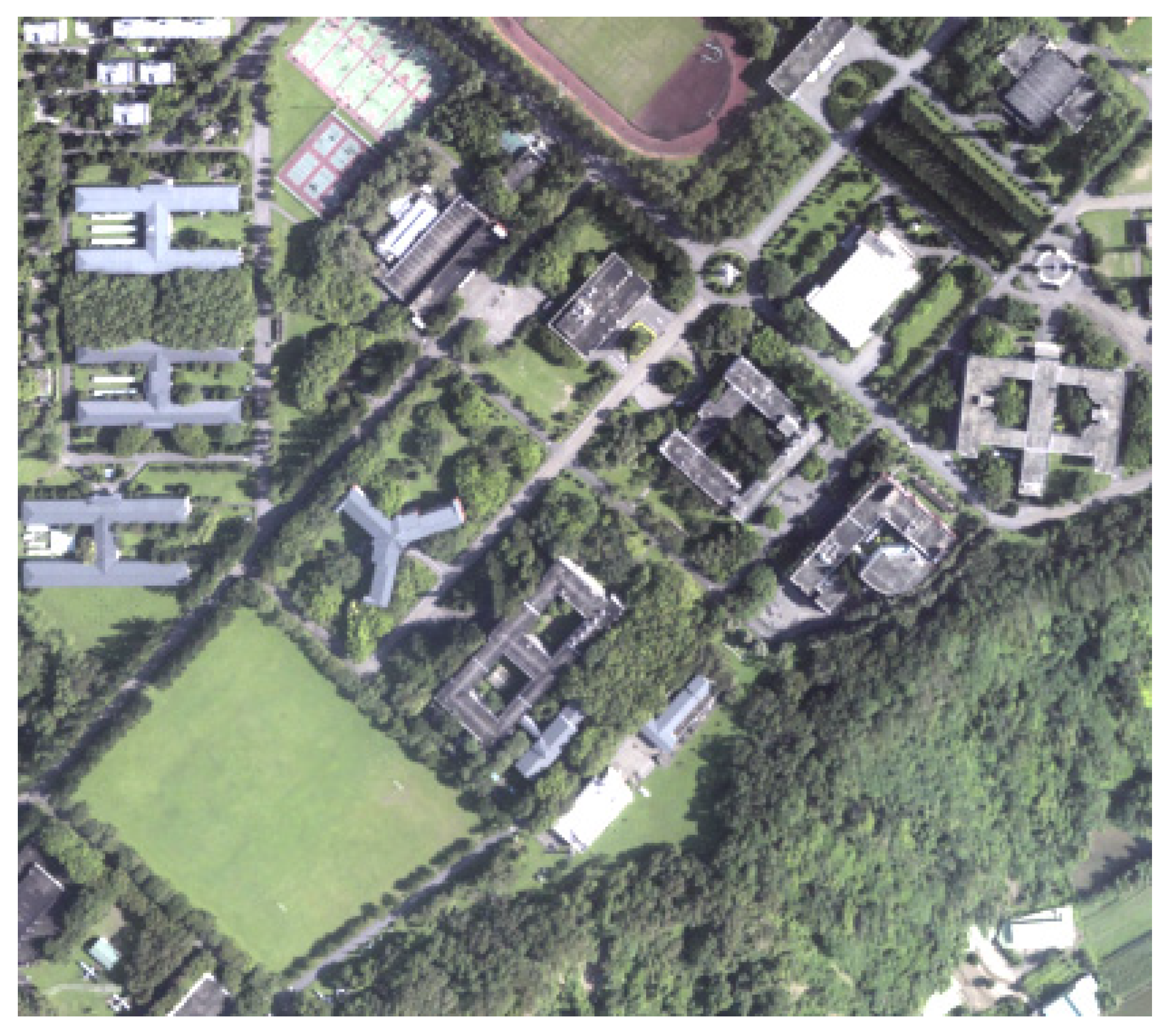
Figure 1.
Orthophoto of the study area. (650 m × 600 m).
Figure 1.
Orthophoto of the study area. (650 m × 600 m).
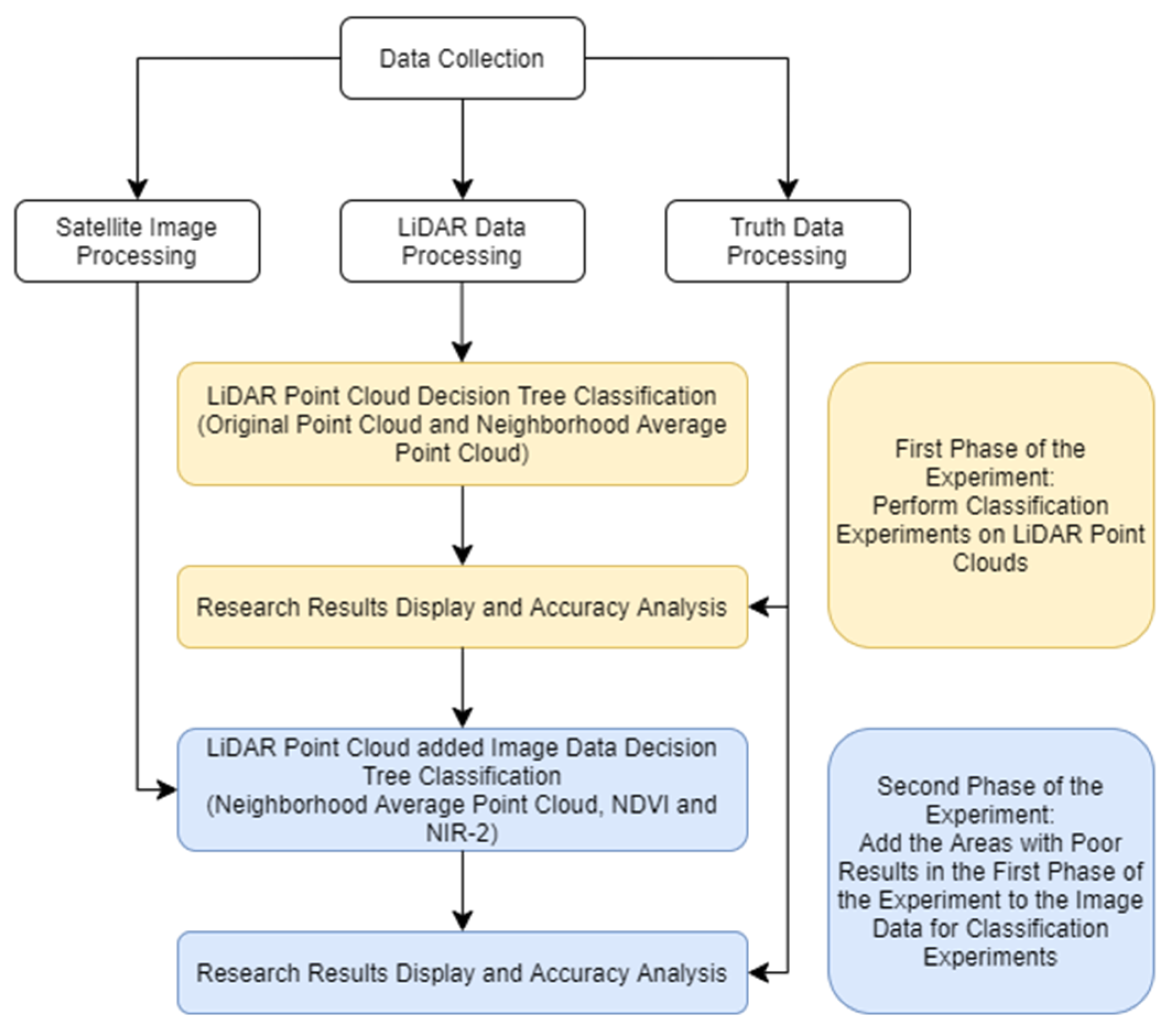
Figure 2.
Work Flow Chart.
Figure 2.
Work Flow Chart.
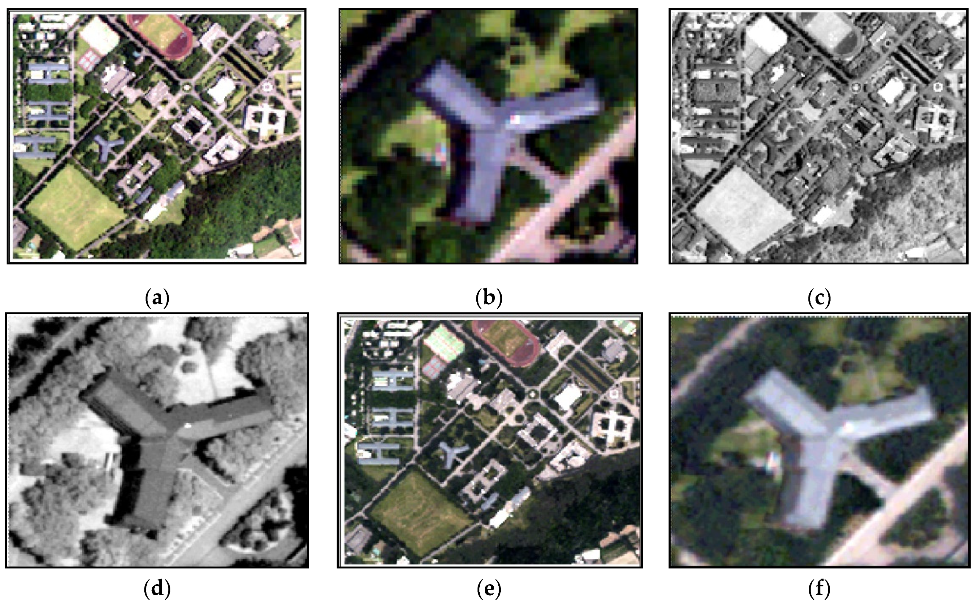
Figure 3.
Fusion processing. (a) Multispectral image; (b) Multispectral zoom image; (c) Full color image; (d) Full color zoom image; (e) Image after fusion; (f) Fusion zoom image.
Figure 3.
Fusion processing. (a) Multispectral image; (b) Multispectral zoom image; (c) Full color image; (d) Full color zoom image; (e) Image after fusion; (f) Fusion zoom image.
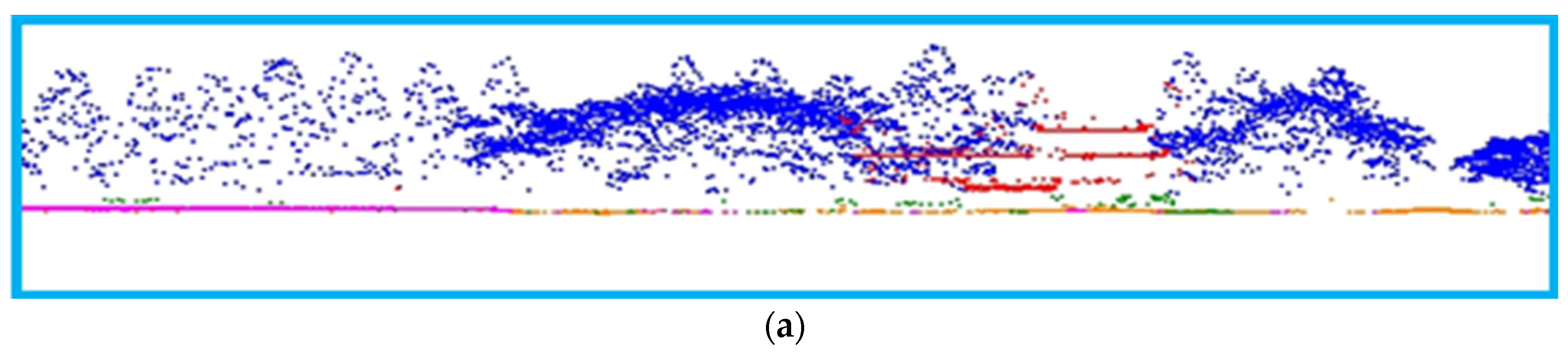
Figure 5.
Point cloud data of LiDAR’s two flight belts.
Figure 5.
Point cloud data of LiDAR’s two flight belts.
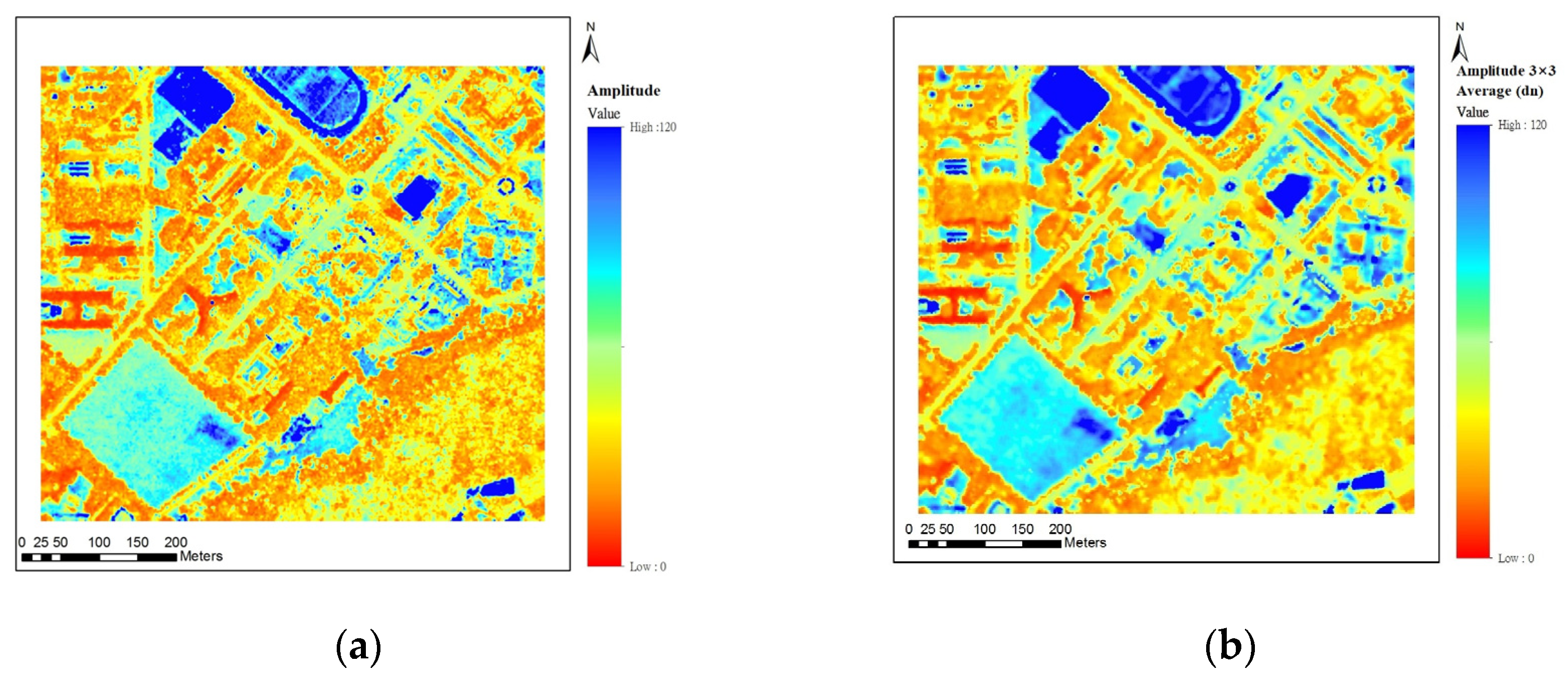
Figure 6.
Amplitude image. (a) Raw amplitude image; (b) Amplitude value image after neighborhood average.
Figure 6.
Amplitude image. (a) Raw amplitude image; (b) Amplitude value image after neighborhood average.
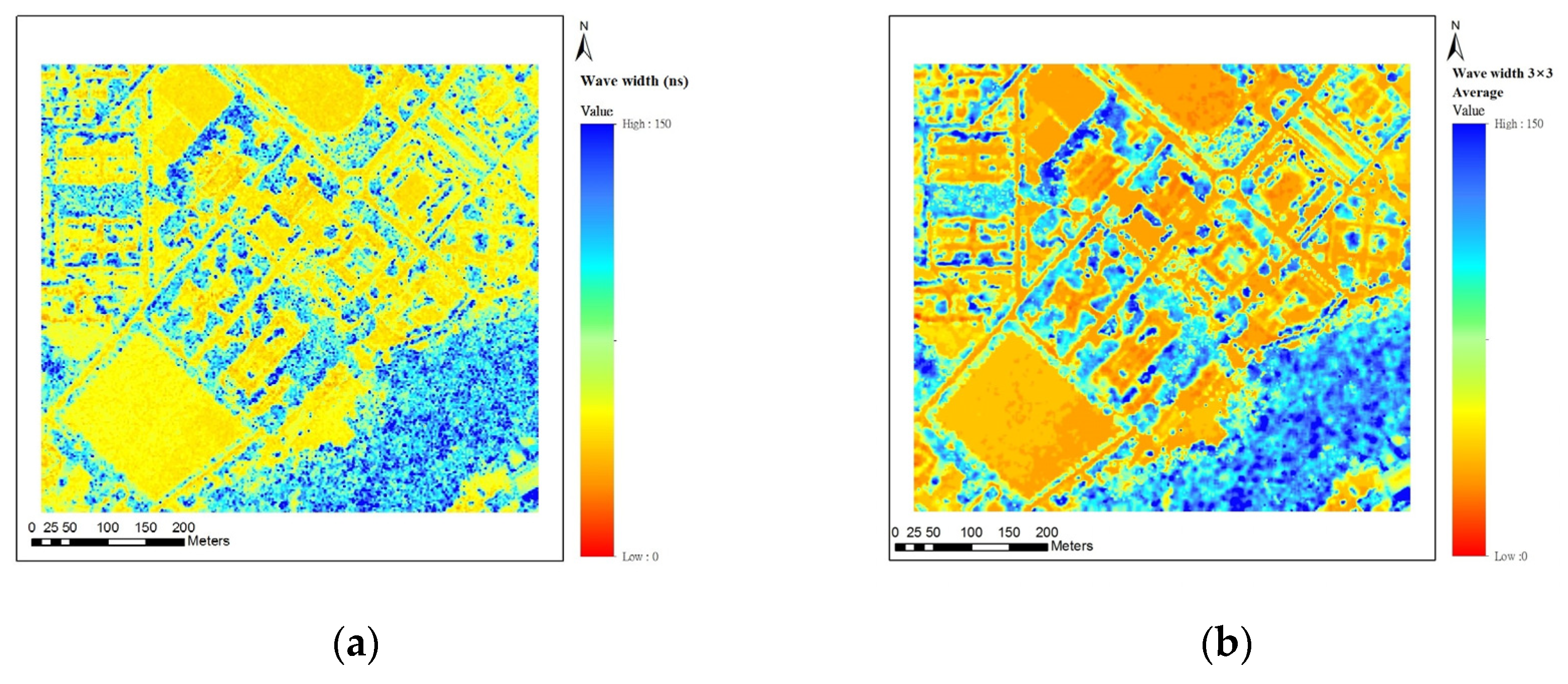
Figure 7.
Pulse width image. (a) Original pulse width image; (b) Pulse width value image after neighborhood average.
Figure 7.
Pulse width image. (a) Original pulse width image; (b) Pulse width value image after neighborhood average.
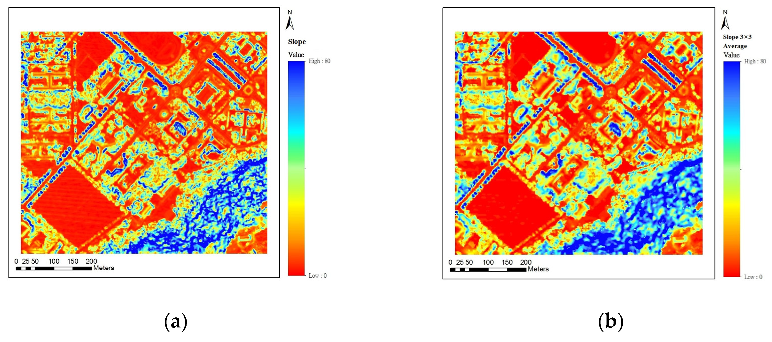
Figure 8.
Slope value image. (a) Original slope value image; (b) Slope value image after neighborhood average.
Figure 8.
Slope value image. (a) Original slope value image; (b) Slope value image after neighborhood average.
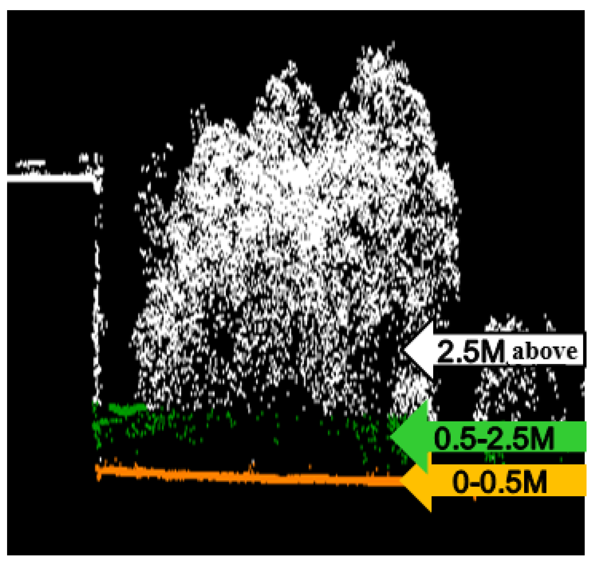
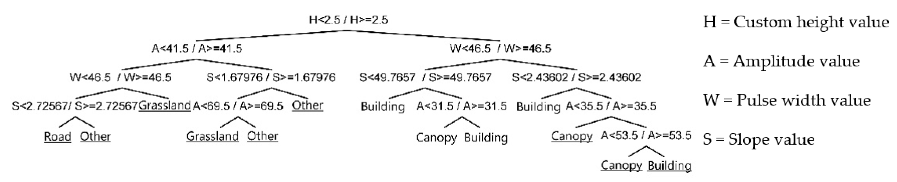
Figure 9.
Schematic diagram of custom height value.
Figure 9.
Schematic diagram of custom height value.
Figure 10.
Point cloud truth data.
Figure 10.
Point cloud truth data.
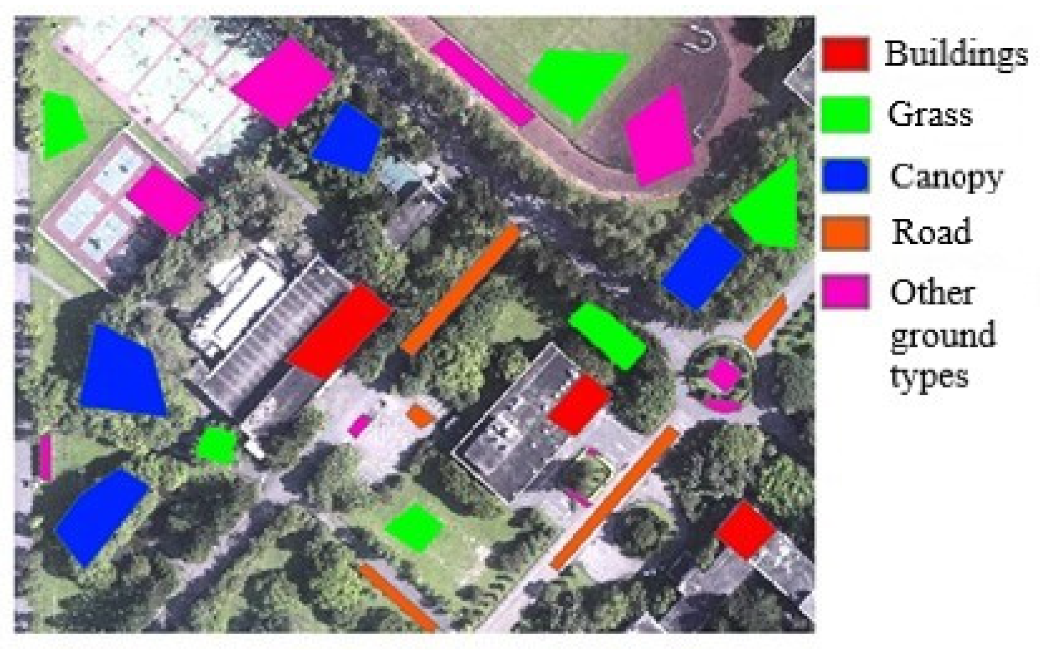
Figure 11.
Sampling diagram of training samples in the first phase of the experimental study area.
Figure 11.
Sampling diagram of training samples in the first phase of the experimental study area.
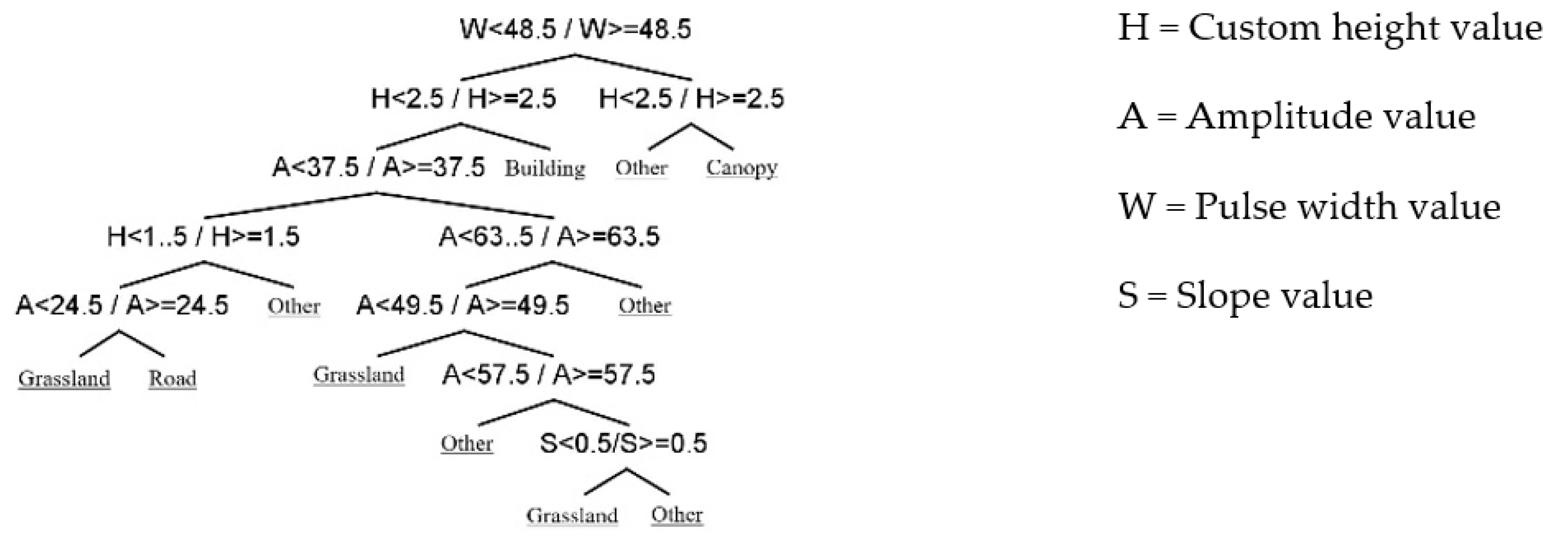
Figure 12.
Pruning the decision tree with the original value of the first stage experiment.
Figure 12.
Pruning the decision tree with the original value of the first stage experiment.
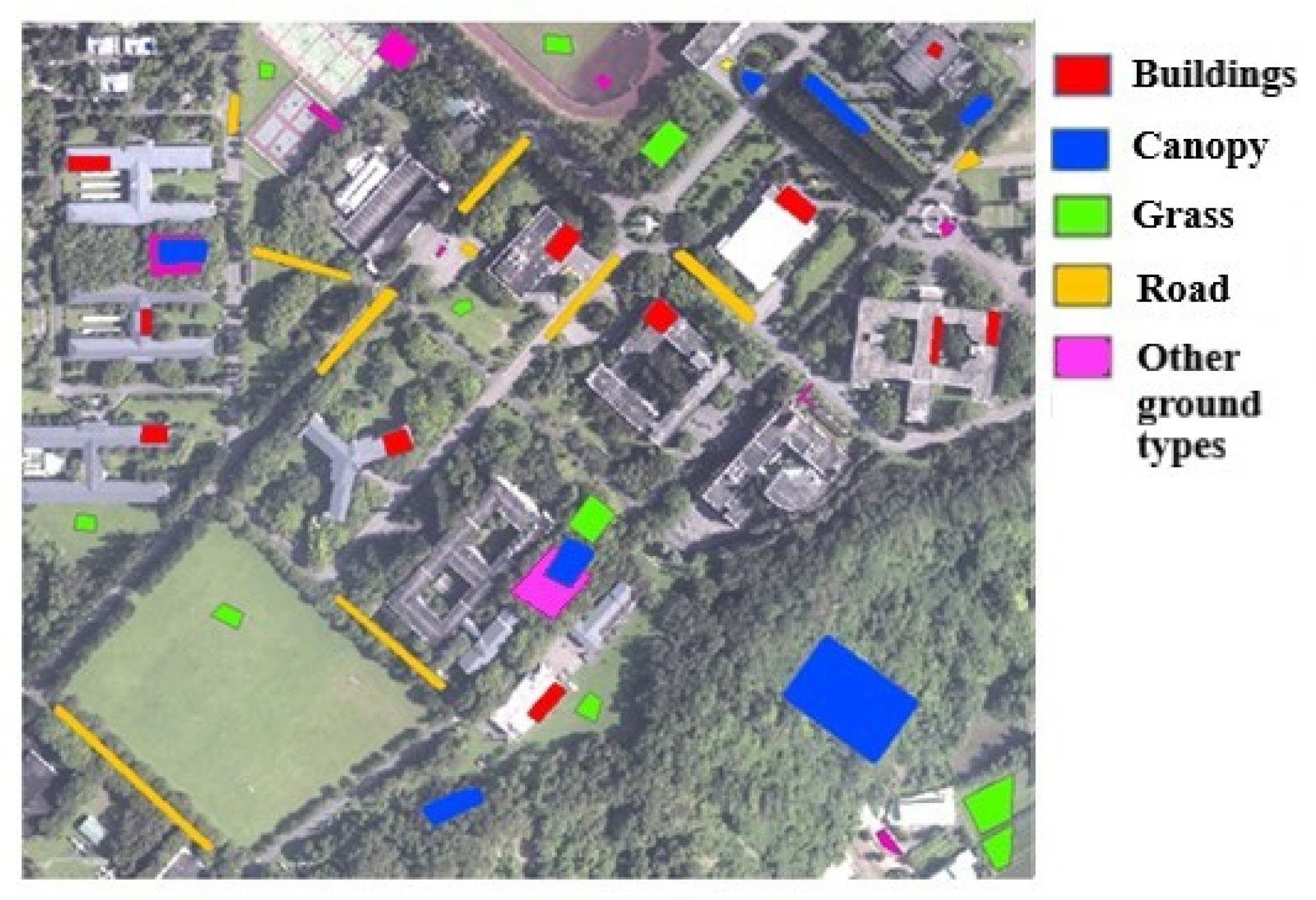
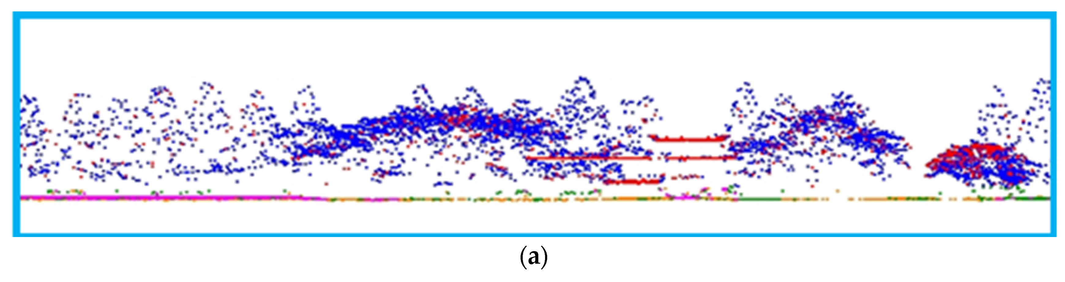
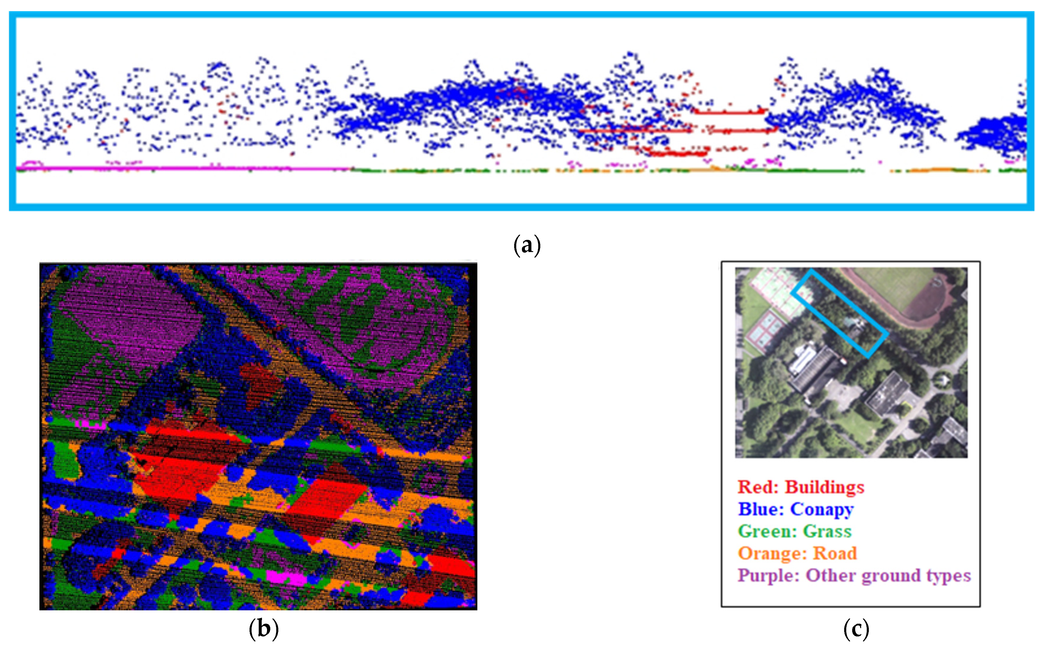
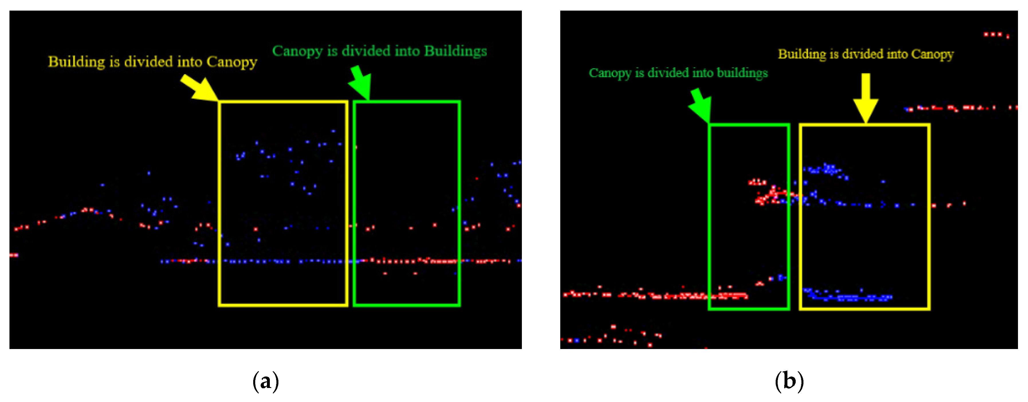
Figure 13.
Classification results of the original value of the first stage experiment. (a) Local point cloud profile results; (b) Point cloud classification results in the study area; (c) Comparison diagram.
Figure 13.
Classification results of the original value of the first stage experiment. (a) Local point cloud profile results; (b) Point cloud classification results in the study area; (c) Comparison diagram.
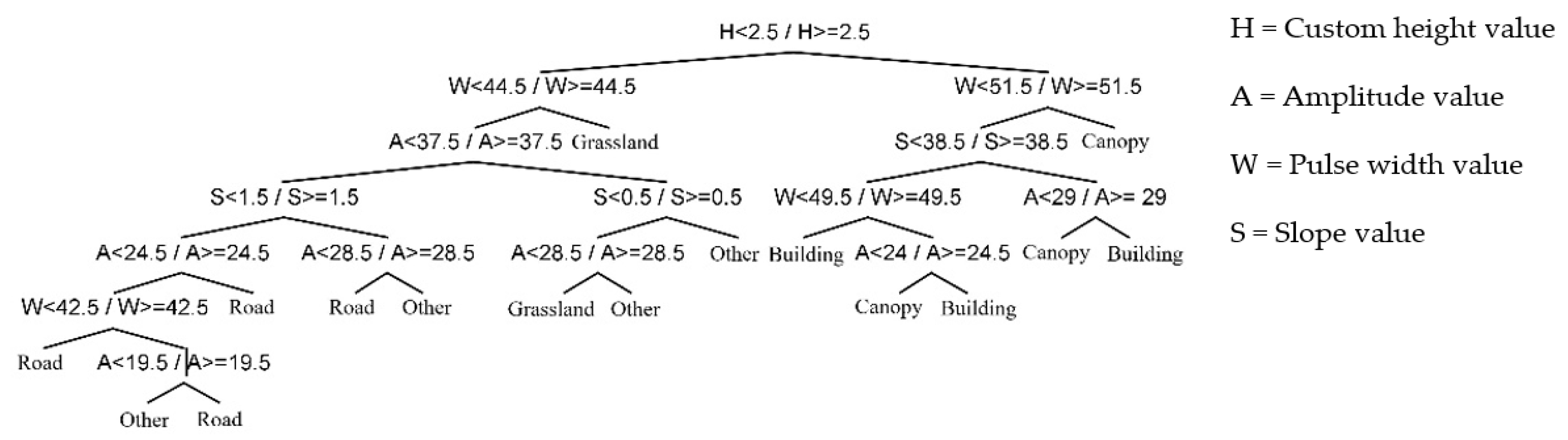
Figure 14.
Decision tree trimmed by the mean value of neighborhood in the first stage experiment.
Figure 14.
Decision tree trimmed by the mean value of neighborhood in the first stage experiment.
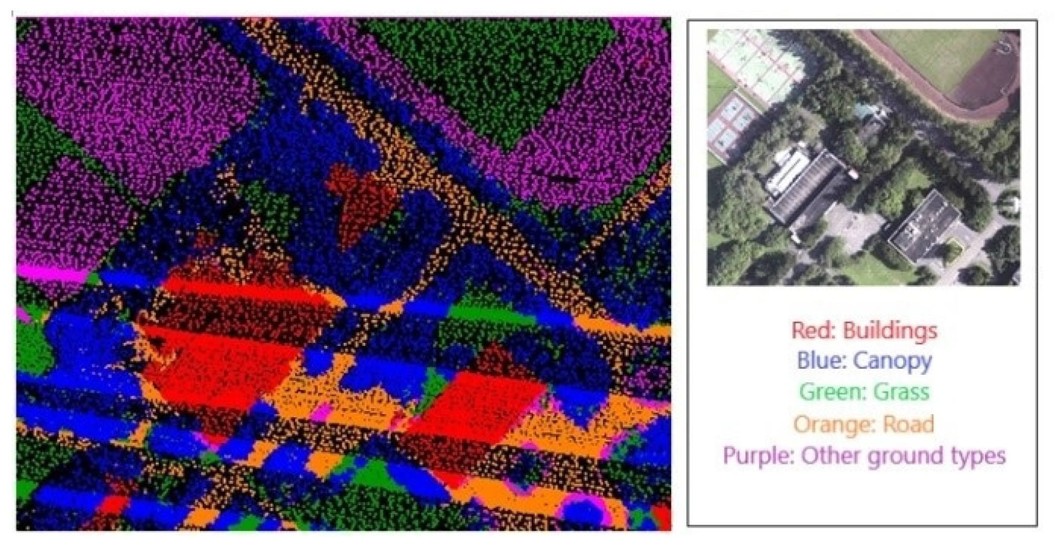
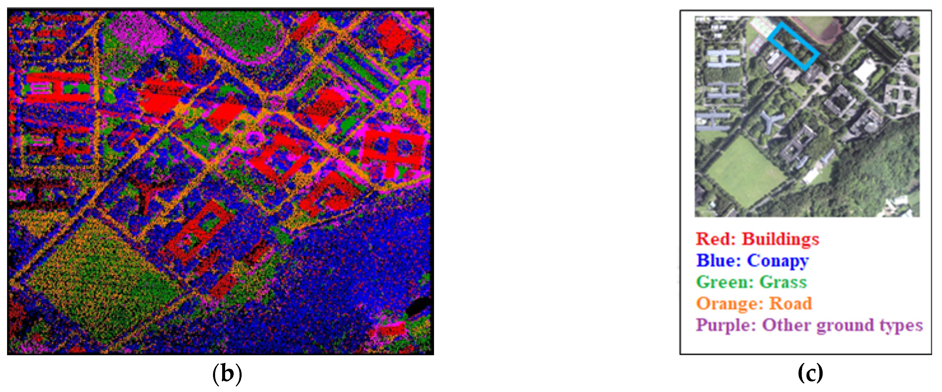
Figure 15.
Results of the neighborhood average classification in the first phase of the experiment. (a) Local point cloud profile results; (b) Point cloud classification results in the study area; (c) Comparison diagram.
Figure 15.
Results of the neighborhood average classification in the first phase of the experiment. (a) Local point cloud profile results; (b) Point cloud classification results in the study area; (c) Comparison diagram.
Figure 16.
Sampling diagram of training samples in the second phase experimental study area.
Figure 16.
Sampling diagram of training samples in the second phase experimental study area.
Figure 17.
Pruning the decision tree by the average value of the experimental neighborhood in the second stage.
Figure 17.
Pruning the decision tree by the average value of the experimental neighborhood in the second stage.
Figure 18.
Results of the neighborhood average classification in the second experiment. (a) Local point cloud profile results; (b) Point cloud classification results in the study area; (c) Comparison diagram.
Figure 18.
Results of the neighborhood average classification in the second experiment. (a) Local point cloud profile results; (b) Point cloud classification results in the study area; (c) Comparison diagram.
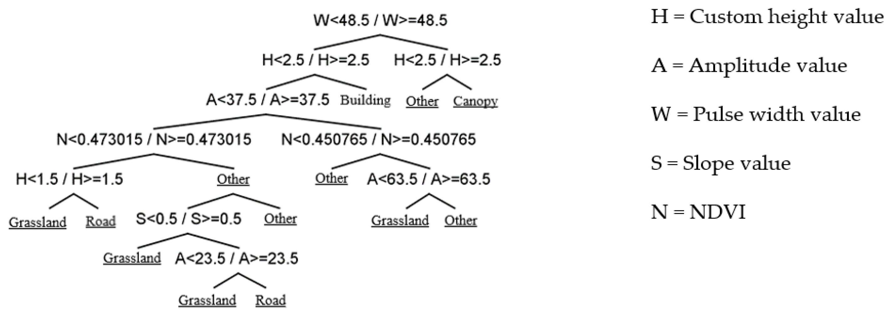
Figure 19.
The second stage experiment adds NDVI value to trim the decision tree.
Figure 19.
The second stage experiment adds NDVI value to trim the decision tree.
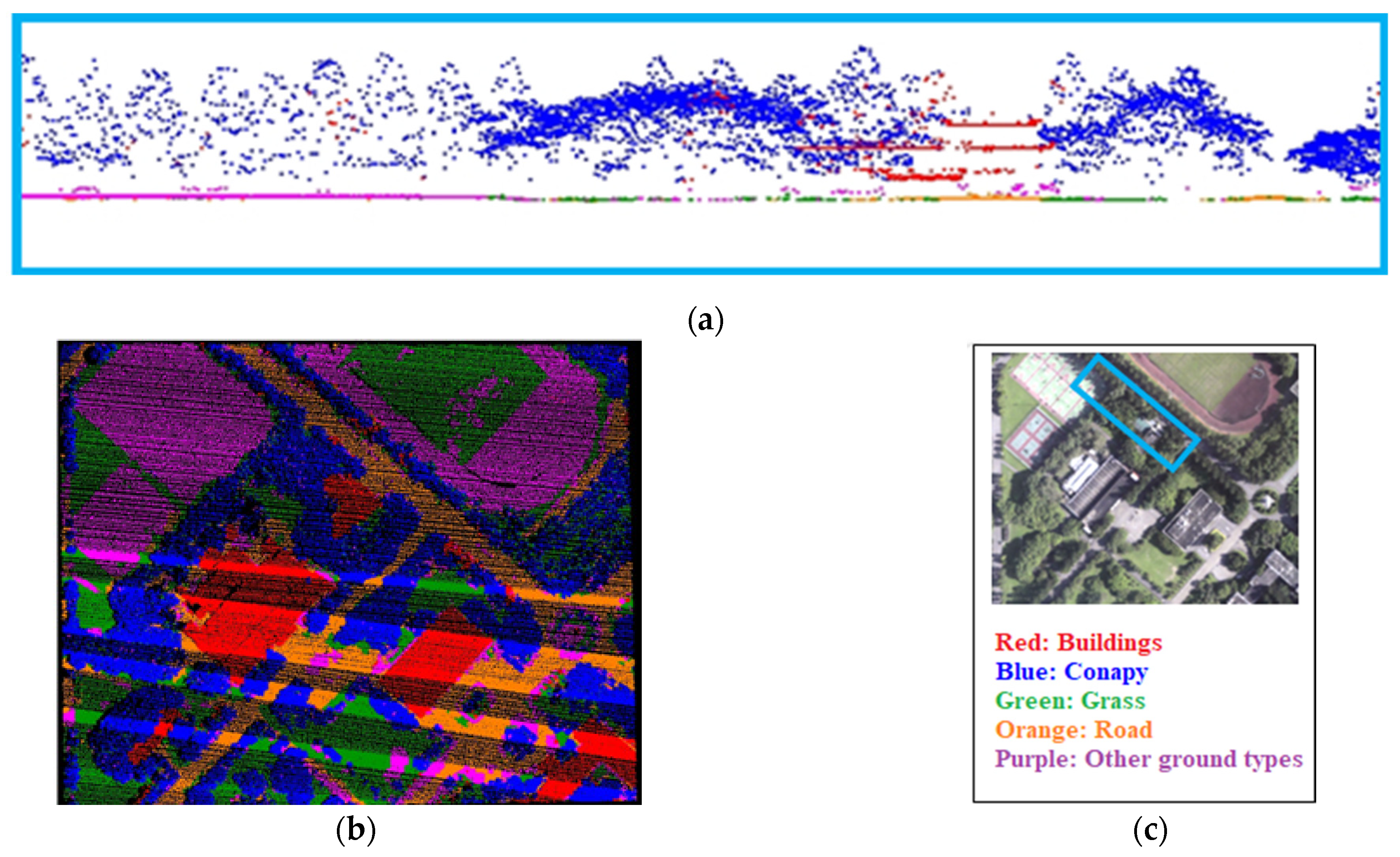
Figure 20.
The second stage experiment added NDVI value classification results. (a) Local point cloud profile results; (b) Point cloud classification results in the study area; (c) Comparison diagram.
Figure 20.
The second stage experiment added NDVI value classification results. (a) Local point cloud profile results; (b) Point cloud classification results in the study area; (c) Comparison diagram.
Figure 21.
The second stage experiment adds image NIR-2 value to trim the decision tree.
Figure 21.
The second stage experiment adds image NIR-2 value to trim the decision tree.
Figure 22.
The second stage experiment added image NIR-2 value classification results. (a) Local point cloud profile results; (b) Point cloud classification results in the study area; (c) Comparison diagram.
Figure 22.
The second stage experiment added image NIR-2 value classification results. (a) Local point cloud profile results; (b) Point cloud classification results in the study area; (c) Comparison diagram.
Figure 23.
(a) Neighborhood average limit graph I; (b) Neighborhood average limit graph II.
Figure 23.
(a) Neighborhood average limit graph I; (b) Neighborhood average limit graph II.
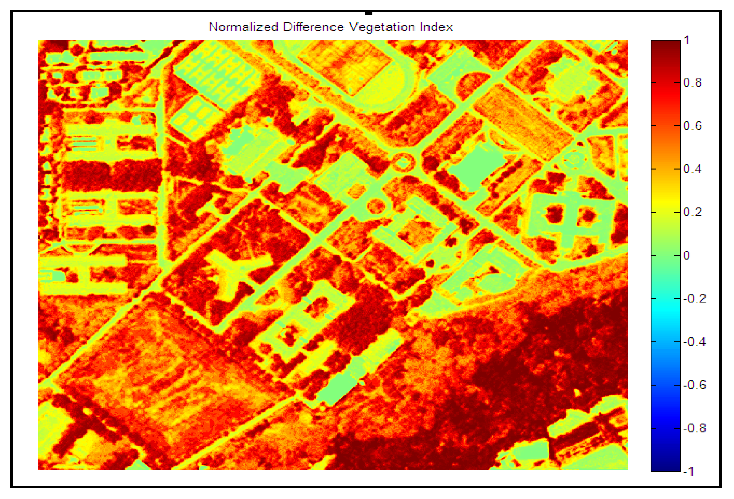
Figure 24.
Vegetation Difference Image. (a) Satellite imagery; (b) Aerial photograph.
Figure 24.
Vegetation Difference Image. (a) Satellite imagery; (b) Aerial photograph.
Table 1.
Error Matrix.
| Classification Results | Ground Truth |
|---|
| Class A | Class B | … | Class N | Total Category Pixels | PA |
|---|
| Class a | X(1, 1) | X(1, 2) | … | X(1, N) | | |
| Class b | X(2, 1) | X(2, 2) | … | X(2, N) | | |
| ⋮ | ⋮ | ⋮ | ⋮ | ⋮ | ⋮ | ⋮ |
| Class n | X(n, 1) | X(n, 2) | … | X(n, N) | | |
| Total Ground truth Category | | | … | | | |
| UA | | | … | | | |
Table 2.
Training Amplitude Value–Comparison Table of Original Value and Neighborhood Standard Deviation.
Table 2.
Training Amplitude Value–Comparison Table of Original Value and Neighborhood Standard Deviation.
| Amplitude Value (Unit: DN) |
|---|
| | Method | Original Mean | Original Value Standard Deviation | Neighborhood Average | Neighborhood Standard Deviation | The Average Standard Deviation of Various Neighborhoods Decreases |
|---|
| Category | |
|---|
| Buildings | 32.72 | 17.7 | 35.18 | 16.60 | 6.32% |
| Tree | 21.92 | 8.02 | 21.42 | 3.61 | 55.04% |
| Other ground | 2.49 | 3.41 | 1.72 | 2.37 | 30.40% |
| Grass | 32.67 | 13.69 | 32.30 | 11.50 | 16.00% |
| Road | 28.21 | 7.45 | 28.13 | 5.3 | 28.94% |
| Overall standard deviation | 50.27 | | 39.38 | |
| Neighborhood average overall standard deviation decreases: 21.61% |
Table 3.
Comparison table of training pulse width value–original value and neighborhood mean standard deviation.
Table 3.
Comparison table of training pulse width value–original value and neighborhood mean standard deviation.
| Amplitude Value (Unit: DN) |
|---|
| | Method | Original Mean | Original Value Standard Deviation | Neighborhood Average | Neighborhood Standard Deviation | The Average Standard Deviation of Various Neighborhoods Decreases |
|---|
| Category | |
|---|
| Buildings | 45.19 | 6.11 | 44.84 | 2.71 | 55.60% |
| Tree | 54.96 | 9.69 | 54.45 | 2.26 | 76.68% |
| Other ground | 43.64 | 2.46 | 43.17 | 1.15 | 53.21% |
| Grass | 47.21 | 7.46 | 46.82 | 5.74 | 23.04% |
| Road | 43.31 | 1.95 | 42.96 | 0.57 | 70.92% |
| Overall standard deviation | 27.68 | | 12.43 | |
| Neighborhood average overall standard deviation decreases: 55.07% |
Table 4.
Training slope value–original value and neighborhood standard deviation comparison table.
Table 4.
Training slope value–original value and neighborhood standard deviation comparison table.
| Amplitude Value (Unit: DN) |
|---|
| | Method | Original Mean | Original Value Standard Deviation | Neighborhood Average | Neighborhood Standard Deviation | The Average Standard Deviation of Various Neighborhoods Decreases |
|---|
| Category | |
|---|
| Buildings | 16.39 | 17.13 | 15.62 | 12.60 | 26.44% |
| Tree | 33.56 | 15.83 | 33.09 | 11.99 | 24.26% |
| Other ground | 2.49 | 3.41 | 1.723 | 2.37 | 30.40% |
| Grass | 1.22 | 1.45 | 0.74 | 1.19 | 18.16% |
| Road | 1.02 | 0.62 | 0.64 | 0.507 | 17.83% |
| Overall standard deviation | 38.43 | | 28.65 | |
| Neighborhood average overall standard deviation decreases: 25.45% |
Table 5.
Error matrix of original value in the first stage experiment.
Table 5.
Error matrix of original value in the first stage experiment.
| Classification Results | Buildings | Canopy | Road | Grassland | Other Ground | Classification Total | Producer Accuracy (PA) |
|---|
| Buildings | 22,153 | 6073 | 0 | 0 | 42 | 28,268 | 78% |
| Canopy | 2362 | 38,226 | 0 | 0 | 8 | 40,596 | 94% |
| Road | 0 | 34 | 26,471 | 7081 | 2044 | 35,630 | 74% |
| Grassland | 4 | 419 | 3679 | 10,129 | 7738 | 21,969 | 46% |
| Other ground | 2 | 63 | 2537 | 1659 | 7224 | 11,485 | 63% |
| Ground truth category total | 24,521 | 44,815 | 32,687 | 18,869 | 17,056 | 137,948 | |
| User Accuracy (UA) | 90% | 85% | 81% | 54% | 42% | | |
| Overall Accuracy (OA): 76%, Kappa: 43.26% |
Table 6.
The mean error matrix of the neighborhood in the first stage experiment.
Table 6.
The mean error matrix of the neighborhood in the first stage experiment.
| Classification Results | Buildings | Canopy | Road | Grassland | Other Ground | Classification Total | Producer Accuracy (PA) |
|---|
| Buildings | 23,648 | 988 | 0 | 0 | 31 | 24,667 | 96% |
| Canopy | 866 | 43,328 | 0 | 0 | 19 | 44,213 | 98% |
| Road | 0 | 18 | 28,377 | 4536 | 687 | 33,618 | 84% |
| Grassland | 7 | 477 | 1133 | 11,038 | 8070 | 20,725 | 53% |
| Other ground | 0 | 4 | 3177 | 3295 | 8249 | 14,725 | 56% |
| Ground truth category total | 24,521 | 44,815 | 32,687 | 18,869 | 17,056 | 137,948 | |
| User Accuracy (UA) | 96% | 97% | 87% | 58% | 48% | | |
| Overall Accuracy (OA): 83%, Kappa: 49.18% |
Table 7.
Neighbor mean error matrix of the second stage experiment.
Table 7.
Neighbor mean error matrix of the second stage experiment.
| Classification Results | Buildings | Canopy | Road | Grassland | Other Ground | Classification Total | Producer Accuracy (PA) |
|---|
| Buildings | 24,029 | 1355 | 0 | 0 | 31 | 25,415 | 95% |
| Canopy | 485 | 42,961 | 0 | 0 | 19 | 43,465 | 99% |
| Road | 0 | 12 | 28,395 | 2965 | 1055 | 32,427 | 88% |
| Grassland | 2 | 0 | 3985 | 13,464 | 4712 | 22,163 | 61% |
| Other ground | 5 | 487 | 339 | 2440 | 11,239 | 14,510 | 77% |
| Ground truth category total | 24,521 | 44,815 | 32,687 | 18,869 | 17,056 | 137,948 | |
| User Accuracy (UA) | 98% | 96% | 87% | 71% | 66% | | |
| Overall Accuracy (OA): 87%, Kappa: 52.60% |
Table 8.
Error matrix of neighborhood mean value plus NDVI value in the second stage experiment.
Table 8.
Error matrix of neighborhood mean value plus NDVI value in the second stage experiment.
| Classification Results | Buildings | Canopy | Road | Grassland | Other Ground | Classification Total | Producer Accuracy (PA) |
|---|
| Buildings | 24,029 | 1355 | 0 | 0 | 30 | 25,414 | 95% |
| Canopy | 485 | 42,961 | 0 | 0 | 19 | 43,465 | 99% |
| Road | 0 | 12 | 27,555 | 1001 | 591 | 29,159 | 94% |
| Grassland | 2 | 0 | 3185 | 16,345 | 651 | 20,183 | 81% |
| Other ground | 5 | 487 | 1947 | 1523 | 15,765 | 19,727 | 80% |
| Ground truth category total | 24,521 | 44,815 | 32,687 | 18,869 | 17,056 | 137,948 | |
| User Accuracy (UA) | 98% | 96% | 84% | 87% | 92% | | |
| Overall Accuracy (OA): 92%, Kappa: 56.85% |
Table 9.
Neighbor mean value plus NIR-2 value error matrix in the second stage experiment.
Table 9.
Neighbor mean value plus NIR-2 value error matrix in the second stage experiment.
| Classification Results | Buildings | Canopy | Road | Grassland | Other Ground | Classification Total | Producer Accuracy (PA) |
|---|
| Buildings | 24,029 | 1355 | 0 | 0 | 31 | 25,415 | 95% |
| Canopy | 485 | 42,961 | 0 | 0 | 19 | 43,465 | 99% |
| Road | 0 | 12 | 28,874 | 4200 | 1365 | 34,451 | 84% |
| Grassland | 2 | 0 | 2677 | 12,514 | 1725 | 16,918 | 74% |
| Other ground | 5 | 47 | 1136 | 2155 | 13,916 | 17,259 | 81% |
| Ground truth category total | 24,521 | 44,815 | 32,687 | 18,869 | 17,056 | 137,948 | |
| User Accuracy (UA) | 98% | 96% | 88% | 66% | 82% | | |
| Overall Accuracy (OA): 89%, Kappa: 53.81% |


