Targeting: Logistic Regression, Special Cases and Extensions

Abstract

Logistic regression is a classical linear model for logit-transformed conditional probabilities of a binary target variable. It recovers the true conditional probabilities if the joint distribution of predictors and the target is of log-linear form. Weights-of-evidence is an ordinary logistic regression with parameters equal to the differences of the weights of evidence if all predictor variables are discrete and conditionally independent given the target variable. The hypothesis of conditional independence can be tested in terms of log-linear models. If the assumption of conditional independence is violated, the application of weights-of-evidence does not only corrupt the predicted conditional probabilities, but also their rank transform. Logistic regression models, including the interaction terms, can account for the lack of conditional independence, appropriate interaction terms compensate exactly for violations of conditional independence. Multilayer artificial neural nets may be seen as nested regression-like models, with some sigmoidal activation function. Most often, the logistic function is used as the activation function. If the net topology, i.e., its control, is sufficiently versatile to mimic interaction terms, artificial neural nets are able to account for violations of conditional independence and yield very similar results. Weights-of-evidence cannot reasonably include interaction terms; subsequent modifications of the weights, as often suggested, cannot emulate the effect of interaction terms.

1. Introduction

The objective of potential modeling or targeting [1] is to identify locations, i.e., pixels or voxels, for which the probability of an event spatially referenced in this way, e.g., a well-defined type of ore mineralization, is relatively maximum, i.e., is larger than in neighbor pixels or voxels. The major prerequisite for such predictions is a sufficient understanding of the causes of the target to be predicted. Conceptual models of ore deposits have been compiled by [2]. They may be read as factor models (in the sense of mathematical statistics), and a proper factor model may be turned into a regression-type model when using the factors as spatially-referenced predictors, which are favorable to or prohibitive of the target event. Thus, we may distinguish necessary or sufficient dependencies between the binary target T(x) indicating the presence or absence of the target at an areal or volumetric location x ⊂ D ⊂ ℝ^d, d = 1, 2, 3, and the spatially referenced predictors (B₀(x), B₁(x),…, B_m(x))^T = B(x), which may be binary, discrete or continuous. Then, mathematical models and their numerical realizations are required to turn descriptive models into constructive ones, i.e., into quantitatively predictive models. Generally, a model considers the predictor B(x), with B₀(x) ≡ 1 for all x ⊂ D, and assigns a parameter (θ₀,…, θ_m)^T = θ to them, which quantifies, by means of a link function $ℱ$, the extent of dependence of the conditional probability P (T(x) = 1|B(x)) on the predictors, i.e.,

$$P(\mathrm{T}(x)=1|\mathbf{B}(x))=ℱ(\theta |\mathbf{B}(x))$$

Since the target T(x), as well as the predictor B(x) refer to areal or volumetric locations x ⊂ D, we may think of a two-dimensional digital map image of pixels or a three-dimensional digital geomodel of voxels. The pixels or voxels initially provide the physical support of the predictors and the target and will then be assigned the predicted conditional probability and the associated estimation errors, respectively. Then, the numerical results of targeting depend on the size of the objects, pixels or voxels, i.e., on the spatial resolution they provide. If the actual spatial reference of the target (or the predictors) is rather pointwise, i.e., if their physical support is rather of zero measure, then the dependence on the spatial resolution must not be ignored, because already, the estimate $\widehat{O}(\mathrm{T}=1)=\widehat{P}(\mathrm{T}=1)/(1-\widehat{P}(\mathrm{T}=1))$ of the unconditional odds will be largely affected, as the total number of pixels or voxels depends on the spatial resolution, while the total number of pointwise occurrences is constant. If the spatial resolution provided by the pixels or voxels is poor with respect to the area or volume of the actual physical support of the predictors or target, then the numerical results of any kind of mathematical method of targeting are rather an artifact of the inappropriate spatial resolution.

To estimate the model parameters θ, data within a training region are required. The mathematical modeling assumption associated with a training dataset is complete knowledge, i.e., in particular, we assume that we know all occurrences of the target variable T = 1. However, in contrast to geostatistics [3], potential modeling does not consider spatially-induced dependencies between the predictors and the target. In fact, potential modeling applies the assumption of independently identically distributed random variables. Their distribution does not depend on the location. Therefore, any spatial reference can be dropped, and models of the form:

$$P(\mathrm{T}=1|\mathbf{B})=ℱ(\theta |\mathbf{B})$$

are considered, only.

2. Mathematical Models

2.1. The Modeling Assumption of Conditional Independence

The random variables B₁,…, B_m are conditionally independent given the random target variable T, if the joint conditional probability factorizes into the individual conditional probabilities:

$$P_{{\otimes }_{\ell =1}^m{B}_{\ell }|\mathrm{T}}=\underset{\ell =1}{\overset{m}{{\displaystyle \otimes }}}{P}_{B_{\ell }|\mathrm{T}}$$

Equivalently, but more instructively in terms of irrelevance, the random variables B₁,…, B_m are conditionally independent given the random variable T, if knowing T renders all other B_j except B_i irrelevant for predicting B_i, i.e.,

$$P_{{\mathrm{B}}_i|{\otimes }_{\ell \ne i}{\mathrm{B}}_{\ell }\otimes \mathrm{T}}=P_{{\mathrm{B}}_i|\mathrm{T}}$$

in terms of conditional probabilities.

It is emphasized that independence does not imply conditional independence and vice versa. The significant correlation of predictor variables does not imply that they are not conditionally independent. On the contrary, variables B₁ and B₂ may be significantly correlated and conditionally independent given the variable T, in particular when T can be interpreted to represent a common cause for B₁ and B₂, cf. the illustrative example [4]. In this way, conditional independence is a probabilistic approach to causality, while correlation is not. To relax the restrictive assumption that all predictor variables are conditionally independent given the target variable, the assumption of conditional independence of subsets of predictor variables, referred to as the Bayesian belief network, provides intermediate models that are less restrictive, but more tractable than general models [5]. A suitable choice of subsets are the cliques of the graphical model [6] representing the variables and their conditional independence relationships leading to interaction terms in logistic regression models [7].

2.2. Logistic Regression

A modern account of logistic regression is given by [8]. The conditional expectation of an indicator random target variable T given a (m + 1)-variate random predictor variable is equal to its conditional probability, i.e., for B = (B₀, B₁,…, B_m)^T with B₀ ≡ 1

$$\mathrm{E}(\mathrm{T}|\mathbf{B})=P(\mathrm{T}=1|\mathbf{B})$$

Omitting the binomially distributed error term ([8]), as is done often, the ordinary logistic regression model without interaction terms for the conditional probability to be predicted can be written as [8]:

• in terms of a logit:

  $$\log \mathrm{it}P(\mathrm{T}=1|\mathbf{B})={\beta }^{\mathrm{T}}\mathbf{B}={\beta }_0+{\displaystyle \sum _{\ell }{\beta }_{\ell }{\mathrm{B}}_{\ell }}$$

• in terms of a probability:

  $$P(\mathrm{T}=1|\mathbf{B})=\mathrm{\Lambda }({\beta }^{\mathrm{T}}\mathbf{B})=\mathrm{\Lambda }\left({\beta }_0+{\displaystyle \sum _{\ell }{\beta }_{\ell }{\mathrm{B}}_{\ell }}\right)$$

  (1)

• with the logistic function:

  $$\mathrm{\Lambda }(z)=\frac{1}{1-\exp (-z)}$$

The ordinary logistic regression model is optimum, i.e., it agrees with the true conditional probability, if the predictor variables are discrete and conditionally independent given the target variable [7]. Here, the predictor variables are assumed to be discrete to ensure that the joint probability of B and T has a representation as a log-linear model, which is then subject to factorization, according to the Hammersley–Clifford theorem [7].

The logistic regression model can be generalized to include any interaction terms of the form $B_{{\ell }_i}*\dots *B_{{\ell }_j}$, i.e., any product terms of predictors:

$$P(\mathrm{T}=1|\mathbf{B})=\mathrm{\Lambda }({\beta }_0+{\displaystyle \sum _{\ell }{\beta }_{\ell }{\mathrm{B}}_{\ell }+{\displaystyle \sum _{{\ell }_i,\dots ,{\ell }_j}{\beta }_{{\ell }_i,\dots ,{\ell }_j}{\mathrm{B}}_{{\ell }_i}\otimes \dots \otimes B_{{\ell }_j}}})$$

Lacking conditional independence can be exactly compensated for by corresponding interaction terms included in the logistic regression model, and the resulting logistic regression model with interaction terms is optimum for continuous predictor variables if the joint distribution of the target variable and the predictor variables is of a log-linear form. A log-linear form is ensured if the predictor variables are discrete. Thus, for discrete predictor variables, the logistic regression model, including appropriate interaction terms, is optimum [7].

Given m ≥ 2 predictor variables ${\mathrm{B}}_{\ell }\cancel{\equiv }1$, ℓ = 1,…, m, there is a total of ${\displaystyle \sum {}_{\ell =2}^m}\left(\begin{array}{c}m\\ \ell \end{array}\right)=2^m-(m+1)$ possible interaction terms. To be a feasible model, the total number 2^m of all possible terms would have to be reasonably smaller than the sample size n. However, the interaction term ${\mathrm{B}}_{\ell }{}_{{}_1}\otimes \dots \otimes {\mathrm{B}}_{\ell }{}_{{}_k}$, k ≤ m, is actually required if ${\mathrm{B}}_{\ell }{}_{{}_1},\dots ,{\mathrm{B}}_{{\ell }_k}$ are not conditionally independent given T.

Logistic regression parameters can be interpreted with respect to logits analogously to the parameters of linear regression model, e.g., β_ℓ represents the increment of logitP(T = 1|B) if B_ℓℓis increased by one unit [8]. There are more involved interpretations to come, cf. Appendix B.

Given a sample b_ℓ,i, t_i, i = 1,…, n, ℓ = 1,…, m, the parameters of the logistic regression model are estimated with the maximum likelihood method numerically realized in Fisher’s scoring algorithm (a form of Newton–Raphson, a special case of an iteratively reweighted least squares algorithm) and encoded in any major statistical software package.

2.3. Weights-of-Evidence

The model of weights-of-evidence is the special case of a logistic regression model without interaction terms, if all predictor variables are binary and conditionally independent given the target variable [9]. It reads, e.g., in terms of the conditional probability to be predicted:

$$P(T=1|\mathbf{B})=\mathrm{\Lambda }({\beta }^{\mathrm{T}}\mathbf{B})\mathrm{\Lambda }\left({\beta }_0+{\displaystyle \sum _{\ell :B_{\ell }=1}{\beta }_{\ell }}\right)$$

(2)

where:

$$\begin{array}{ccc}{\beta }_0=\log \mathrm{it}P\left(T=1\right)+W^{(0)},& {\beta }_{\ell }=C_{\ell },& \ell =1,\dots ,m\end{array}$$

(3)

with contrasts C_ℓ defined as:

$$\begin{array}{cc}{C}_{\ell }=W_{\ell }^{(1)}-W_{\ell }^{(0)},& \ell =1,\dots ,m\end{array}$$

with weights-of-evidence:

$$\begin{array}{cc}{W}_{\ell }^{(1)}=\ln \frac{P\left({\mathrm{B}}_{\ell }=1|\mathrm{T}=1\right)}{P\left({\mathrm{B}}_{\ell }=1|\mathrm{T}=0\right)},& W_{\ell }^{(0)}=\ln \frac{P\left({\mathrm{B}}_{\ell }=0|\mathrm{T}=1\right)}{P\left({\mathrm{B}}_{\ell }=0|\mathrm{T}=0\right)}\end{array}$$

(4)

and with:

$$W^{(0)}={\displaystyle \sum _{\ell =1}^m{W}_{\ell }^{(0)}}$$

provided that:

$$\begin{array}{ccc}P\left({\mathrm{B}}_{\ell }=i|\mathrm{T}=j\right)\ne 0,& i,j=0,1,& \ell =1,\dots ,m\end{array}$$

(5)

Since the model of weights-of-evidence [10–14] is based on the naive Bayesian approach [5,14–17] assuming conditional independence of B given T, it can be derived in elementary terms from Bayes’ theorem for indicator random variables B₀, B₁, …, B_m:

$$\begin{array}{l}\mathrm{O}(\mathrm{T}=1|\mathbf{B})=\mathrm{O}(\mathrm{T}=1)\frac{{\displaystyle {\prod }_{\ell =1}^{m}P({\mathrm{B}}_{\ell }|{\mathrm{B}}_0,\dots ,{\mathrm{B}}_{\ell -1},\mathrm{T}=1)}}{{\displaystyle {\prod }_{\ell =1}^{m}P({\mathrm{B}}_{\ell }|{\mathrm{B}}_0,\dots ,{\mathrm{B}}_{\ell -1},\mathrm{T}=0)}}\\ =\mathrm{O}(\mathrm{T}=1){\displaystyle \prod _{\ell =1}^m{F}_{\ell }}\end{array}$$

with:

$$F_{\ell }=\frac{P({\mathrm{B}}_{\ell }|{\mathrm{B}}_0,\dots ,{\mathrm{B}}_{\ell -1},\mathrm{T}=1)}{P({\mathrm{B}}_{\ell }|{\mathrm{B}}_0,\dots ,{\mathrm{B}}_{\ell -1},\mathrm{T}=0)},\ell =1,\dots ,m$$

(6)

where the (conditional) odds O of an event are defined as the ratio of the (conditional) probabilities of an event and its complement. Now, the naive Bayes’ assumption of conditional independence of all predictor variables B given the target variable T leads to the most efficient simplification:

$$F_{\ell }=\frac{P({\mathrm{B}}_{\ell }|\mathrm{T}=1)}{P({\mathrm{B}}_{\ell }|\mathrm{T}=0)},\ell =1,\dots ,m$$

and, in turn, to weights-of-evidence in terms of odds:

$$\mathrm{O}(\mathrm{T}=1|\mathbf{B})=\mathrm{O}(\mathrm{T}=1){\displaystyle \prod _{\ell =1}^m\frac{P({\mathrm{B}}_{\ell }|\mathrm{T}=1)}{P({\mathrm{B}}_{\ell }|\mathrm{T}=0)}}$$

i.e., updating the unconditional “prior” odds O(T = 1) by successive multiplication with “Bayes factors” P (B_ℓ | T = 1)/P (B_ℓ | T = 0) to result in final conditional “posterior” odds O(T = 1 | B) [13]; see Appendix 1 for a complete derivation.

Due to the simplifying assumption of conditional independence and in contrast to general logistic regression, the ratios of conditional probabilities involved in the definition of the weights of evidence, Equation (4), can be estimated by mere counting. Moreover, weights-of-evidence can easily be generalized to discrete random variables, as a discrete variable with s different states can be split into (s − 1) different binary random variables to be used in regression models.

2.4. Testing Conditional Independence

A straightforward test of conditional independence employs the relationship of weights-of-evidence and log-linear models. If predictor variables are discrete and conditionally independent given the target variable, then by virtue of the Hammersley–Clifford theorem, a correspondingly factorized simple log-linear model without interaction terms is sufficiently large to represent the joint distribution [7,9]. Thus, if the likelihood ratio test of this null-hypothesis with respect to an appropriate log-linear model leads to its reasonable rejection, then the assumption of conditional independence can be rejected, too. This test does not rely on any assumption involving the normal distribution, as the omnibus tests [18,19] do.

These omnibus tests use deviations of a characteristic of a fitted model $F\left(\tilde{\theta }|b_i,t_i,i=1,\dots ,n\right)$ from properties of the mathematical model $ℱ$(θ | B) known from probability and mathematical statistics, to interfere on the validity of the modeling assumption of conditional independence. The omnibus tests take as characteristic the mean of conditional probabilities over all objects, i.e., pixels or voxels, in the training dataset of sample size n,

$$\frac{1}{n}{\displaystyle \sum _{i=1}^{n}P(\mathrm{T}=1|\mathbf{B}={\mathrm{b}}_i)=P(\mathrm{T}=1)}$$

(7)

Thus, for a proper (“true”) model, the mean of $\widehat{P}(\mathrm{T}=1|\mathbf{B}={\mathrm{b}}_i),$ i = 1,…, n, is (approximately) equal to $\widehat{P}(\mathrm{T}=1)$, estimated by the relative frequency of T = 1 in the training dataset. Deviations of the mean from $\widehat{P}(\mathrm{T}=1)$ would indicate that the model may not be true. For a weights-of-evidence model, deviations could be caused by a lack of conditional independence, while for a logistic regression model, $\frac{1}{n}{\displaystyle \sum {}_{i=1}^n}\widehat{P}(\mathrm{T}=1|\mathbf{B}={\mathrm{b}}_i)=\widehat{P}(\mathrm{T}=1)$ is always satisfied (up to numerical accuracy). Based on Equation (7), [19] developed the omnibus test, and [18] the new omnibus test.

A more sophisticated statistical test for real predictor variables was recently suggested by [20].

2.5. Weights-of-Evidence vs. Logistic Regression

The parameters of ordinary logistic regression are equal to the contrasts of the weights, if all predictor variables are indicators and conditionally independent given the target variable. Thus, weights-of-evidence is the special case of ordinary logistic regression if the predictors B are indicator variables and conditional independent given T. The other way round, logistic regression is the canonical generalization of weights-of-evidence [14,17]. Note that the weights-of-evidence model cannot be enlarged to include interaction terms.

Generally, i.e., without assuming conditional independence, the relationship of ordinary logistic regression parameters and the contrast of weights of evidence is clearly non-linear [21,22]; see Appendix 2 for an explicit derivation.

When $\widehat{P}(\mathrm{T}=1|\mathbf{B}={\mathrm{b}}_i)$, i = 1, …, n, are estimated by maximum likelihood applied to the ordinary logistic regression model, Equation (7) always holds, because it is part of the maximum likelihood systems of equations. Having recognized weights-of-evidence as a special case of logistic regression, when predictors are indicator variables and conditionally independent given the target variable, the above comparison may now be seen as checking the statistics of different models. Analogously, the estimated contrasts ${\widehat{C}}_{\ell }$ of weights of evidence may be compared with the estimated logistic regression coefficients ${\widehat{\beta }}_{\ell }$_. Then, any deviation between them is indicative of violations of the modeling assumption of conditional independence.

2.6. Weights-of-Evidence vs. the τ- or ν-Model

The modeling assumption with respect to the factors of Equation (6) of the τ-model [23–25] is:

$$F_{\ell }={\left(\frac{P({\mathrm{B}}_{\ell }|\mathrm{T}=1)}{P({\mathrm{B}}_{\ell }|\mathrm{T}=0)}\right)}^{{\tau }_{\ell }},\ell =1,\dots ,m$$

Then, modified weights are defined as:

$$\begin{array}{cccc}{\tilde{W}}_{\ell }^{(1)}={\tau }_{\ell }^{(1)}{W}_{\ell }^{(1)},& {\tilde{W}}_{\ell }^{(0)}={\tau }_{\ell }^{(0)}{W}_{\ell }^{(0)},& {\tilde{C}}_{\ell }={\tilde{W}}_{\ell }^{(1)}-{\tilde{W}}_{\ell }^{(0)},& \ell =1,\dots ,m\end{array}$$

and:

$$\begin{array}{l}\log \mathrm{it}P\left(\mathrm{T}=1|\mathbf{B}\right)=\log \mathrm{it}P\left(\mathrm{T}=1\right)+{\tilde{W}}^{(0)}+{\displaystyle \sum _{\ell =1}^m{\tilde{C}}_{\ell }{\mathrm{B}}_{\ell }}\\ P\left(\mathrm{T}=1|\mathbf{B}\right)=\mathrm{\Lambda }\left(\log \mathrm{it}P\left(\mathrm{T}=1\right)+{\tilde{W}}^{(0)}+{\displaystyle \sum _{\ell =1}^m{\tilde{C}}_{\ell }{\mathrm{B}}_{\ell }}\right)\end{array}$$

with ${\tilde{W}}^{(0)}={\displaystyle \sum {}_{\ell =1}^m}{\tau }_{\ell }^{(0)}{W}_{\ell }^{(0)}$.

The modeling assumption with respect to the factors of Equation (6) of the ν-model [26,27] is:

$$F_{\ell }={\nu }_{\ell }\left(\frac{P({\mathrm{B}}_{\ell }|\mathrm{T}=1)}{P({\mathrm{B}}_{\ell }|\mathrm{T}=0)}\right),\ell =1,\dots ,m$$

Then, modified weights are defined as:

$$\begin{array}{cccc}{\tilde{\tilde{W}}}_{\ell }^{(1)}=\ln {\nu }_{\ell }^{(1)}+W_{\ell }^{(1)},& {\tilde{\tilde{W}}}_{\ell }^{(0)}=\ln {\nu }_{\ell }^{(0)}+W_{\ell }^{(0)},& {\tilde{\tilde{C}}}_{\ell }={\tilde{\tilde{W}}}_{\ell }^{(1)}-{\tilde{\tilde{W}}}_{\ell }^{(0)},& \ell =1,\dots ,m\end{array}$$

and:

$$\begin{array}{l}\log \mathrm{it}P\left(\mathrm{T}=1|\mathbf{B}\right)=\log \mathrm{it}P\left(\mathrm{T}=1\right)+{\tilde{\tilde{W}}}^{(0)}+{\displaystyle \sum _{\ell =1}^m{\tilde{\tilde{C}}}_{\ell }{\mathrm{B}}_{\ell }}\\ P\left(\mathrm{T}=1|\mathbf{B}\right)=\mathrm{\Lambda }\left(\log \mathrm{it}P\left(\mathrm{T}=1\right)+{\tilde{\tilde{W}}}^{(0)}+{\displaystyle \sum _{\ell =1}^m{\tilde{\tilde{C}}}_{\ell }{\mathrm{B}}_{\ell }}\right)\end{array}$$

with ${\tilde{\tilde{W}}}^{(0)}={\displaystyle \sum {}_{\ell =1}^m}\left(\ln {\nu }_{\ell }^{(0)}+W_{\ell }^{(0)}\right)$.

A this point, we may conclude that there is no way to emulate the effect of interaction terms of logistic regression models by manipulating the weights of evidence or their contrasts.

2.7. Artificial Neural Nets

General regression models can be tackled by various approaches of statistical learning, including artificial neural nets [15]. With respect to artificial neural nets and statistical learning [5,15,16,28], the logistic regression model, Equation (1),

$${\pi }_1({\mathrm{b}}_i)=P(\mathrm{T}=1|\mathbf{B}={\mathrm{b}}_i))=\mathrm{\Lambda }\left({\beta }_0+{\displaystyle \sum _{\ell =1}^m{\beta }_{\ell }{b}_{\ell ,i}}\right),i=1,\dots ,n$$

is called a single-layer perceptron or single-layer feed-forward artificial neural net; minimization of the sum of squared residuals is referred to as training; gradient methods to solve for the model parameters are referred to as the linear perceptron training rule; the stepsize along the negative gradient is called the learning rate, etc. The notion of random variables, conditional independence, estimation and estimation error and the significance of model parameters does not seem to exist in the realm of artificial neural nets, not even under new labels. Nevertheless, artificial neural nets may be seen as providing a generalization to enlarge the logistic regression model by way of nesting logistic regression models with or without interaction terms. A minor additional generalization is to replace the logistic function Λ by other sigmoidal functions and to model the conditional probability of a categorical variable T (of more than two categories) given predictor variables B.

The basic multi-layer neural network model can be described as a sequence of functional transformations [15,29–31], often depicted as a graph:

• input: predictor variables B;

• first layer: linear combinations ${\mathrm{A}}_j^{(1)}$, j = 1, …, J, of the predictor variables B, referred to as input units or activations:

  $${\mathrm{A}}_j^{(1)}={\displaystyle \sum _{\ell =0}^m{\beta }_{j\ell }^{(1)}{\mathrm{B}}_{\ell },j=1,\dots ,J}$$

  (8)
  or:
  $${\mathrm{A}}_j^{(1)}={\displaystyle \sum _{\ell =0}^m{\beta }_{j\ell }^{(1)}{\mathrm{B}}_{\ell }+{\displaystyle \sum _{{\ell }_i,\dots ,{\ell }_{i^{\prime }}}{\beta }_{j({\ell }_i,\dots ,{\ell }_{i^{\prime }})}^{(1)}{\mathrm{B}}_{{\ell }_i}\otimes \dots }\otimes {\mathrm{B}}_{{\ell }_i},j=1,\dots ,J}$$

  (9)
  to mimic interaction terms:

• hidden layer: each of them is subject to a transformation applying a nonlinear differentiable activation function h usually of sigmoidal shape, referred to as hidden units:

  $$Z_j=h\left({\mathrm{A}}_j^{(1)}\right),j=1,\dots ,J$$

• second layer: linear combinations ${\mathrm{A}}_j^{(2)}$, k = 1, …, K of hidden units, referred to as output unit activations:

  $${\mathrm{A}}_k^{(2)}={\displaystyle \sum _{j=0}^J{\beta }_{kj}^{(2)}{\mathrm{Z}}_j,k=1,\dots ,K}$$

• output: each of the output unit activations is subject to an activation function S, e.g., logistic function:

  $${\pi }_k=S\left(A_k^{(2)}\right),k=1,\dots ,K$$
  Then:
  $${\pi }_k(\mathbf{B})=P(\mathrm{T}=t_k|\mathbf{B}))=S\left({\displaystyle \sum _{j=0}^J{\beta }_{kj}^{(2)}h\underset{\text{hidden layer}}{\underbrace{\left({\displaystyle \sum _{\ell =0}^m{\beta }_{j\ell }^{(1)}{\mathrm{B}}_{\ell }}\right)}}}\right),k=1,\dots ,K$$

  (10)

If K = 1 and S = Λ, h = id, J = 0, then we are of course back to ordinary logistic regression, Equation (1). On the other hand, in Equation (10), the linear combination of predictors, as given by Equation (8), can easily be replaced by the enlarged combination, including interaction terms, as given by Equation (9), where the consideration of interactions terms requires a more versatile net topology. The lack of the notion of significant parameters and, in turn, significant models is prohibitive of the successive construction of proper models. Instead, all variables and a sufficiently versatile net topology are plugged in, and coefficients for all variables are determined numerically with some gradient method. This procedure does not seem to meet the idea of parsimonious models.

2.8. Balancing

Methods of statistical learning are prone to fail if the odds O(T = 1) are too small, cf. [32–37]. Simple balancing mimics preferential sampling, i.e., a new balanced dataset is constructed by weighting all objects with T = 1 with a weight 1 < μ ∈ ℝ. This kind of balancing immediately results in:

$$\mathrm{O}\left({\mathrm{T}}^{\mathrm{bal}}=1\right)=\mu \mathrm{O}\left(\mathrm{T}=1\right),\mathrm{O}\left({\mathrm{T}}^{\mathrm{bal}}=1|{\mathbf{B}}^{\mathrm{bal}}\right)=\mu \mathrm{O}\left(\mathrm{T}=1|\mathbf{B}\right)$$

and then in:

$$\begin{array}{c}\mathrm{logit}P\left({\mathrm{T}}^{\mathrm{bal}}=1\right)=\ln \mu +\mathrm{logit}P\left(\mathrm{T}=1\right)\\ \mathrm{logit}P\left({\mathrm{T}}^{\mathrm{bal}}=1|{\mathbf{B}}^{\mathrm{bal}}\right)=\ln \mu +\mathrm{logit}P\left(\mathrm{T}=1|\mathbf{B}\right)\end{array}$$

Moreover, if:

$$\log \mathrm{it}P\left({\mathrm{T}}^{\mathrm{bal}}=1|{\mathbf{B}}^{\mathrm{bal}}\right)=F\left(\theta |{\mathbf{B}}^{\mathrm{bal}}\right)$$

is a proper (“true”) model for the balanced sample, then:

$$ℱ\left(\theta |\mathbf{B}\right)=ℱ\left(\theta |{\mathbf{B}}^{\mathrm{bal}}\right)-\ln \mu$$

(11)

is a proper model of logitP (T = 1| B) with respect to the initial sample, and:

$$ℱ\left(\widehat{\theta }|\mathbf{B}\right)=ℱ\left(\widehat{\theta }|{\mathbf{B}}^{\mathrm{bal}}\right)-\ln \mu$$

whatever the proper models are. For instance, if ordinary logistic regression without interaction terms, i.e., assuming conditional independence,

$$\log \mathrm{it}P\left({\mathrm{T}}^{\mathrm{bal}}=1|{\mathbf{B}}^{\mathrm{bal}}\right)=\log \mathrm{it}P\left({\mathrm{T}}^{\mathrm{bal}}=1\right)+W^{(0)}+{\displaystyle \sum _{\ell =1}^m{\beta }_{\ell }{\mathrm{B}}_{\ell }}$$

is a proper model for the balanced sample, then:

$$\begin{array}{l}\log \mathrm{it}P(\mathrm{T}=1|\mathbf{B})={\beta }_0+{\displaystyle \sum _{\ell =1}^m{\beta }_{\ell }{\mathrm{B}}_{\ell }}\\ =\log \mathrm{it}P({\mathrm{T}}^{\mathrm{bal}}=1)=\ln \mu +W^{(0)}+{\displaystyle \sum _{\ell =1}^m{\beta }_{\ell }{\mathrm{B}}_{\ell }}\\ =\log \mathrm{it}P(\mathrm{T}=1)+W^{(0)}+{\displaystyle \sum _{\ell =1}^m{\beta }_{\ell }{\mathrm{B}}_{\ell }}\end{array}$$

is a proper model for the initial sample. Thus, balancing by weighting objects, pixels or voxels, supporting T = 1 with μ > 1, does exactly what it is designed for: it increases the odds O(T = 1) by a factor of μ and preserves proper models, i.e., their parameters, otherwise.

It is emphasized that Equation (11) holds for mathematical models, if they are proper. Then, Equation (11) may be read as back transformation of balancing by weighting objects with T = 1 with weight μ. It may not hold for fitted models, i.e., estimation of the parameters of a poor model may corrupt the equation; then, $ℱ\left(\widehat{\theta }|\mathbf{B}\right)\ne ℱ\left(\widehat{\theta }|{\mathbf{B}}^{\mathrm{bal}}\right)-\ln \mu$. Note that the weights of evidence are not all affected by this kind of balancing.

2.9. Numerical Complexity of Logistic Regression

Potential modeling with logistic regression using a 3D training dataset of n voxels and (m + 1) predictor variables to fit the regression parameters requires to resolve a system of (m + 1) non-linear equations. Usually, the total number of predictor variables is much smaller than the total number of voxels. Statisticians’ numerical method of choice is iteratively reweighted least squares. The numerical complexity of one iteration step is of the order of 2n(m + 1)² flops; the total number of iterations cannot generally be estimated. Considering the size of the problem for 3D geomodels with a reasonable spatial resolution clearly indicates that its numerical solution requires a highly efficient data management of 3D geomodels in voxel mode and very fast numerics based on massively parallel processing.

3. Examples

Both datasets are fabricated to serve certain purposes. The mathematical assumption associated with a training dataset is complete knowledge, i.e., in particular, we assume that we know all occurrences of the target variable T = 1. Otherwise, not even the odds or logits of T = 1 could be estimated properly. Thus, previously unknown occurrences or their probabilities cannot be predicted with respect to the training dataset. Comparing the estimated conditional probabilities with counted conditional frequencies provides a check of the appropriateness of the applied model. A more powerful check is to use only part of the data out of the training dataset to estimate the parameters of a model and, then, to validate the model with the remaining data that were not used before. All computations were done with the free statistical software, R [38].

3.1. Dataset RANKIT Revisited

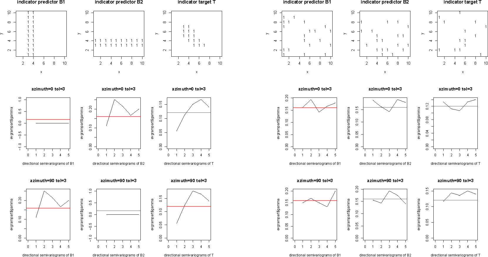
A first presentation and discussion of the dataset rankit (Figure 1) has been given in [9]. The rankit dataset comprises two predictor variables B₁, B₂ and a target variable T referring to pixels of a digital map image. The predictor variables B₁, B₂ are uncorrelated and not conditionally independent given the target variable T.

Here, the example is completed by considering a randomly rearranged dataset rankitmix (Figure 1), which originates from the dataset rankit by rearranging the pixel references (i, j) of triplets (b_k1, b_k2, t_k), k = 1, …, n, of realizations of B₁, B₂ and T in the dataset at random. The uni-directional variograms of Figure 1 clearly indicate that the two datasets differ in their spatial statistics.

However, the datasets rankit and rankitmix have identical ordinary statistics like contingency tables,

Table 1. Unconditional contingency table of B1 and B2, and conditional contingency tables of B₁ and B₂ given T of datasets rankit and rankitmix, respectively.

	B2 = 0	B2 = 1
B1 = 0	64	16
B1 = 1	16	4

T = 0	B2 = 0	B2 = 1
B1 = 0	62	11
B1 = 1	10	3

T = 1	B2 = 0	B2 = 1
B1 = 0	2	5
B1 = 1	6	1

and

Table 2. Contingency tables of T and B₁ and B₂, respectively, of datasets rankit and rankitmix, respectively.

	B2 = 0	B2 = 1
T = 0	73	13
T = 1	7	7

	B2 = 0	B2 = 1
T = 0	72	14
T = 1	8	6

, or a correlation matrix,

Table 3. Correlation matrix of the datasets rankit and rankitmix, respectively.

	B1	B2	T
B1	1.0000000	−0.0000000	0.3026050
B2	−0.0000000	1.0000000	0.2305562
T	0.3026050	0.2305562	1.0000000

, in common.

The indicator predictor variables B₁ and B₂ seem to be uncorrelated, while B₁ and T, and B₂ and T, respectively, are significantly correlated for all significance levels α > 0.002213 and α > 0.02101, respectively; cf. Table 3.

Therefore, for both the rankit and the rankitmix dataset, respectively, the models of weights-of-evidence, ordinary logistic regression without interaction term and enlarged logistic regression with the interaction term read explicitly:

$$\begin{array}{cc}\hfill \mathrm{WofE}:& \widehat{P}(\mathrm{T}=1|{\mathrm{B}}_1{\mathrm{B}}_2)=\mathrm{\Lambda }\left(-2.726+1.725{\mathrm{B}}_1+1.349{\mathrm{B}}_2\right)\hfill \\ \hfill \mathrm{ologReg}:& \widehat{P}(\mathrm{T}=1|{\mathrm{B}}_1{\mathrm{B}}_2)=\mathrm{\Lambda }\left(-2.831+1.874{\mathrm{B}}_1+1.535{\mathrm{B}}_2\right)\hfill \\ \hfill \mathrm{logRegwI}:& \widehat{P}(\mathrm{T}=1|{\mathrm{B}}_1{\mathrm{B}}_2)=\mathrm{\Lambda }\left(-3.434+2.923{\mathrm{B}}_1+2.646{\mathrm{B}}_2-3.233{\mathrm{B}}_1{\mathrm{B}}_2\right)\hfill \end{array}$$

Since the mathematical modeling assumption of conditional independence is violated, only logistic regression with interaction terms yields a proper model and predicts the conditional probabilities almost exactly.

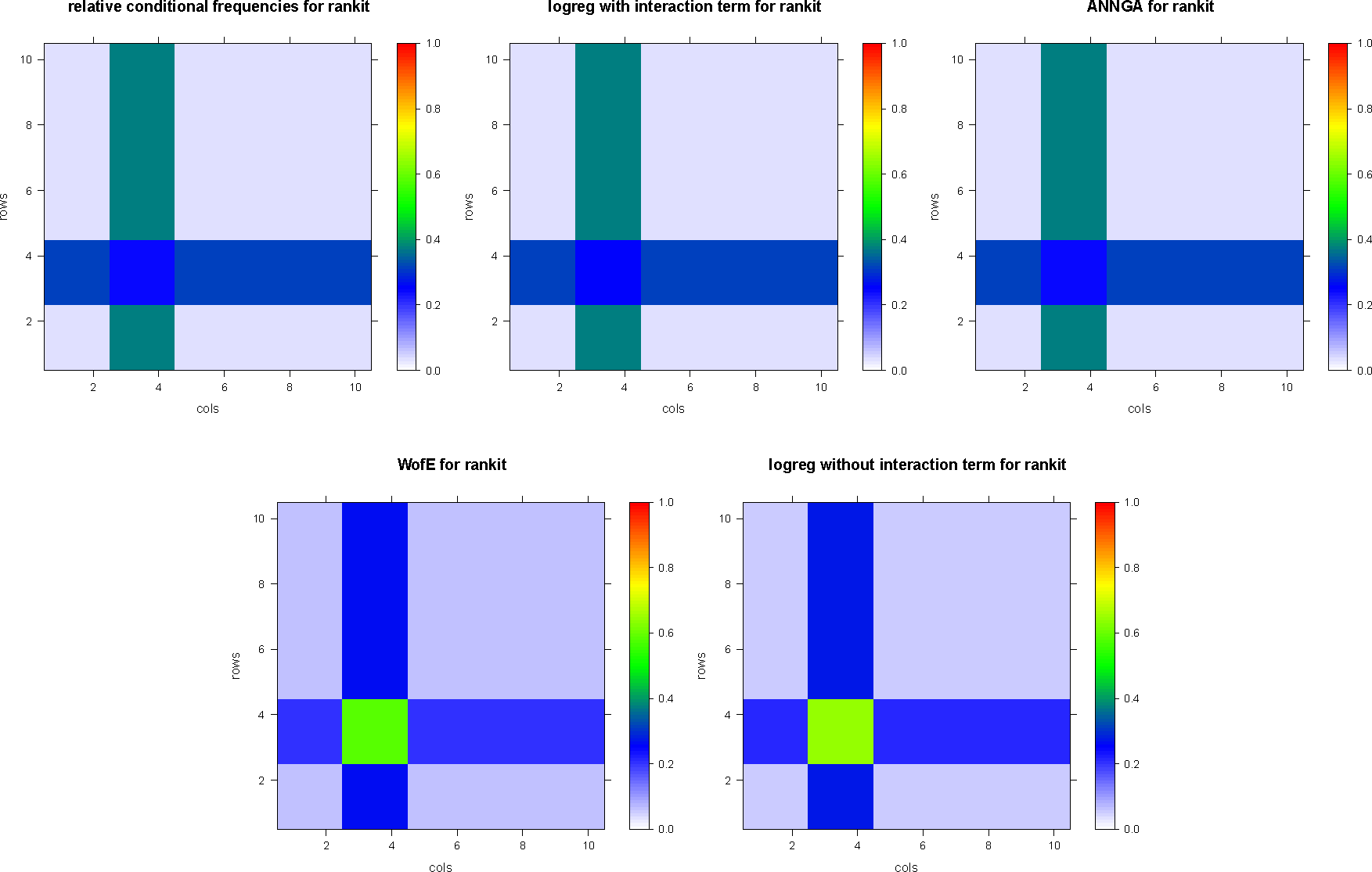
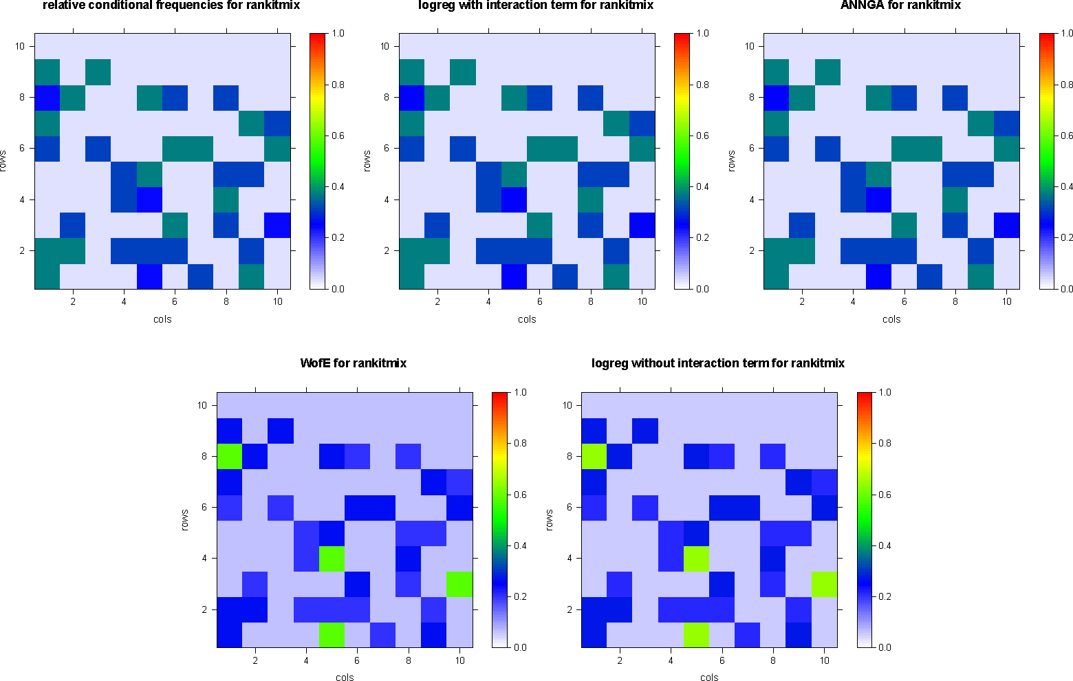
The results of weights-of-evidence, logistic regression with or without interaction terms and artificial neural net applied to the fabricated datasets rankit and the rankitmix dataset, respectively, are summarized in

Table 4. Comparison of conditional probabilities predicted with elementary counting, weights-of-evidence (WofE), ordinary logistic regression without interaction terms (oLogReg), logistic regression including interaction terms (LogRegwI), and artificial neural nets using a genetic algorithm (ANNGA [38]) applied to the training dataset rankit.

$\widehat{P}\left(\mathrm{T}=1|{\mathrm{B}}_1{\mathrm{B}}_2\right)$	Counting	WofE	oLogReg	LogRegwI	ANNGA
B1 = 1, B2 = 1	0.25000	0.58636	0.64055	0.25000	0.24992
B1 = 1, B2 = 0	0.37500	0.26875	0.27736	0.37500	0.37502
B1 = 0, B2 = 1	0.31250	0.20156	0.21486	0.31250	0.31250
B1 = 0, B2 = 0	0.03125	0.06142	0.05565	0.03125	0.03124

. Figure 2 depicts the results of dataset rankit, and Figure 3 depicts the results of dataset rankitmix.

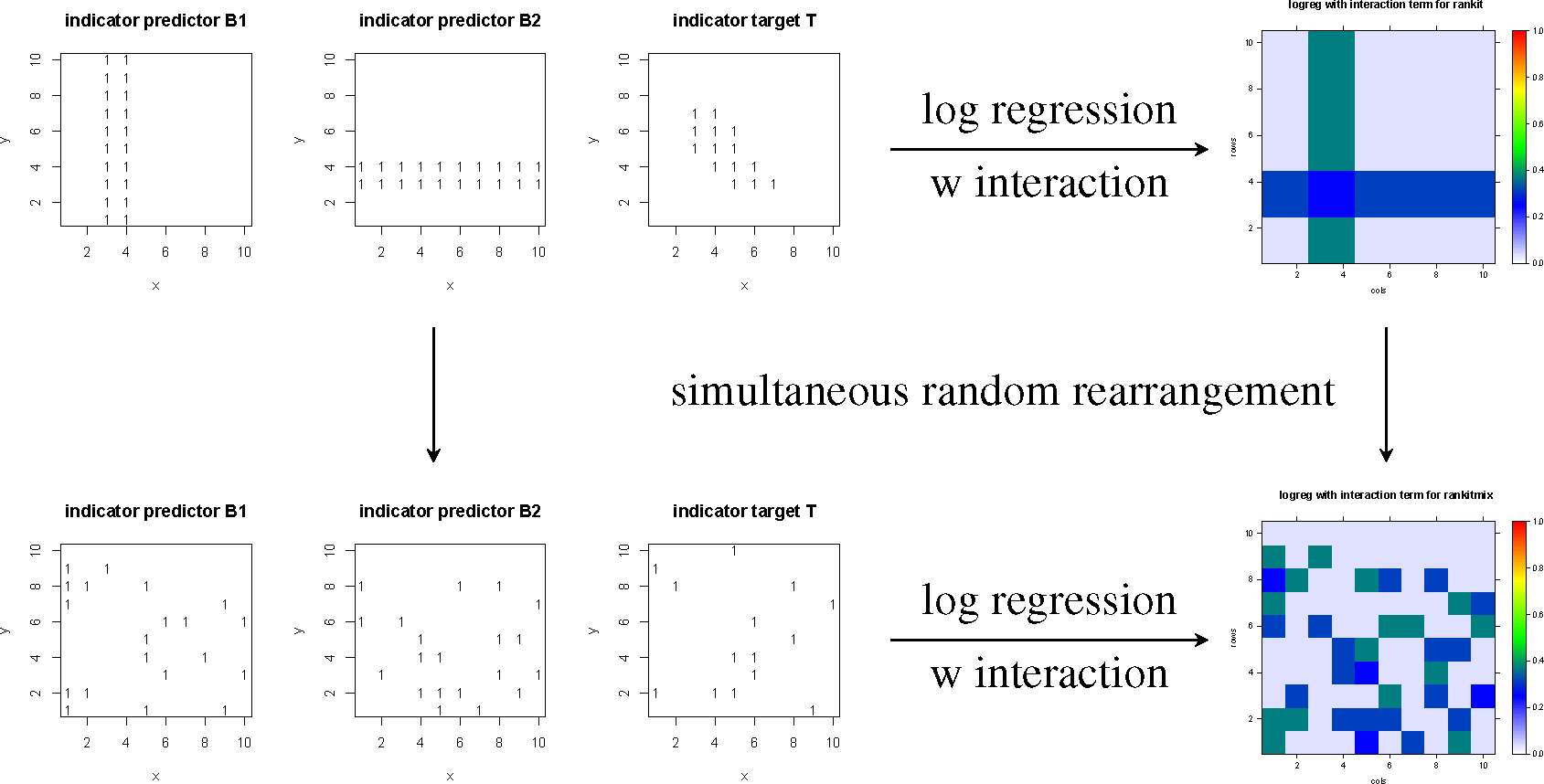
Obviously, the digital map images of Figures 2 and 3 are related to each other by the same rearrangement as the datasets rankit and rankitmix of the top row of Figure 1. This relationship can be depicted like a commutative diagram (Figure 4), for instance with respect to logistic regression, including interaction terms.

To state it explicitly, each of the methods of targeting considered here commutes with any random rearrangement applied simultaneously to all digital map images involved in or resulting from targeting. Thus, targeting and potential modeling, resp., are not spatial methods; they do not employ spatially-induced dependencies, which have been shown to be different by looking at the semi-variograms of the datasets; Figure 1.

After balancing with m = 10, the models of weights-of-evidence and enlarged logistic regression with interaction terms read explicitly:

$$\begin{array}{cc}\hfill \mathrm{WofE}:& \widehat{P}({\mathrm{T}}^{\mathrm{bal}}=1|{\mathrm{B}}_1^{\mathrm{bal}}{\mathrm{B}}_2^{\mathrm{bal}})=\mathrm{\Lambda }\left(-0.423+1.725{\mathrm{B}}_1^{\mathrm{bal}}+1.349{\mathrm{B}}_2^{\mathrm{bal}}\right)\hfill \\ \hfill \mathrm{logRegwI}:& \widehat{P}({\mathrm{T}}^{\mathrm{bal}}=1|{\mathrm{B}}_1^{\mathrm{bal}}{\mathrm{B}}_2^{\mathrm{bal}})=\mathrm{\Lambda }(-1.132+2.923{\mathrm{B}}_1^{\mathrm{bal}}+2.646{\mathrm{B}}_2^{\mathrm{bal}}-3.233{\mathrm{B}}_1^{\mathrm{bal}}{\mathrm{B}}_2^{\mathrm{bal}})\hfill \end{array}$$

with −0.423 − ln(10) = −0.423 − 2.302 = −2.726 and −1.132 − 2.302 = −3.434, respectively, thus confirming Equation (11). However, the ordinary logistic regression model without interaction terms reads:

$$\begin{array}{cc}\mathrm{ologReg}:& \widehat{P}({\mathrm{T}}^{\mathrm{bal}}=1|{\mathrm{B}}_1^{\mathrm{bal}}{\mathrm{B}}_2^{\mathrm{bal}})=\mathrm{\Lambda }(-0.960+2.468{\mathrm{B}}_1^{\mathrm{bal}}+2.201{\mathrm{B}}_2^{\mathrm{bal}})\end{array}$$

with −0.960 − 2.302 = −3.263 ≠ −2.831 and different parameters ${\beta }_1^{\mathrm{bal}}$ and ${\beta }_2^{\mathrm{bal}}$, as the ordinary logistic regression model is not a proper model due to the violation of the modeling assumption of conditional independence.

3.2. Dataset DFQR

The dataset DFQR is visualized as a digital map image in Figure 5.

The contingencies are given in

Table 5. Unconditional contingency table of B₁ and B₂, and conditional contingency tables of B₁ and B₂ given T of dataset DFQR.

	B2 = 0	B2 = 1
B1 = 0	64	15
B1 = 1	15	6

T = 0	B2 = 0	B2 = 1
B1 = 0	60	11
B1 = 1	11	2

T = 1	B2 = 0	B2 = 1
B1 = 0	4	4
B1 = 1	4	4

and

Table 6. Contingency tables of T and B₁ and B₂, respectively, of dataset DFQR.

	B1 = 0	B1 = 1
T= 0	71	13
T= 1	8	8

	B2 = 0	B2 = 1
T= 0	71	13
T= 1	8	8

.

The correlation matrix (

Table 7. Correlation matrix of dataset of dataset DFQR.

	B1	B2	T
B1	1.0000000	0.0958409	0.3107386
B2	0.0958409	1.0000000	0.3107386
T	0.3107386	0.3107386	1.0000000

) indicates that B₁ and B₂ are uncorrelated, and significantly correlated with T for all significance levels α > 0.001652.

The test of conditional independence referring to log-linear models (

Table 8. Significance test of the null-hypothesis of conditional independence, referring to a log-linear model for dataset DFQR.

Statistics
	χ2	df	P(> χ2)
Likelihood Ratio	9.872996e-05	2	0.9999506
Pearson	9.859977e-05	2	0.9999507

) shows that the null-hypothesis of conditional independence of B₁ and B₂ given T cannot reasonably be rejected.

The corresponding conditional relative frequencies factorize almost exactly, i.e.,

$$P\left(B_1=1,B_2=1|\mathrm{T}=1\right)=P\left(B_1=1|\mathrm{T}=1\right)P\left(B_2=1|\mathrm{T}=1\right)=0.25$$

but:

$$P\left(B_1=1,B_2=1|\mathrm{T}=0\right)=0.02380952$$

and:

$$P\left(B_1=1|\mathrm{T}=0\right)P\left(B_2=1|\mathrm{T}=0\right)=0.02395125$$

With $\widehat{\mathrm{O}}\left(\mathrm{T}=1\right)=0.1904,\log \mathrm{it}\widehat{P}\left(\mathrm{T}=1\right)=-1.6582$, the weights-of-evidence model reads explicitly:

$$\widehat{P}\left(\mathrm{T}=1|{\mathrm{B}}_1{\mathrm{B}}_2\right)=\mathrm{\Lambda }\left(-2.7082+1.6977{\mathrm{B}}_1+1.6977{\mathrm{B}}_2\right)$$

The ordinary logistic regression model without interaction terms reads explicitly:

$$\widehat{P}\left(\mathrm{T}=1|{\mathrm{B}}_1{\mathrm{B}}_2\right)=\mathrm{\Lambda }\left(-2.7094+1.6994{\mathrm{B}}_1+1.6994{\mathrm{B}}_2\right)$$

where:

• β₀ is significant for all α > 1.12e − 08, and

• β₁, β₂ are significant for all α > 0.00651.

The two models are almost identical; small deviations of their parameters result from small violations of conditional independence. While the test with p = 0.999950 indicates that the null-hypothesis of conditional independence cannot reasonable be rejected, the conditional relative frequencies do not factorize perfectly, but only approximately. The conditional probabilities estimated with weights-of-evidence or ordinary logistic regression almost exactly recover the conditional probabilities estimated elementarily by counting conditional frequencies for the training dataset DFQR; cf.

Table 9. Comparison of conditional probabilities predicted with elementary counting, weights-of-evidence (WofE), ordinary logistic regression without interaction terms (oLogReg), logistic regression including interaction terms (LogRegwI), and artificial neural nets using a genetic algorithm (ANNGA [38]) applied to the training dataset DFQR.

$\widehat{P}\left(T=1|B_1{B}_2\right)$	Counting	WofE	oLogReg	LogRegwI	ANNGA
B1 = 1, B2 = 1	0.66666	0.66534	0.66585	0.66666	0.66666
B1 = 1, B2 = 0	0.26666	0.26687	0.26699	0.26666	0.26666
B1 = 0, B2 = 1	0.26666	0.26687	0.26699	0.26666	0.26666
B1 = 0, B2 = 0	0.06250	0.06248	0.06242	0.06250	0.06250

.

The logistic regression model with interaction terms reads explicitly:

$$\widehat{P}\left(\mathrm{T}=1|{\mathrm{B}}_1{\mathrm{B}}_2\right)=\mathrm{\Lambda }\left(-2.7080+1.6964{\mathrm{B}}_1+1.6964{\mathrm{B}}_2+0.0082{\mathrm{B}}_1{\mathrm{B}}_2\right)$$

where:

• β₀ is significant for all α > 1.57e − 07,

• β₁, β₂ are significant for all α > 0.0295, and

• β₁₂ is not at all significant as p = 0.9949.

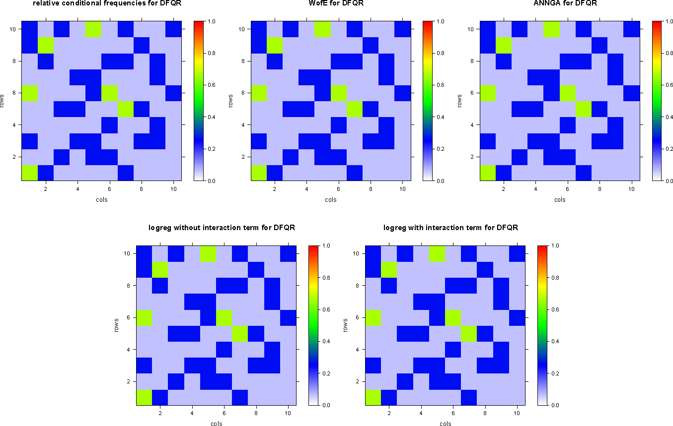
The conditional probabilities estimated with logistic regression, including the interaction terms, exactly recover the conditional probabilities estimated elementarily by counting conditional frequencies for the training dataset DFQR, which is just the numerical confirmation, that the log-linear model with interaction terms is a perfect model for the training dataset DFQR; cf. Table 9 and Figure 6.

After balancing with m = 10, the models for the balanced dataset are:

$$\begin{array}{cc}\hfill \mathrm{WofE}:& \widehat{P}({\mathrm{T}}^{\mathrm{bal}}=1|{\mathrm{B}}_1^{\mathrm{bal}}{\mathrm{B}}_2^{\mathrm{bal}})=\mathrm{\Lambda }(-0.4056+1.697{\mathrm{B}}_1^{\mathrm{bal}}+1.697{\mathrm{B}}_2^{\mathrm{bal}})\hfill \\ \hfill \mathrm{ologReg}:& \widehat{P}({\mathrm{T}}^{\mathrm{bal}}=1|{\mathrm{B}}_1^{\mathrm{bal}}{\mathrm{B}}_2^{\mathrm{bal}})=\mathrm{\Lambda }(-0.4059+1.698{\mathrm{B}}_1^{\mathrm{bal}}+1.698{\mathrm{B}}_2^{\mathrm{bal}})\hfill \\ \hfill \mathrm{logRegwI}:& \widehat{P}({\mathrm{T}}^{\mathrm{bal}}=1|{\mathrm{B}}_1^{\mathrm{bal}}{\mathrm{B}}_2^{\mathrm{bal}})=\mathrm{\Lambda }(-0.4054+1.696{\mathrm{B}}_1^{\mathrm{bal}}+1.696{\mathrm{B}}_2^{\mathrm{bal}}+0.008299{\mathrm{B}}_1^{\mathrm{bal}}{\mathrm{B}}_2^{\mathrm{bal}})\hfill \end{array}$$

confirming Equation (11), as the assumption of conditional independence was not rejected.

4. Conclusions

Targeting or potential modeling applies regression or regression-like models to estimate the conditional probability of a target variable given predictor variables. All models considered here:

• assume independently identical distributed random predictor and target variables, respectively, i.e., all models are non-spatial and do not consider spatially-induced dependencies, as, for instance, geostatistics; therefore, rearranging the dataset at random results in random map images or geomodels, but does not change the fitted models.

• are not pointwise; they involve random variables referring to locations given in terms of areal pixels of 2D digital map images or volumetric voxels of 3D geomodels; thus, their results depend on the spatial resolution of the map image or the geomodel, respectively.

• require a training region to fit the model parameters; that is to say that the mathematical modeling assumption associated with the training region is that it provides “ground truth”.

Then, the models can be put in a hierarchy, beginning with the naive Bayesian model of weights-of-evidence depending on the modeling assumption of conditional independence of all predictor variables given the target variable. It is the special case of the logistic regression model if the predictor variables (i) are indicator or discrete random variables and (ii) conditionally independent given the target variable. In this case, the contrasts of weights-of-evidence are identical to the logistic regression coefficients. Otherwise, there is no linear relationship between weights of evidence and logistic regression parameters.

The canonical generalization of the naive Bayesian model featuring weights of evidence to the case of lacking conditional independence is logistic regression, including interaction terms. If the interactions terms are chosen to correspond to violations of conditional independence, they are compensating exactly for these violations, if the predictor variables are discrete; for continuous predictor variables, they compensate exactly only if the joint probability is log-linear; otherwise, they may compensate approximately. Thus, in the case of discrete predictor variables, the logistic regression model is optimum.

Applying weights-of-evidence despite lacking conditional independence corrupts both the predicted conditional probabilities, as well as their rank-transforms. Their is no way to emulate the effect of interaction terms by “correcting” the weights of evidence subsequently, e.g., by powering or multiplying with some τ- or ν-coefficients.

To further enlarge the models, nesting logistic regression-like models is an option. Irrespective of the vocabulary, nesting giving rise to “hidden layers” is the hard core of artificial neural nets. If the configuration of the net topology is sufficiently versatile, artificial neural net models can compensate for the lack of conditional independence, much in the same way as logistic regression models, including interaction terms. When the odds of the target are too small, some “balancing” may be required. A simple balancing method was shown to leave the model parameters unchanged, if the model itself is proper.

The possibility to include interaction terms in logistic regression models or other models originating in statistical learning opens a promising route toward an effective means to abandon the severe modeling assumption of conditional independence and to cope with the lack of conditional independence in practice.

A promising future perspective is regression accounting for spatially-induced dependencies to get rid of (i) the training region partitioned in pixels or voxels and the dependence on the spatial resolution that they provide; and (ii) the modeling assumption of independently identical distributed random variables.

References

- Hronsky, J.M.A.; Groves, D.I. Science of targeting: Definition, strategies, targeting and performance measurement. Aust. J. Earth Sci. 2008, 55, 3–12. [Google Scholar]
- Cox, D.P.; Singer, D.A. Mineral Deposit Models; U.S. Geological Survey Bulletin 1693; US Government Printing Office: Washington, DC, USA, 1986. [Google Scholar]
- Chilès, J.-P.; Delfiner, P. Geostatistics—Modeling Spatial Uncertainty, 2nd ed.; John Wiley & Sons: Hoboken, NJ, USA, 2012. [Google Scholar]
- Independence and Conditional Independence, Available online: http://www.eecs.qmul.ac.uk/norman/BBNs/Independence_and_conditional_independence.htm accessed on 10 October 2014.
- Mitchell, T.M. Machine Learning; McGraw-Hill: New York, NY, USA, 1997. [Google Scholar]
- Højsgaard, S.; Edwards, D.; Lauritzen, S. Graphical Models with R.; Springer: New York, NY, USA, 2012. [Google Scholar]
- Schaeben, H. A mathematical view of weights-of-evidence, conditional independence, and logistic regression in terms of markov random fields. Math. Geosci. 2014, 46, 691–709. [Google Scholar]
- Hosmer, D.W.; Lemeshow, S. Applied Logistic Regression, 2nd ed.; Wiley: New York, NY, USA, 2000. [Google Scholar]
- Schaeben, H. Potential modeling: Conditional independence matters. Int. J. Geomath. 2014, 5, 99–116. [Google Scholar]
- Agterberg, F.P.; Bonham-Carter, G.F.; Wright, D.F. Statistical pattern integration for mineral exploration. In Computer Applications in Resource Estimation Prediction and Assessment for Metals and Petroleum; Gaál, G., Merriam, D.F., Eds.; Pergamon Press: Oxford, NY, USA, 1990; pp. 1–21. [Google Scholar]
- Bonham-Carter, G.F.; Agterberg, F.P. Application of a microcomputer based geographic information system to mineral-potential mapping. In Microcomputer—Based Applications in Geology II, Petroleum; Hanley, J.T., Merriam, D.F., Eds.; Pergamon Press: New York, NY, USA, 1990; pp. 49–74. [Google Scholar]
- Good, I.J. Probability and the Weighing of Evidence; Griffin: London, UK, 1950. [Google Scholar]
- Good, I.J. The Estimation of Probabilities: An Essay on Modern Bayesian Methods; Research Monograph No. 30; The MIT Press: Cambridge, MA, USA, 1968. [Google Scholar]
- Hand, D.J.; Yu, K. Idiot’s bayes—Not so stupid after all? Int. Stat. Rev. 2001, 69, 385–398. [Google Scholar]
- Hastie, T.; Tibshirani, R.; Friedman, J. The Elements of Statistical Learning; Springer: New York, NY, USA, 2001. [Google Scholar]
- Smola, A.J.; Vishwanathan, S.V.N. Introduction to Machine Learning; Cambridge University Press: Cambridge, UK, 2008. [Google Scholar]
- Sutton, C.; McCallum, A. An introduction to conditional random fields for relational learning. In Introduction to Statistical Relational Learning; Getoor, L., Taskar, B., Eds.; MIT Press: London, UK, 2007; pp. 93–127. [Google Scholar]
- Agterberg, F.P.; Cheng, Q. Conditional independence test for weights-of-evidence modeling. Nat. Resour. Res. 2002, 11, 249–255. [Google Scholar]
- Bonham-Carter, G.F. Geographic Information Systems for Geoscientists; Pergamon Press: Oxford, NY, USA, 1994. [Google Scholar]
- Zhang, K.; Peters, J.; Janzing, D.; Schölkopf, B. Kernel-based conditional independence test and application in causal discovery, Proceedings of the 27th Conference on Uncertainty in Artificial Intelligence (UAI 2011), Barcelona, Spain, 14–17 July 2011; Cozman, F.G., Pfeffer, A., Eds.; AUAI Press: Corvallis, OR, USA, 2011; pp. 804–813.
- Schaeben, H. Comparison of mathematical methods of potential modeling. Math. Geosci. 2012, 44, 101–129. [Google Scholar]
- Schaeben, H.; van den Boogaart, K.G. Comment on “A conditional dependence adjusted weights of evidence model” by Minfeng Deng in Natural Resources Research 18(2009), 249–258. Nat. Resour. Res. 2011, 29, 401–406. [Google Scholar]
- Journel, A.G. Combining knowledge from diverse sources: An alternative to traditional data independence hypotheses. Math. Geol. 2002, 34, 573–596. [Google Scholar]
- Krishnan, S.; Boucher, A.; Journel, A.G. Evaluating information redundancy through the τ-model. In Geostatistics Banff 2004; Leuangthong, O., Deutsch, C.V., Eds.; Springer: Dordrecht, The Netherlands, 2005; pp. 1037–1046. [Google Scholar]
- Krishnan, S. The τ-model for data redundancy and information combination in earth sciences: Theory and Application. Math. Geosci. 2008, 40, 705–727. [Google Scholar]
- Polyakova, E.I.; Journel, A.G. The ν-model for probabilistic data integration, IAMG’2006, Proceedings of the XIth International Congress of the International Association for Mathematical Geology: Quantitative Geology from Multiple Sources, Liège, Belgium, 3–8 September 2006.
- Polyakova, E.I.; Journel, A.G. The ν-expression for probabilistic data integration. Math. Geol. 2007, 39, 715–733. [Google Scholar]
- Vapnik, V.N. The Nature of Statistical Learning Theory, 2nd ed.; Springer: New York, NY, USA, 2000. [Google Scholar]
- Bishop, C.M. Pattern Recognition and Machine Learning; Springer: New York, NY, USA, 2006. [Google Scholar]
- Russell, S.; Norvig, P. Artificial Intelligence, A Modern Approach, 2nd ed.; Prentice Hall: Upper Saddle River, NJ, USA, 2003. [Google Scholar]
- Skabar, A. Modeling the spatial distribution of mineral deposits using neural networks. Nat. Resour. Model. 2007, 20, 435–450. [Google Scholar]
- Adam, A.; Ibrahim, Z.; Shapiai, M.I.; Chew, L.C.; Jau, L.W.; Khalid, M.; Watada, J. A two-stwp supervised learning artificial neural network for imbalanced dataset problems. Int. J. Innov. Comput. Inf. Control. 2012, 8, 3163–3172. [Google Scholar]
- Adam, A.; Shapiai, M.I.; Ibrahim, Z.; Khalid, M.; Jau, L.W. development of a hybrid artificial neural network—Naive bayes classifier for binary classification problem of imbalanced datasets. ICIC Express Lett. 2011, 5, 3171–3175. [Google Scholar]
- Batista, G.E.A.P.A.; Prati, R.C.; Monard, M.C. A study of the behavior of several methods for balancing machine learning training data. SIGKDD Explor. Spec. Issue Learn. Imbalanced Datasets. 2004, 6, 20–29. [Google Scholar]
- Chawla, N.V.; Bowyer, K.W.; Hall, L.O.; Kegelmeyer, W.P. Smote: Synthetic minority over-sampling technique. J. Artif. Intell. Res. 2002, 16, 321–357. [Google Scholar]
- Kotsiantis, S.; Kanellopoulos, D.; Pintelas, P. Handling imbalanced datasets: A review. GESTS Int. Trans. Comput. Sci. Eng. 2006, 30, 25–36. [Google Scholar]
- Zhao, Z.-Q. A novel modular neural network for imbalanced classification problems. Pattern Recognit. Lett. 2008, 30, 783–788. [Google Scholar]
- R Development Core Team. R—A Language and Environment for Statistical Computing; R Foundation for Statistical Computing: Vienna, Austria, 2013. Available online: http://www.R-project.org/ accessed on 10 October 2014.