
Spatial Air Index Based on Largest Empty Rectangles for Non-Flat Wireless Broadcast in Pervasive Computing


Abstract
:1. Introduction
- For processing window queries, the information about the largest empty rectangle of the cells is provided in the spatial air index to further bound the search region and skip irrelevant broadcast content, thus reducing access and tuning times.
- Various experiments with different settings verify the effectiveness of the proposed spatial air index method, which outperforms the existing methods SSI and MLAIN.
2. Related Work
2.1. Flat Data Broadcast
2.2. Non-Flat Data Broadcast
3. Proposed Spatial Air Index Method
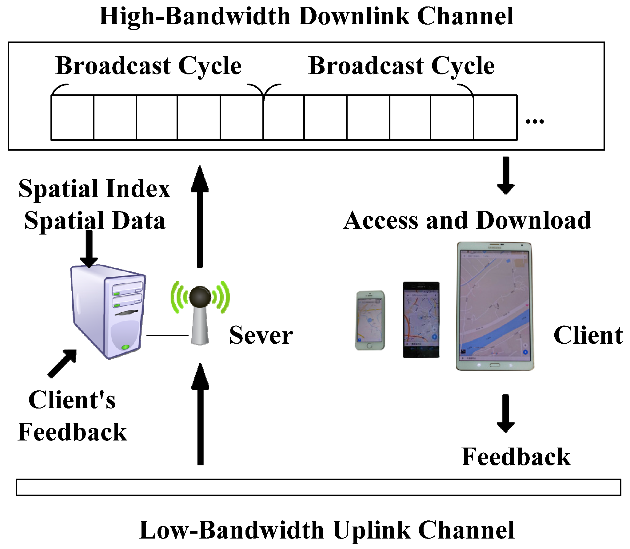
3.1. System Model
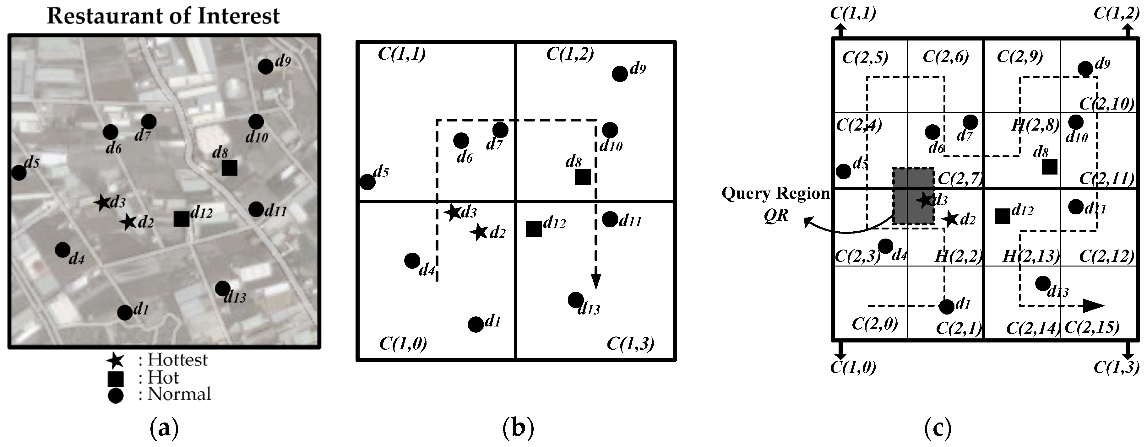
3.2. Mapping of Spatial Data from 2D to 1D
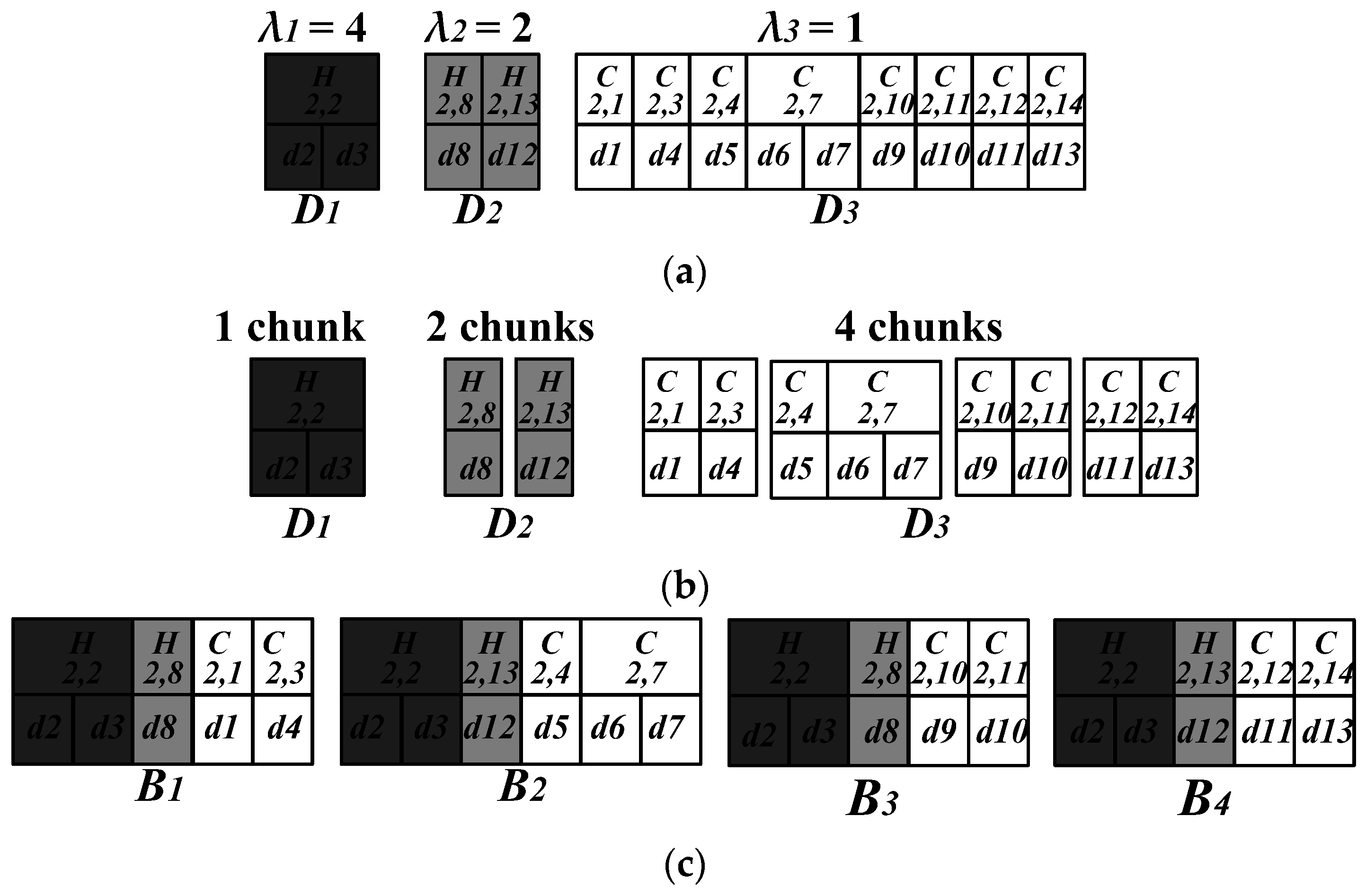
3.3. Generation of the Non-Flat Broadcast Program
3.4. Construction of the Index Structure and Largest Empty Rectangles
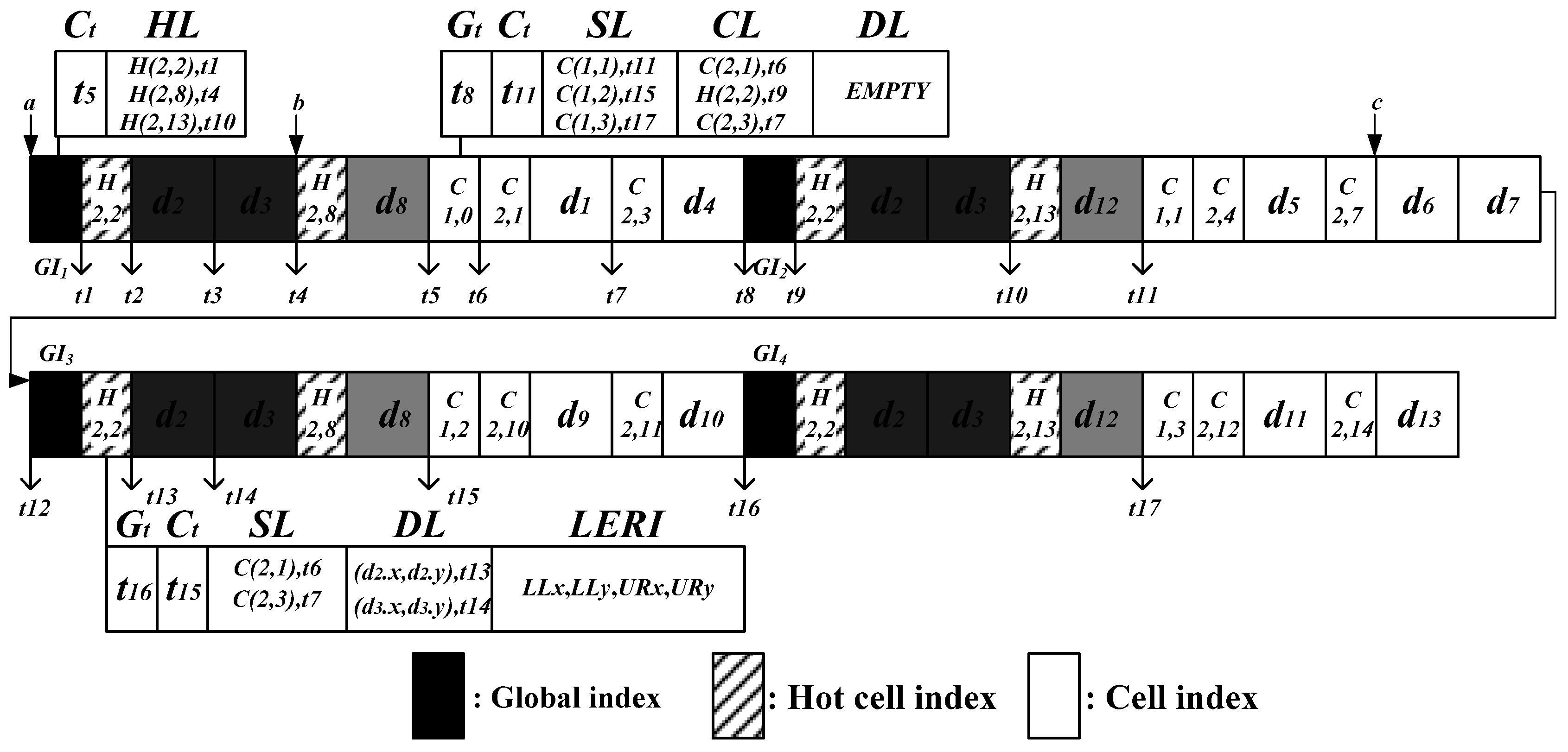
- Global index: G = <Ct, HL>
- Ct is the arrival time of the nearest upcoming cell index of Level 1 in the wireless channel. For example, Ct in the first global index in Figure 5 points to the beginning of cell index C(1,0), t5.
- HL contains the arrival time of the cell indexes for all hot cells. For example, HL in the first global index in Figure 5 contains information about all the hot cells, H(2,2), H(2,8) and H(2,13).
- Hot cell index: H(i,j) = <Gt, Ct, SL, DL, LERI>
- Gt is the arrival time of the nearest upcoming global index. For example, in Figure 5, Gt in the hot cell index of H(2,2) in the second row points to the beginning of the upcoming global index, t16.
- SL contains information about the sibling cells of the same level.
- DL contains the coordinates of the spatial objects in that cell, and their corresponding arrival times. From DL, the mobile device can determine whether the spatial objects are contained within the query region before retrieving them from the channel.
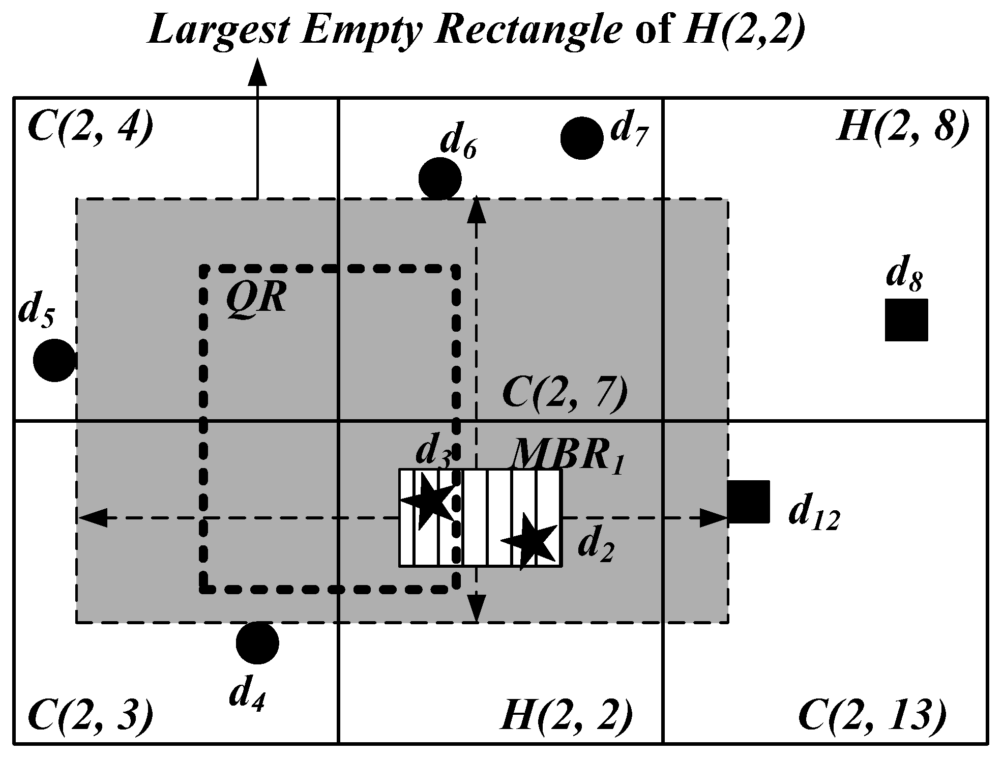
- LERI represents the information about the largest empty rectangle of this hot cell. The lower-left and upper-right coordinates of the largest empty rectangle are recorded in LERI.
- Cell index: C(i,j) = <Gt, Ct, SL, CL, DL>
- CL contains information about the corresponding child cells of the next level. For example, in Figure 5, CL in the cell index of C(1,0) of Level 1 contains information about the child cells of Level 2, C(2,1), H(2,2), and C(2,3).
3.5. Access Processing for Window Queries
| Algorithm 1. Process a Window Query |
| Input: Examination set ES. |
| Output: The relevant objects. |
|
4. Simulation Study
4.1. Simulation Model
4.2. Simulation Results
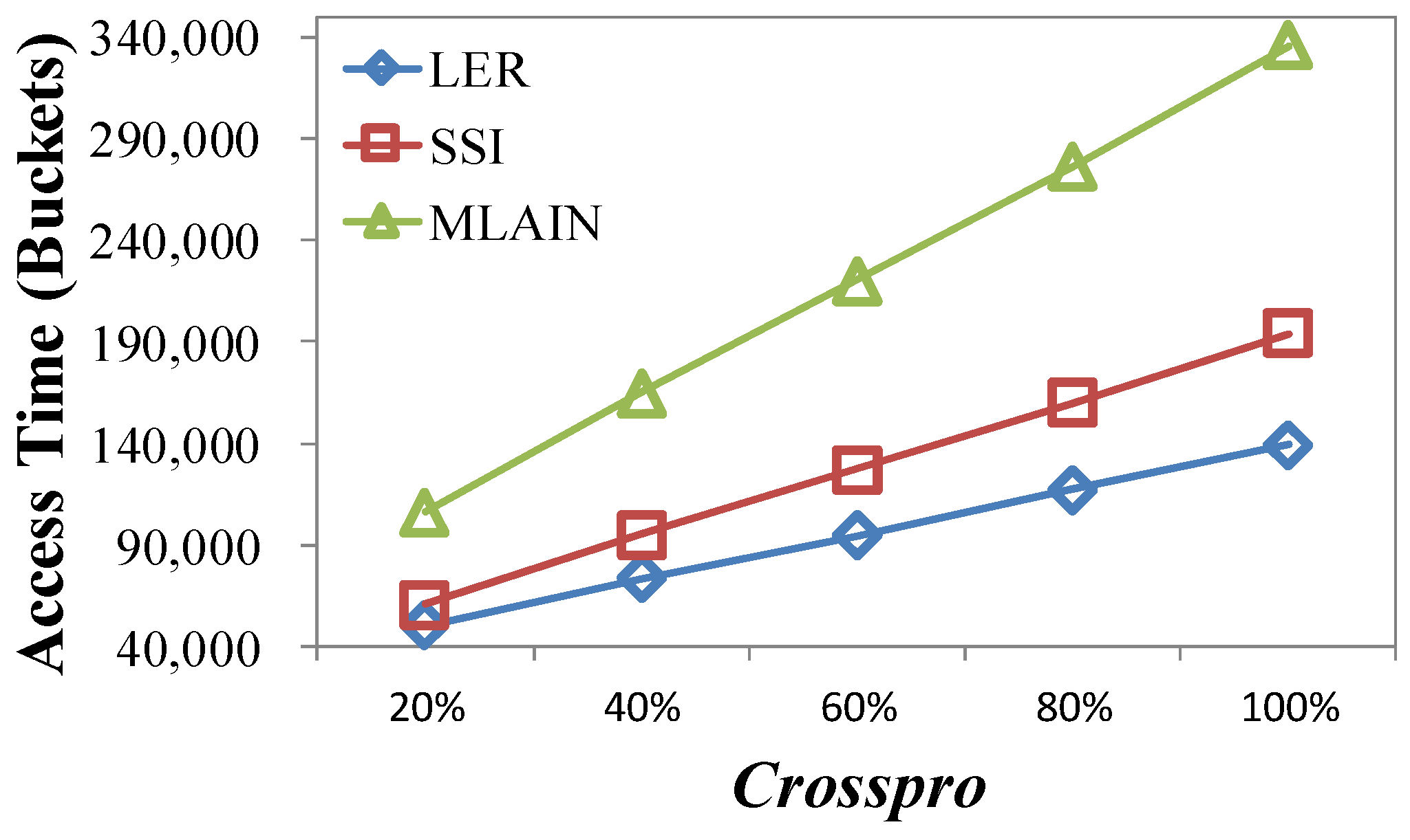
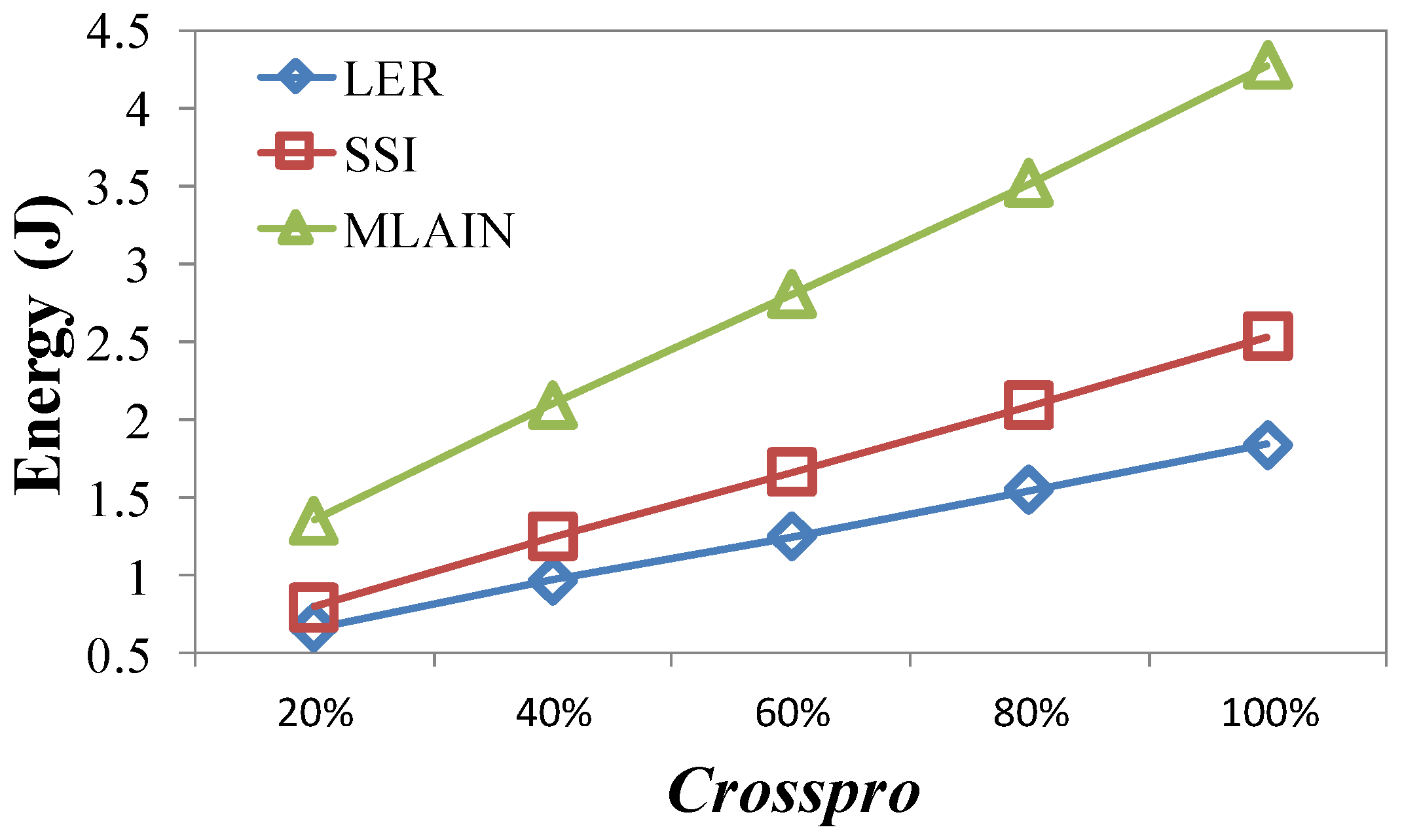
4.2.1. Impact of Crosspro
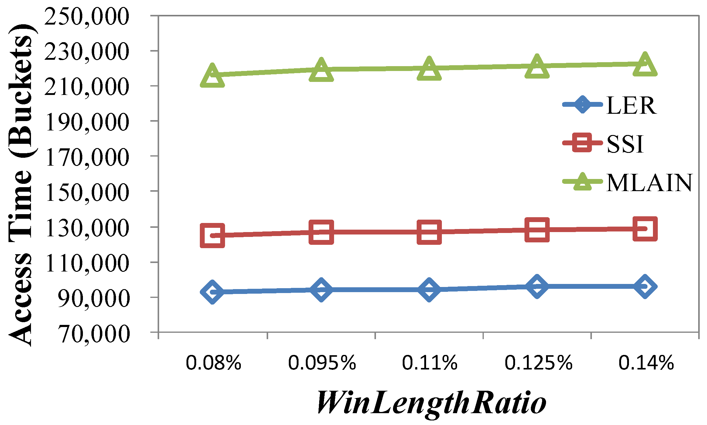
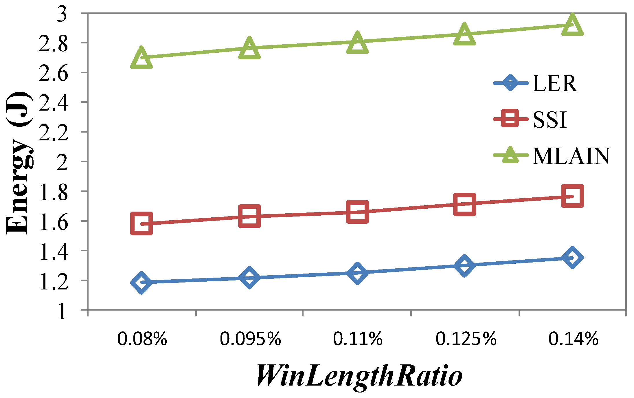
4.2.2. Impact of WinLengthRatio
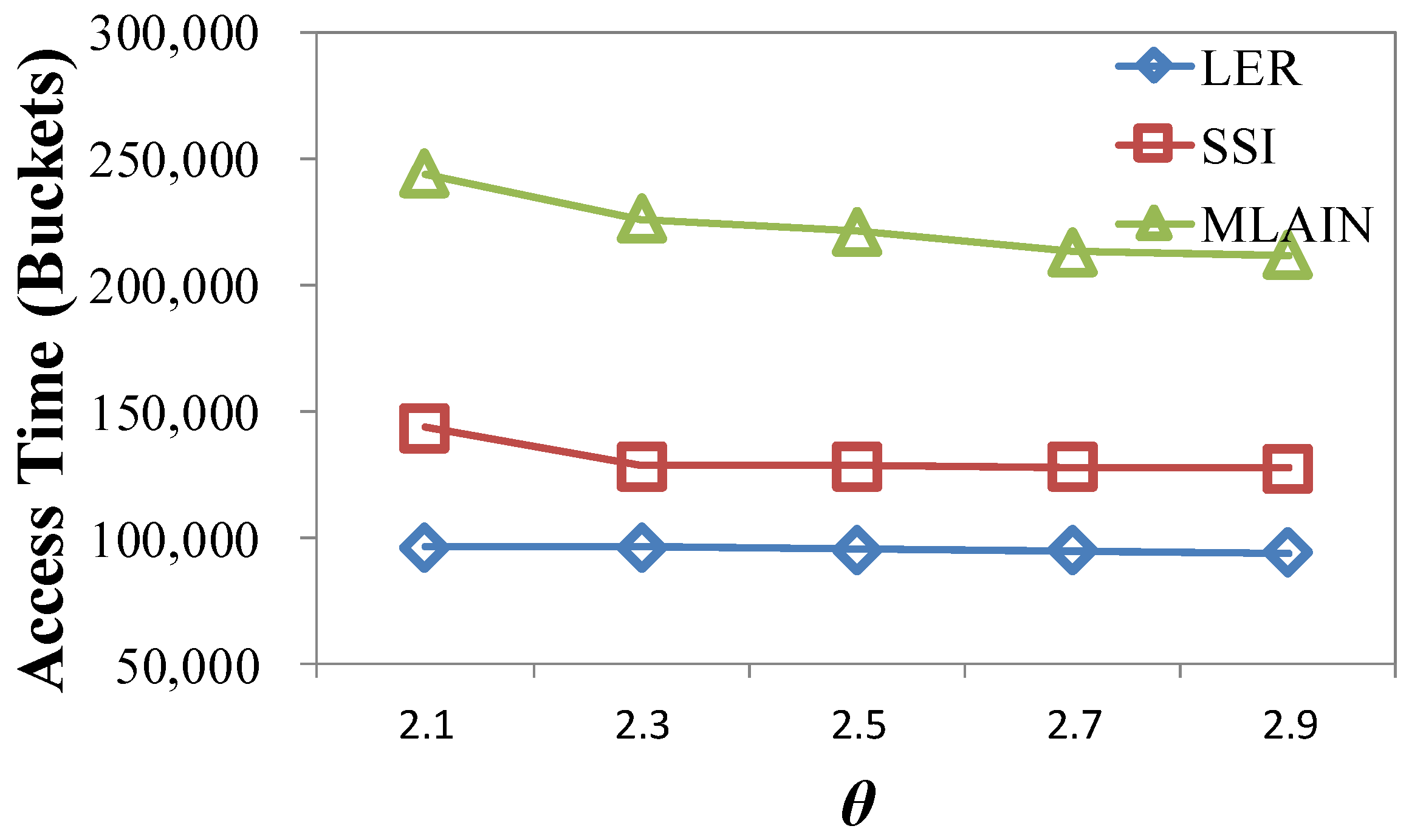
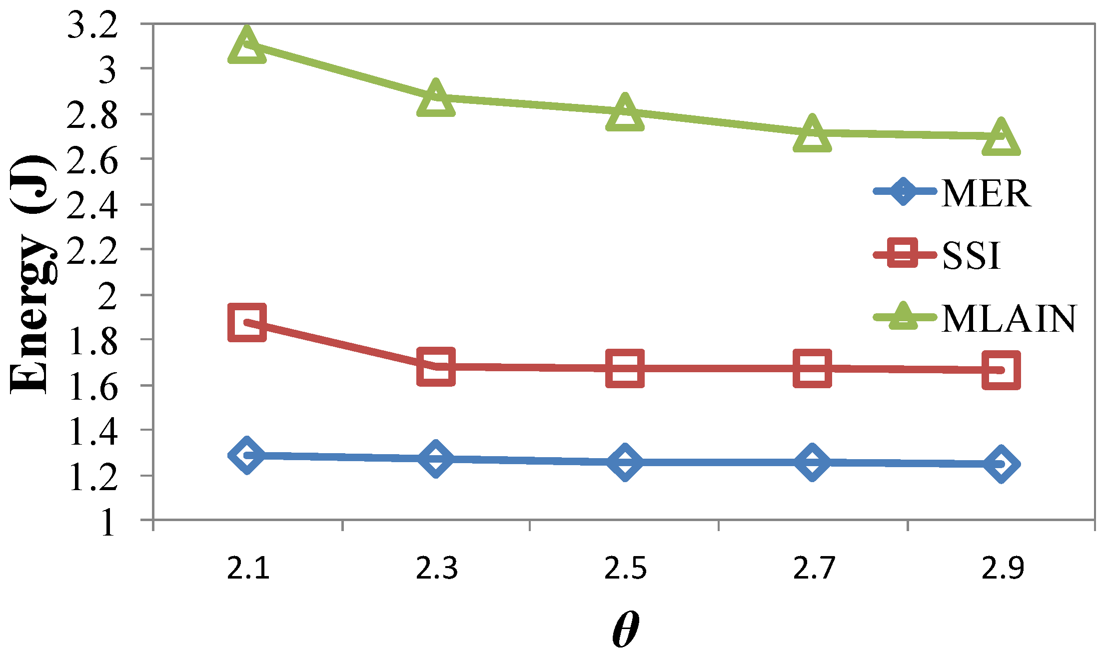
4.2.3. Impact of θ
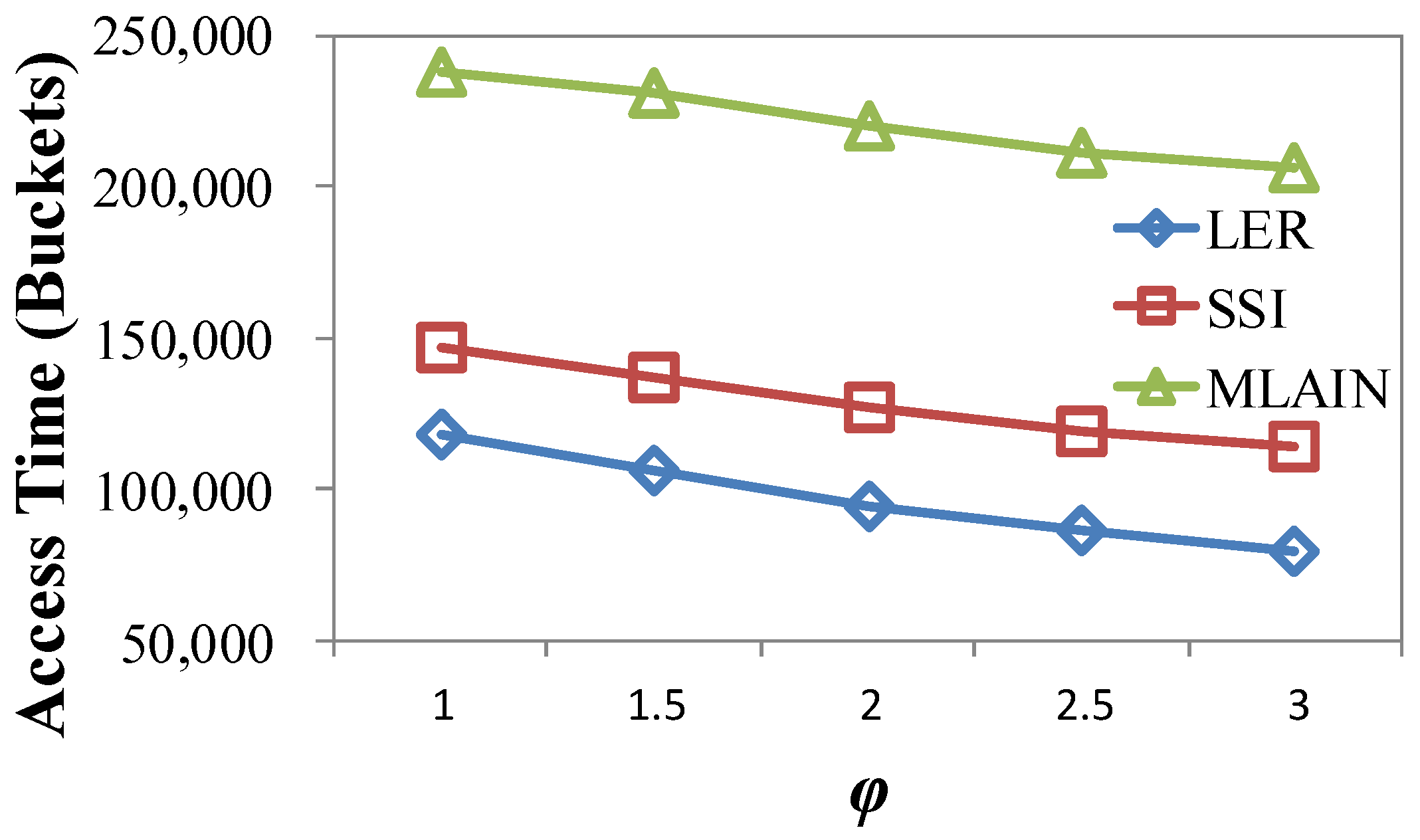
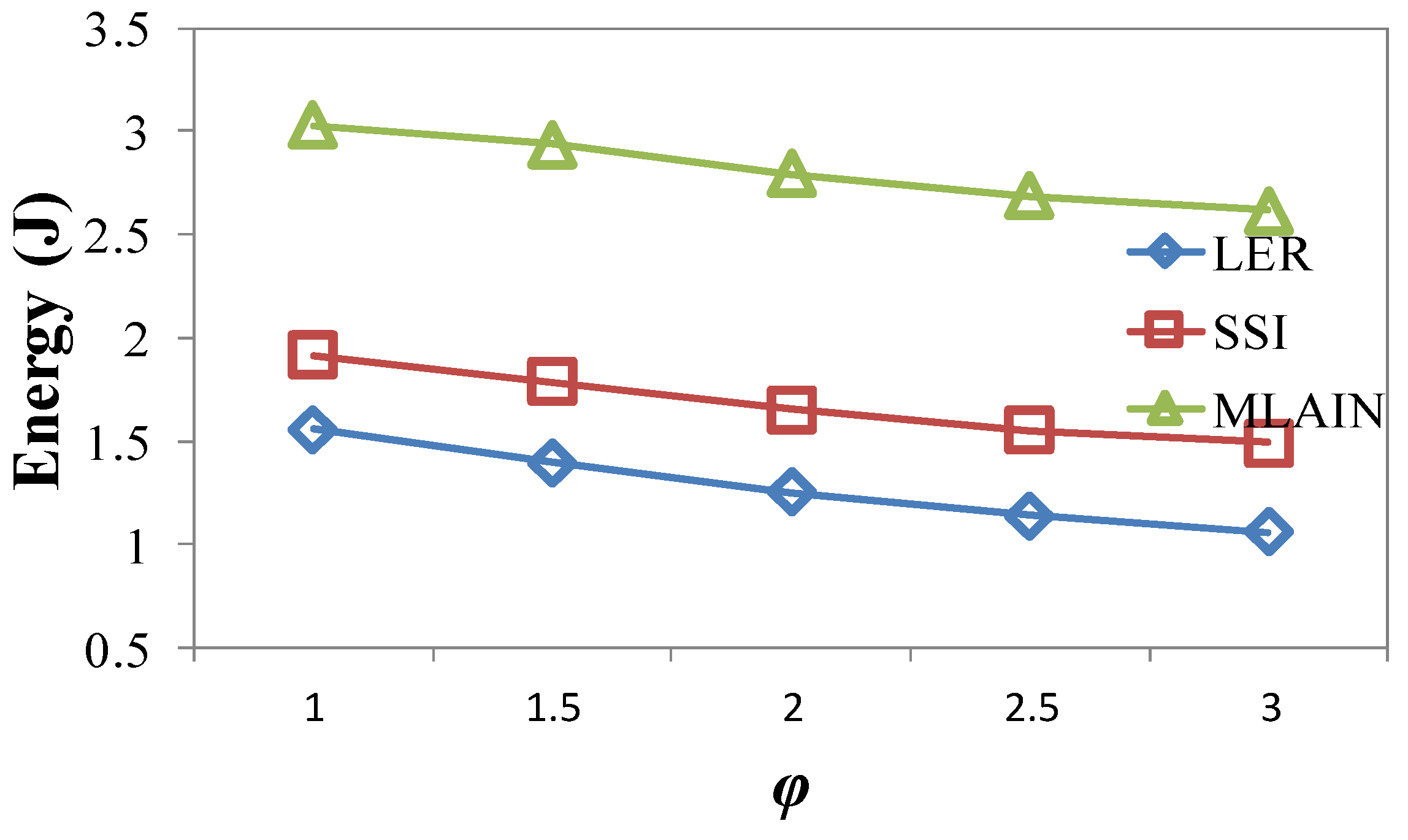
4.2.4. Impact of φ
5. Conclusions
Acknowledgments
Author Contributions
Conflicts of Interest
References
- Shen, J.H.; Lu, C.T.; Jian, M.S.; Huang, T.C. A skewed spatial index for continuous window queries in the wireless broadcast environments. Lect. Notes Elect. Eng. 2013, 253, 702–715. [Google Scholar]
- Shen, J.H.; Lu, C.T.; Jian, M.S. Neighbor-index method for continuous window queries over wireless. Appl. Mech. Mater. 2013, 284, 3295–3299. [Google Scholar] [CrossRef]
- Dhanked, S.; Goel, V. Hashing techniques for broadcasting in wireless data environment. In Proceedings of the International Conference on Issues and Challenges in Intelligent Computing Techniques, Ghaziabad, India, 7–8 February 2014.
- Gao, X.; Yang, Y.; Chen, G.; Lu, X. Global optimization for multi-channel wireless data broadcast with AH-tree indexing scheme. IEEE Trans. Comput. 2016, 65, 2104–2117. [Google Scholar] [CrossRef]
- Goel, V.; Ahalawat, A.K.; Gupta, M.N. Distributed air indexing scheme for full-text search on multiple wireless channel. In Intelligent Systems Technologies and Applications; Berretti, S., Thampi, S.M., Dasgupta, S., Eds.; Springer: Berlin, Germany, 2016; pp. 125–135. [Google Scholar]
- Vishnoi, S.; Goel, V. Novel table based air indexing technique for full text search. In Proceedings of the International Conference on Computational Intelligence and Communication Technology, Ghaziabad, India, 13–14 February 2015.
- Zhong, J.; Wu, W.; Gao, X.; Shi, Y.; Yue, X. Evaluation and comparison of various indexing schemes in single-channel broadcast communication environment. Knowl. Inf. Syst. 2014, 40, 375–409. [Google Scholar] [CrossRef]
- Rakotonirainy, A.; Obst, P.; Loke, S.W. Socially aware computing constructs. Int. J. Soc. Humanist. Comput. 2012, 1, 375–395. [Google Scholar] [CrossRef]
- Acharya, S.; Franklin, M.; Zdonik, S.; Alongso, R. Broadcast disks: Data management for asymmetric communications environments. In Proceedings of the 1995 ACM SIGMOD International Conference on Management of Data, San Jose, CA, USA, 22–25 May 1995.
- Shen, J.H.; Chang, Y.I. A skewed distributed indexing for skewed access patterns on the wireless broadcast. J. Syst. Softw. 2007, 80, 711–723. [Google Scholar] [CrossRef]
- Im, S.; Joo, K.H.; Choi, J. Efficient windows query processing with expanded grid cells on wireless spatial data broadcasting for pervasive computing. Contemp. Eng. Sci. 2014, 7, 785–790. [Google Scholar] [CrossRef]
- Park, K.; Valduriez, P. A hierarchical grid index (HGI), spatial queries in wireless data broadcasting. Distrib. Parallel Databases 2013, 31, 413–446. [Google Scholar] [CrossRef]
- Park, K. An efficient scalable spatial data search for location-aware mobile services. J. Inf. Sci. Eng. 2015, 31, 165–178. [Google Scholar]
- Jung, S.; Mo, H. A spatial indexing scheme for location based service queries in a single wireless broadcast channel. J. Inf. Sci. Eng. 2014, 30, 1945–1963. [Google Scholar]
- Shen, J.H.; Chang, Y.I. An efficient nonuniform index in the wireless broadcast environments. J. Syst. Softw. 2008, 81, 2091–2103. [Google Scholar] [CrossRef]
- Song, D.; Park, K. A partial index for distributed broadcasting in wireless mobile networks. Inf. Sci. 2016, 348, 142–152. [Google Scholar] [CrossRef]
- Im, S.; Choi, J. MLAIN: Multi-leveled air indexing scheme in non-flat wireless data broadcast for efficient window query processing. Comput. Math. Appl. 2012, 64, 1242–1251. [Google Scholar] [CrossRef]
- Shen, J.H.; Jian, M.S. Spatial query processing for skewed access patterns in nonuniform wireless data broadcast environments. Int. J. Ad Hoc Ubiquitous Comput. 2016, in press. [Google Scholar]
- Aggarwal, A.; Suri, S. Fast algorithms for computing the largest empty rectangle. In Proceedings of the Third Annual Symposium on Computational Geometry, Waterloo, ON, Canada, 8–10 June 1987.
- Shen, J.H.; Lu, C.T.; Mai, C.T. Efficient processing of spatial window queries for non-flat wireless broadcast. In Proceedings of the 5th International Conference on Frontier Computing, Tokyo, Japan, 13–15 July 2016.
- Im, S.; Youn, H.Y.; Choi, J.; Ouyang, J. A novel air indexing scheme for window query in non-flat wireless spatial data broadcast. J. Commun. Net. 2011, 13, 400–407. [Google Scholar] [CrossRef]
- Zheng, B.; Lee, W.C.; Lee, C.K.; Lee, D.L.; Shao, M. A distributed spatial index for error-prone wireless data broadcast. VLDB J. 2009, 18, 959–986. [Google Scholar] [CrossRef]
- Vaidya, N.H.; Hameed, S. Scheduling data broadcast in asymmetric communication environments. Wirel. Net. 1999, 5, 171–182. [Google Scholar] [CrossRef]
- Zheng, B.; Lee, W.C.; Lee, D.L. Spatial queries in wireless broadcast systems. Wirel. Net. 2004, 10, 723–736. [Google Scholar] [CrossRef]
- Lee, W.; Zheng, B. DSI: A fully distributed spatial index for location-based wireless broadcast services. In Proceedings of the IEEE International Conference on Distributed Computing Systems (ICDCS), Columbus, OH, USA, 6–10 June 2005.
- Im, M.; Song, J.; Kim, S.K.; Hwang, C. An error-resilient cell-based distributed index for location-based wireless broadcast services. In Proceedings of the 5th ACM International Workshop on Data Engineering for Wireless and Mobile Access, Chicago, IL, USA, 25–28 June 2006.
- Im, S.; Hwang, H. A two-tier spatial index for non-flat spatial data broadcasting on air. IEICE Trans. Commun. 2014, 97, 2809–2818. [Google Scholar] [CrossRef]
- Yee, W.G.; Navathe, S.B.; Omiecinski, E. Efficient data allocation over multiple channels at broadcast servers. IEEE Trans. Comput. 2002, 51, 1231–1236. [Google Scholar]


| Parameter | Default Value | Meaning |
|---|---|---|
| θ | 2.5 | The Zipf factor to control the access skewness of the distribution of spatial objects |
| φ | 2 | The Zipf factor to control the access skewness of the distribution of disks |
| WinLengthRatio | 0.11% | The ratio of the side length of the query region to that of a map |
| Crosspro | 60% | The probability that a query region is crossing more than one cell |
| Crosspro | LER | SSI | MLAIN |
|---|---|---|---|
| 20% | 83.63 | 87.56 (4%) | 87.72 (5%) |
| 40% | 123.56 | 133.51 (7%) | 133.76 (8%) |
| 60% | 160.70 | 176.85 (9%) | 177.19 (9%) |
| 80% | 201.04 | 222.46 (10%) | 222.91 (10%) |
| 100% | 238.93 | 267.23 (11%) | 267.76 (11%) |
| WinLengthRatio | LER | SSI | MLAIN |
|---|---|---|---|
| 0.08% | 77.20 | 87.64 (12%) | 87.77 (12%) |
| 0.095% | 117.68 | 130.36 (10%) | 130.52 (10%) |
| 0.11% | 161.68 | 177.67 (9%) | 178.03 (9%) |
| 0.125% | 224.40 | 245.50 (9%) | 246.95 (9%) |
| 0.14% | 310.58 | 337.48 (8%) | 339.58 (9%) |
| θ | LER | SSI | MLAIN |
|---|---|---|---|
| 2.1 | 182.65 | 201.82 (9%) | 202.21 (10%) |
| 2.3 | 162.77 | 178.73 (9%) | 179.05 (9%) |
| 2.5 | 162.31 | 178.12 (9%) | 178.47 (9%) |
| 2.7 | 159.38 | 177.73 (11%) | 178.07 (11%) |
| 2.9 | 158.88 | 176.76 (10%) | 177.10 (10%) |
| φ | LER | SSI | MLAIN |
|---|---|---|---|
| 1 | 185.62 | 199.99 (7%) | 200.54 (7%) |
| 1.5 | 173.56 | 189.16 (8%) | 189.61 (8%) |
| 2 | 161.77 | 177.74 (9%) | 178.09 (9%) |
| 2.5 | 150.24 | 166.36 (10%) | 166.61 (10%) |
| 3 | 142.98 | 159.07 (10%) | 159.25 (10%) |
© 2016 by the authors; licensee MDPI, Basel, Switzerland. This article is an open access article distributed under the terms and conditions of the Creative Commons Attribution (CC-BY) license (http://creativecommons.org/licenses/by/4.0/).
Share and Cite
Shen, J.-H.; Lu, C.-T.; Chen, M.-Y.; Mai, C.-T. Spatial Air Index Based on Largest Empty Rectangles for Non-Flat Wireless Broadcast in Pervasive Computing. ISPRS Int. J. Geo-Inf. 2016, 5, 211. https://0-doi-org.brum.beds.ac.uk/10.3390/ijgi5110211
Shen J-H, Lu C-T, Chen M-Y, Mai C-T. Spatial Air Index Based on Largest Empty Rectangles for Non-Flat Wireless Broadcast in Pervasive Computing. ISPRS International Journal of Geo-Information. 2016; 5(11):211. https://0-doi-org.brum.beds.ac.uk/10.3390/ijgi5110211
Chicago/Turabian StyleShen, Jun-Hong, Ching-Ta Lu, Mu-Yen Chen, and Chien-Tang Mai. 2016. "Spatial Air Index Based on Largest Empty Rectangles for Non-Flat Wireless Broadcast in Pervasive Computing" ISPRS International Journal of Geo-Information 5, no. 11: 211. https://0-doi-org.brum.beds.ac.uk/10.3390/ijgi5110211