New Geospatial Approaches for Efficiently Mapping Forest Biomass Logistics at High Resolution over Large Areas


Abstract
:
1. Introduction
Comparison of Vector and Raster Methods
2. Materials and Methods
2.1. Case Study and Area Description
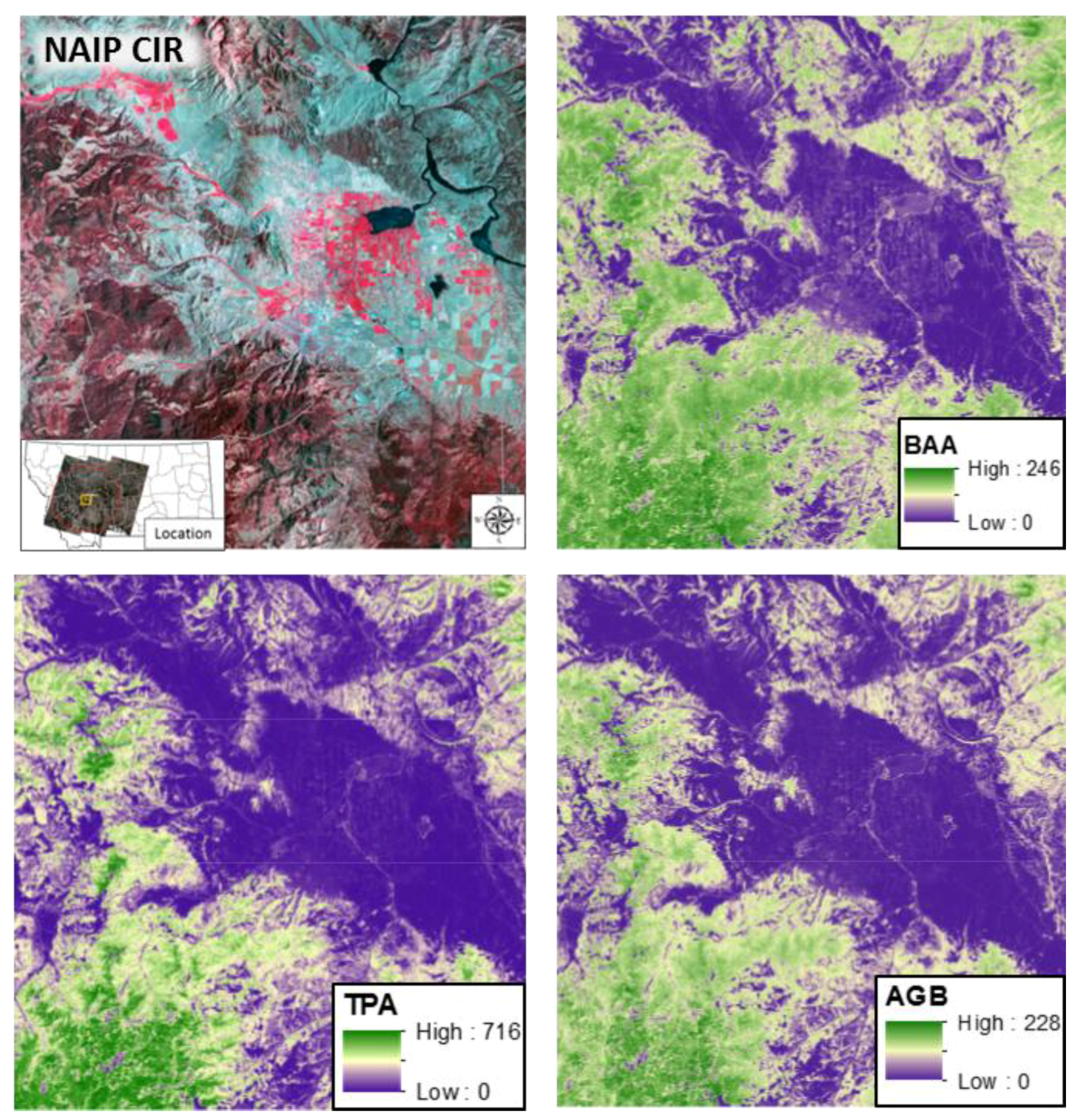
2.2. Biomass Stocks
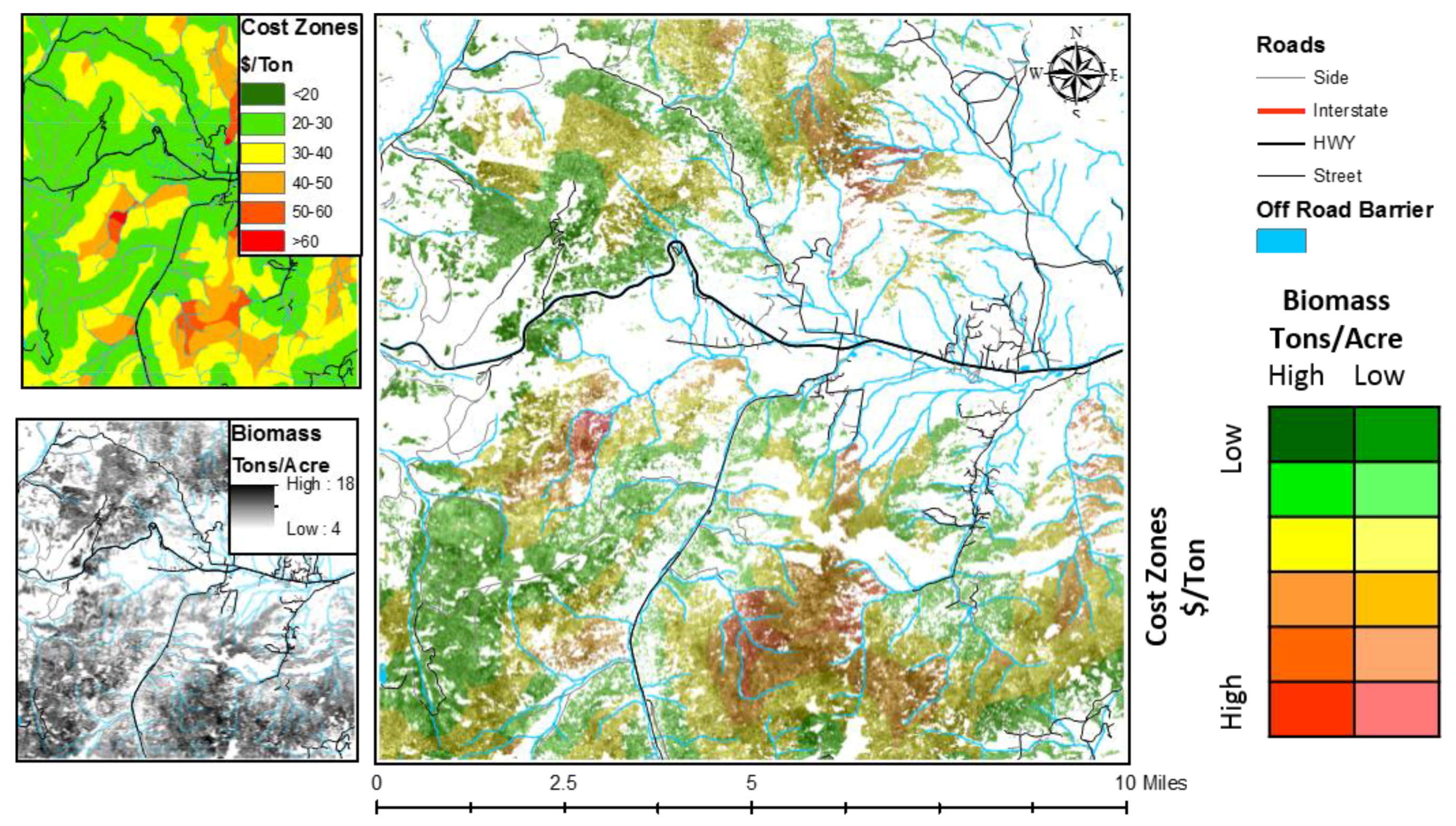
2.3. Biomass Costs
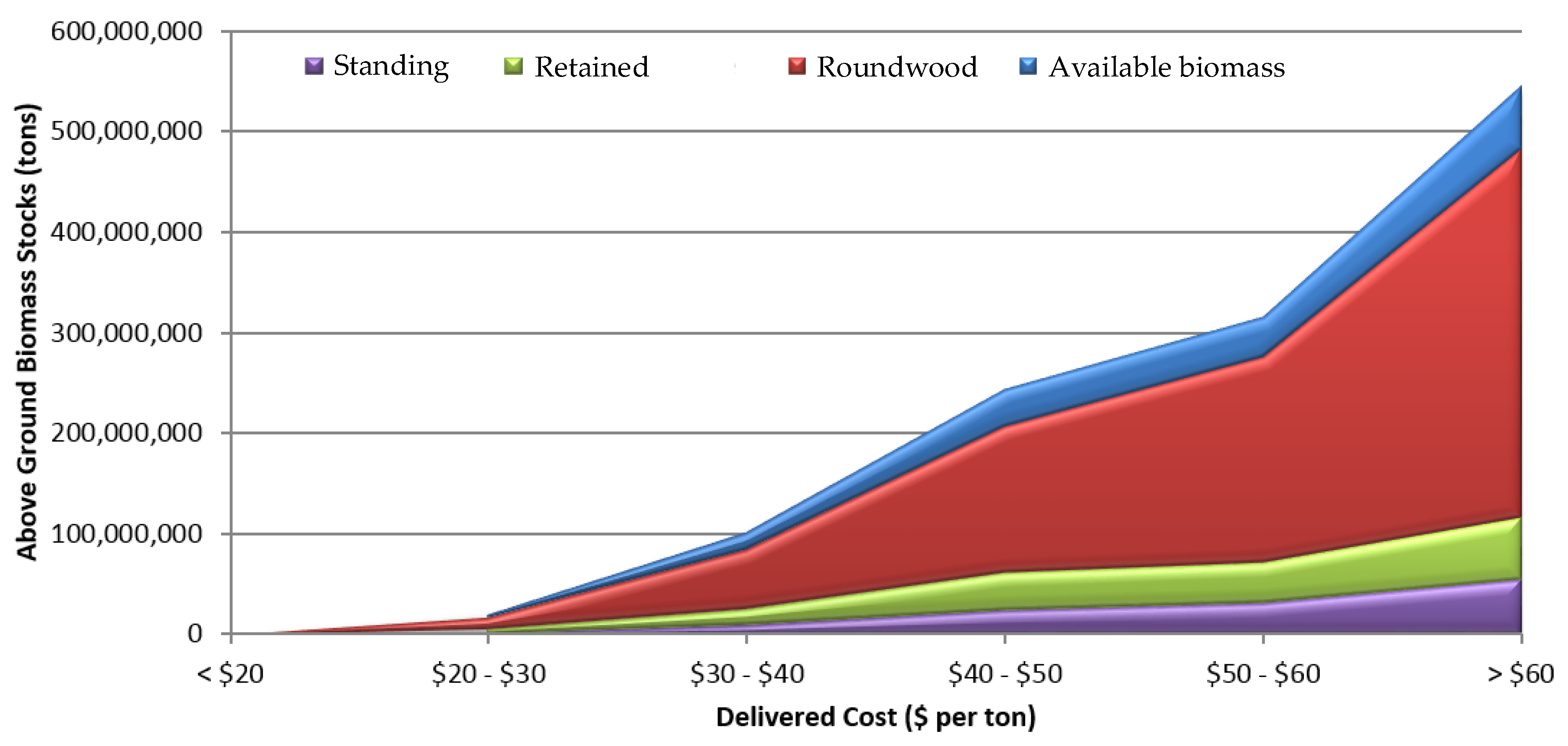
2.4. Woody Biomass Supply
2.5. Replicating This Approach
3. Results
3.1. Biomass Estimation
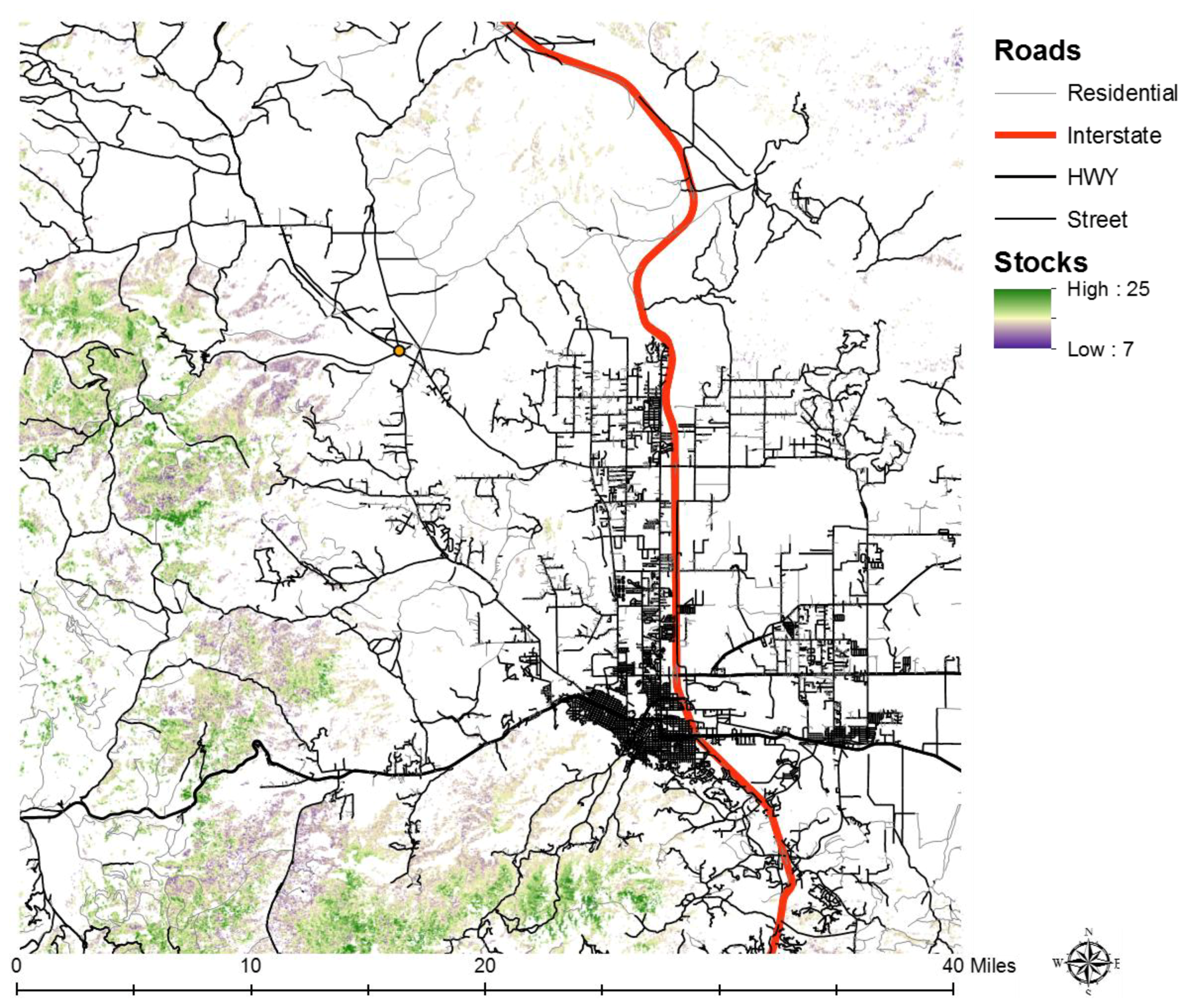
3.2. Delivered Costs
3.3. The Supply Chain
4. Discussion
5. Conclusions
Acknowledgments
Author Contributions
Conflicts of Interest
References
- Campbell, R.; Anderson, N.; Daugaard, D.; Naughton, H. Technoeconomic and policy drivers of project performance for bioenergy alternatives using biomass from beetle-killed trees. Energies 2018, 11, 293. [Google Scholar] [CrossRef]
- Keefe, R.; Anderson, N.; Hogland, J.; Muhlenfeld, K. Chapter 14: Woody biomass logistics. In Cellulosic Energy Cropping Systems; Karlen, D., Ed.; John Wiley and Sons: West Sussex, UK, 2014; pp. 251–279. [Google Scholar]
- Anderson, N.; Mitchell, D. Forest operations and woody biomass logistics to improve efficiency, value, and sustainability. Bioenergy Res. 2016, 9, 518–533. [Google Scholar] [CrossRef]
- Yue, D.; You, F.; Snyder, S. Biomass-to-bioenergy and biofuel supply chain optimization: Overview, key issues and challenges. Comput. Chem. Eng. 2014, 66, 36–56. [Google Scholar] [CrossRef]
- De Meyer, A.; Cattrysse, D.; Rasinmäki, J.; Van Orshoven, J. Methods to optimise the design and management of biomass-for-bioenergy supply chains: A review. Renew. Sustain. Energy Rev. 2014, 31, 657–670. [Google Scholar] [CrossRef]
- Zhang, F.; Johnson, D.; Sutherland, J. A GIS-based method for identifying the optimal location for a facility to convert forest biomass to biofuel. Biomass Bioenergy 2011, 35, 3951–3961. [Google Scholar] [CrossRef]
- Wells, L.; Chung, W.; Anderson, N.; Hogland, J. Spatial and temporal quantification of forest residue volumes and delivered costs. Can. J. For. Res. 2016, 46, 832–843. [Google Scholar] [CrossRef]
- Liu, Z.; Wang, S.; Ouyang, Y. Reliable biomass supply chain design under feedstock seasonality and probablistic facility disruptions. Energies 2017, 10, 1895. [Google Scholar] [CrossRef]
- Wu, J.; Wang, J.; McNeel, J. Economic modeling of woody biomass utilization for bioenergy and its application in central Applachia, USA. Can. J. For. Res. 2011, 41, 165–179. [Google Scholar] [CrossRef]
- Martinkus, N.; Latta, G.; Morgan, T.; Wolcott, M. A comparison of methodologies for estimating delivered forest residue volume and cost to a wood-based biorefinery. Biomass Bioenergy 2017, 106, 83–94. [Google Scholar] [CrossRef]
- Moller, B.; Nielsen, P. Analysing transport costs of Danish forest wood chip resources by means of continuous cost surface. Biomass Bioenergy 2007, 31, 291–298. [Google Scholar] [CrossRef]
- Hogland, J.; Anderson, N. Function modeling improves the efficiency of spatial modeling using big data from remote sensing. Big Data Cogn. Comput. 2017, 1, 3. [Google Scholar] [CrossRef]
- Perpiña, C.; Alfonso, D.; Pérez-Navarro, A.; Peñalvo, E.; Vargas, C.; Cárdenas, R. Methodology based on Geographic Information Systems for biomass logistics and transport optimization. Renew. Energy 2009, 34, 555–565. [Google Scholar] [CrossRef]
- Wells, L.A. Spatial Distribution and Quantification of Forest Treatment Residues for Bioenergy Production. Master’s Thesis, College of Forestry and Conservation, University of Montana, Missoula, MT, USA, 2013. Available online: https://scholarworks.umt.edu/etd/4177/ (accessed on 29 March 2018).
- Avery, T.; Burkhart, H. Forest Measurements, 4th ed.; McGraw Hill: Boston, MA, USA, 1994; p. 408. [Google Scholar]
- Rao, J.; Molina, I. Small Area Estimation: Second Edition; John Wiley & Sons: Hoboken, NJ, USA, 2015; p. 441. [Google Scholar]
- Hogland, J.; Anderson, N.; Chung, W.; Wells, L. Estimating forest characteristics using NAIP imagery and ArcObjects. In Proceedings of the 2014 ESRI Users Conference, San Diego, CA, USA, 14–18 July 2014. [Google Scholar]
- Bioenergy Alliance Network of the Rockies (BANR). Available online: http://banr.nrel.colostate.edu/ (accessed on 14 January 2018).
- USCB. American Fact Finder. Available online: http://factfinder2.census.gov/faces/nav/jsf/pages/index.xhtml (accessed on 25 March 2014).
- State of Montana. Montana is Bioenergy Country: Developing Biomass Fuels for Tomorrow’s Energy. Available online: http://commerce.mt.gov/content/Energy/docs/EnergyBrochures/BioenergyBrochure.pdf (accessed on 25 March 2014).
- Hunter, L. Renewable Energy in the 50 States: Western Region; American Council on Renewable Energy (ACORE): Washington, DC, USA, 2013; p. 40. Available online: http://www.acore.org/images/documents/Western_Region_Report.pdf (accessed on 25 March 2014).
- Department of Commerce. Montana Department of Commerce—Energy Promotion and Development Bureau. Available online: http://commerce.mt.gov/energy/default.mcpx (accessed on 25 March 2014).
- HB25. Electric Utility Industry Generation Reintegration Act. Available online: http://leg.mt.gov/css/Committees/interim/2007_2008/energy_telecom/assigned_studies/hb25page/hb25.asp (accessed on 25 March 2014).
- HB3. Jobs and Energy Development Incentives Act. Available online: http://leg.mt.gov/bills/specsess/0507/billpdf/HB0003.pdf (accessed on 25 March 2014).
- Lewis & Clark County. Lewis and Clark County Brownfields Project. Available online: http://www.lcc-brownfields.com/ (accessed on 25 March 2014).
- Kim, Y.; Chung, W.; Han, H.; Anderson, N. Effect of downed trees on harvesting productivity and costs in beetle-killed stands. For. Sci. 2017, 63, 596–605. [Google Scholar]
- USFS. Collaborative Forest Landscape Restoration Program Overview. Available online: http://www.fs.fed.us/restoration/CFLRP/overview.shtml (accessed on 25 March 2014).
- USFS. Western Bark Beetle Strategy. Available online: http://www.fs.fed.us/publications/bark-beetle/bark-beetle-strategy-appendices.pdf (accessed on 25 March 2014).
- City of Helena. Ten Mile Watershed Projects. Available online: http://www.helenamt.gov/tmwp.html (accessed on 14 January 2018).
- Thompson, M.; Anderson, N. Modeling fuel treatment impacts on fire suppression cost savings: A review. Calif. Agric. 2015, 69, 164–170. [Google Scholar] [CrossRef]
- USCB. TIGER/Line Shapefiles [Machine-Readable Data Files]. Available online: https://www2.census.gov/geo/tiger/TGRGDB13/ (accessed on 18 April 2018).
- Gesch, D.; Oimoen, M.; Geenlee, S.; Nelson, C.; Steuck, M.; Tyler, D. The National Elevation Dataset. Photogramm. Eng. Remote Sens. 2002, 68, 5–11. [Google Scholar]
- NHD. National Hydrography Dataset. Available online: http://datagateway.nrcs.usda.gov (accessed on 6 February 2018).
- U.S. Department of Agriculture Forest Service (USFS). Forest Inventory and Analysis National Core Field Guide: Field Data Collection Procedures for Phase 2 Plots, 2012 Version 6.0. Vol. 1. Internal Report. Available online: http://www.fia.fs.fed.us/library/field-guides-methodsproc/docs/2013/Core%20FIA%20P2%20field%20guide_6-0_6_27_2013.pdf (accessed on 6 May 2014).
- National Agriculture Imagery Program (NAIP). National Agriculture Imagery Program (NAIP) Information Sheet. 2012. Available online: http://www.fsa.usda.gov/Internet/FSA_File/naip_info_sheet_2013.pdf (accessed on 14 May 2014).
- Hogland, J.; Anderson, N. Estimating FIA plot characteristics using NAIP imagery, function modeling, and the RMRS Raster Utility coding library. In Pushing Boundaries: New Directions in Inventory Techniques and Applications, Proceedings of the Forest Inventory and Analysis (FIA) Symposium, Portland, OR, USA, 8–10 December 2015; General Technical Report PNW-GTR-931; Stanton, S.M., Christensen, G.A., Eds.; U.S. Department of Agriculture, Forest Service, Pacific Northwest Research Station: Portland, OR, USA; pp. 340–344.
- Jenkins, J.; Chojnacky, D.; Heath, L.; Birdsey, R. National-scale biomass estimation for United States tree species. For. Sci. 2003, 49, 12–35. [Google Scholar]
- U.S. Forest Service. Red Mountain Flume Chessman Reservoir Project. Available online: https://data.ecosystem-management.org/nepaweb/nepa_project_exp.php?project=41571 (accessed on 14 January 2018).
- RMRS. RMRS Raster Utility. 2014. Available online: http://www.fs.fed.us/rm/raster-utility (accessed on 3 March 2018).
- ESRI. Cost Path. Available online: http://desktop.arcgis.com/en/arcmap/10.3/tools/spatial-analyst-toolbox/cost-path.htm (accessed on 6 February 2018).
- Lauer, C.; McCaulou, J.; Sessions, J.; Capalbo, S. Biomass supply curves for western juniper in Central Oregon, USA, under alternative business models and policy assumptions. For. Policy Econ. 2015, 59, 75–82. [Google Scholar] [CrossRef]
- Smith, B.; Miles, P.; Perry, C.; Pugh, S. Forest Resources of the United States, 2007; General Technical Report WO-78; Washington Office, Forest Service, U.S. Department of Agriculture: Washington, DC, USA; p. 336.


| Treatment | Criteria | Threshold |
|---|---|---|
| Stand replacement | Basal area | >100 ft2/ac (>23 m2/ha) |
| Stand density | 200 to 400 trees/ac (46 to 92 trees/ha) | |
| Thinning | Basal area | >100 ft2/ac (>23 m2/ha) |
| Stand density | >400 trees/ac (>92 trees/ha) |
| Treatment | Description | % AGB Cut Assumption |
|---|---|---|
| Stand replacement | Trees are cut to mimic a stand replacement event; most trees are cut | 90% of AGB is cut, 10% of AGB is not cut and remains in the standing pool |
| Thinning | Trees are cut to reduce the basal area and QMD to a specific target | % AGB cut to move pre-treatment BAA to target BAA; 60 ft2 per acre (14 m2 per ha), which is left in the standing pool |
| Component | Type | Value | Units |
|---|---|---|---|
| On-road | Machine Rate | 90 | $/hour |
| Speed | 15–65 (24–105) | mi/h (km/h) | |
| Payload | 28 (25.4) | tons (tonnes) | |
| Off-road | Machine Rate | 85 | $/hour |
| Speed | 3.6 (5.8) | mi/h (km/h) | |
| Payload | 4.0 (3.6) | tons (tonnes) | |
| Operations | Harvesting | 15 (13.6) | $/ton ($/tonne) |
| Other | Administrative | 0 (0) | $/ton ($/tonne) |
| Query | Speed mi/hr (km/hr) |
|---|---|
| MTFCC = “S1400”: Local Road, Rural Road, City Street | 30 (48) |
| MTFCC = “S1200”: Secondary road | 50 (80) |
| MTFCC = “S1100”: Primary road | 60 (97) |
| NOT (MTFCC = “S1400” OR MTFCC = “S1200” OR MTFCC = “S1100”) | 20 (32) |
© 2018 by the authors. Licensee MDPI, Basel, Switzerland. This article is an open access article distributed under the terms and conditions of the Creative Commons Attribution (CC BY) license (http://creativecommons.org/licenses/by/4.0/).
Share and Cite
Hogland, J.; Anderson, N.; Chung, W. New Geospatial Approaches for Efficiently Mapping Forest Biomass Logistics at High Resolution over Large Areas. ISPRS Int. J. Geo-Inf. 2018, 7, 156. https://0-doi-org.brum.beds.ac.uk/10.3390/ijgi7040156
Hogland J, Anderson N, Chung W. New Geospatial Approaches for Efficiently Mapping Forest Biomass Logistics at High Resolution over Large Areas. ISPRS International Journal of Geo-Information. 2018; 7(4):156. https://0-doi-org.brum.beds.ac.uk/10.3390/ijgi7040156
Chicago/Turabian StyleHogland, John, Nathaniel Anderson, and Woodam Chung. 2018. "New Geospatial Approaches for Efficiently Mapping Forest Biomass Logistics at High Resolution over Large Areas" ISPRS International Journal of Geo-Information 7, no. 4: 156. https://0-doi-org.brum.beds.ac.uk/10.3390/ijgi7040156