Article

Shaking Maps Based on Cumulative Absolute Velocity and Arias Intensity: The Cases of the Two Strongest Earthquakes of the 2016–2017 Central Italy Seismic Sequence

Osservatorio Nazionale Terremoti, Istituto Nazionale di Geofisica e Vulcanologia, Rende 87036, Italy
ISPRS Int. J. Geo-Inf. 2018, 7(7), 244; https://0-doi-org.brum.beds.ac.uk/10.3390/ijgi7070244
Submission received: 29 March 2018 / Revised: 4 June 2018 / Accepted: 13 June 2018 / Published: 22 June 2018
(This article belongs to the Special Issue Natural Hazards and Geospatial Information)

Abstract

:
By referring to the two strongest earthquakes of the 2016–2017 Central Italy seismic sequence, this paper presents a procedure to make shaking maps through empirical relationships between macroseismic intensity and ground-motion parameters. Hundreds of waveforms were processed to obtain instrumental ground-motion features which could be correlated with the potential damage intensities. To take into account peak value, frequency, duration, and energy content, which all contribute to damage, cumulative absolute velocity and Arias intensity were used to quantify the features of the ground motion. Once these parameters had been calculated at the recording sites, they were interpolated through geostatistical techniques on the whole struck area. Finally, empirical relationships were used for mapping intensities, i.e., potential effects on the built environment. The results referred to both earthquake scenarios that were analyzed and were also used for assessing the influence of the spatial coverage of the instrumental network. In fact, after the first events, the Italian seismic network was subjected to the addition and thickening of sensors in the epicentral area, especially. The results obtained by models only dependent on ground-motion parameters or even on the epicentral distance were compared with the official ShakeMaps and the observed intensities for assessing their reliability. Finally, some suggestions are proposed to improve the procedure that could be used for rapidly assessing ground shaking and mapping damage potential producing useful information for non-expert audience.

1. Introduction

Observations about the effects of seismic shakings are at the base of macroseismic intensity scales, such as Rossi–Forel (RF, [1]), Mercalli–Cancani–Sieberg (MCS, Sieberg, [2]), Modified Mercalli (MM, [3,4]), Medvedev–Sponheuer–Kárník (MSK, [5]), and the European Macroseimic Scale (EMS, [6]). Instrumental measures, conversely, can be used for quantitative assessments of the ground motion based on real recordings. A topic of great interest for earthquake engineering is the assessment of the damage potential due to an earthquake based on the distribution of the felt intensity. This relation depends on some variable elements such as local geological conditions, the type of buildings and their construction period, uncertainty related to materials, and the condition of the constructions before earthquake. However, today, instrumental seismology offers the possibility of correlating many observed data (macroseismic intensity) with parameters widely used for engineering purposes (ground-motion measures), thus making it possible to obtain empirical models for linking the two variables. On the other hand, in many areas of the world strongly exposed to seismic hazard, seismic networks can provide ground-motion recordings with dense spatial coverage, and these data are often available in a relatively short period of time. Therefore, these data can be used to determine the location and magnitude of the earthquake, as well as ground-motion shaking maps by interpolation of ground-motion parameters, which are directly obtained by recordings. In addition, based on the ground-motion shaking maps, it is possible to produce intensity maps, which have become adopted worldwide to provide quantitative, first-order assessments of the level of shaking and of the extent of potential earthquake damage. Intensities have been found informative by non-expert audiences unfamiliar with instrumental ground-motion parameters [7,8]. In addition, intensities predicted on a regular grid can be useful to make inferences about the level of strong ground motion experienced after a larger earthquake in localities where little instrumental data are available [9].
Some attempts have been made to correlate macroseismic intensity with the peak or spectral features, most frequently to peak ground acceleration (PGA), since this parameter is related to seismic-resistant design, to peak ground velocity (PGV) or to PseudoSpectral Acceleration (PSA) (e.g., [10,11,12,13,14,15,16,17,18,19]).
According to the method proposed by Wald et al. [7,20,21], in Italy, ground-motion shaking maps in terms of PGA, PGV, and PSA at 0.3, 1.0, and 2.0 s are elaborated by National Institute of Geophysics and Volcanology; hence, intensity ShakeMaps are obtained through conversion relationships between peak ground-motion parameters and the MCS intensities [8,9].
To take into account other ground-motion characteristics, such as frequency, duration, and energy content, which all contribute to structural damage, empirical equations have been proposed to correlate cumulative parameters that are more efficient for representing earthquake destructiveness potential against the felt intensity. Two of the simplest and most studied parameters are Arias intensity (AI, [22]) and cumulative absolute velocity (CAV, [23]), mathematically defined by Equations (1) and (2), respectively:
A I = π 2 g 0 t m a x a ( t ) 2 d t
C A V = 0 t m a x | a ( t ) | d t
where a(t) is the value of acceleration at time t and tmax is the total duration of the ground motion.
Moreover, the standardized cumulative absolute velocity (CAVSTD) is used to prevent low-amplitude, non-damaging ground motion from contributing to the CAV. In fact, CAVSTD is mathematically defined by Equation (3) [24]:
C A V S T D = i = 1 N [ H ( P G A i a t h r ) i 1 i | a ( t ) | d t ]
where N is the number of non-overlapping one-second time intervals, PGAi is the peak ground acceleration in the time interval i, athr is the threshold value of acceleration, and H(x) is the Heaviside step function given by Equation (4):
H ( x ) = { 0 ,     x < 0 1 ,     x 0
If the value of acceleration in the time interval i is greater than athr, the whole interval of the record contributes to the CAVSTD. Therefore, CAVSTD will always be equal to or less than CAV; in fact, the difference can be quite large for long-duration and small-amplitude records [25].
Both AI and CAV (or CAVSTD) include the cumulative effects of the ground-motion duration differently based on the peak ground motion and response spectral parameters commonly used in engineering analysis. However, these parameters also have some limitations, i.e., neither AI nor CAV explicitly account for arrival time of the different phases of energy [25] such as a large velocity pulse, which can affect the structural response due to near-source ground motion (e.g., [26]).
Cabanas et al. [27] tested several relationships between representative parameters of ground-motion energy and damage data using 25 recordings from four earthquakes in Italy (ML between 4.7 and 6.5). They observed that AI and standardized CAVSTD showed good correlation with macroseismic effects observed after an earthquake. They further correlated AI and different versions of CAVSTD characterized by values of threshold acceleration from 5 to 25 cm/s2 with MSK intensity and observed damage. They concluded that these parameters showed good correlation only with observed structural damage for the poorest construction type (i.e., buildings in field stone, rural structures, adobe houses, and clay houses).
Koliopulos et al. [28] conducted work on a Greek strong motion database in order to obtain regression equations for MM intensity and various ground-motion parameters, such as duration, CAV, AI, and Housner spectrum intensity. About 10 years later, Tselentis and Danciu [29] also developed relationships for PGA, PGV, AI, and CAV, correlated with the observed MM intensity for a Greek strong motion database of 310 records from 89 earthquakes (MW up to 6.9). In order to reduce the observed biases in the residuals, they found that the magnitude, distance, and site conditions should be introduced as variables in the relationships. Their final relationships showed standard deviations between 0.649 and 0.679, indicating that all four physical parameters were equally good at predicting MM intensities.
As found by analyzing different studies in the literature, Campbell and Bozorgnia [25] assert that some version of CAV is superior to (or as good as) peak-amplitude, spectral-response, duration-based, and damage-related intensity based on their correlation with seismic intensity or observed damage and their high level of predictability (i.e., their relatively small standard deviations).
In this framework, the paper mainly focuses on testing a procedure that is able to produce reliable shaking maps obtained by CAV and AI ground-motion parameters against macroseismic intensity. The presented procedure is applied to the instrumental data available for the main earthquakes of the 2016–2017 Central Italy seismic sequence, i.e., MW 6.0 Amatrice and MW 6.5 Norcia earthquake. The study area and data from recordings of the ground motion are presented initially (Section 2.1). The methodology is explicated in order to understand the data processing both for interpolating engineering parameters with geostatistical techniques (Section 2.2) and for correlating these features with the macroseismic intensity (Section 2.3). The application to the two earthquakes of the Central Italy seismic sequence is shown, and a comparison with the official ShakeMaps is proposed (Section 3). Finally, conclusions and any potential improvements are highlighted (Section 4).

2. Materials and Methods

In the first subparagraph, the data and study area are presented, which is followed by the procedure. Details are provided about the two phases: (1) the interpolation of the engineering ground-motion parameters CAV and AI through geostatistical techniques and (2) the application of relationships between these parameters and macroseismic intensity.

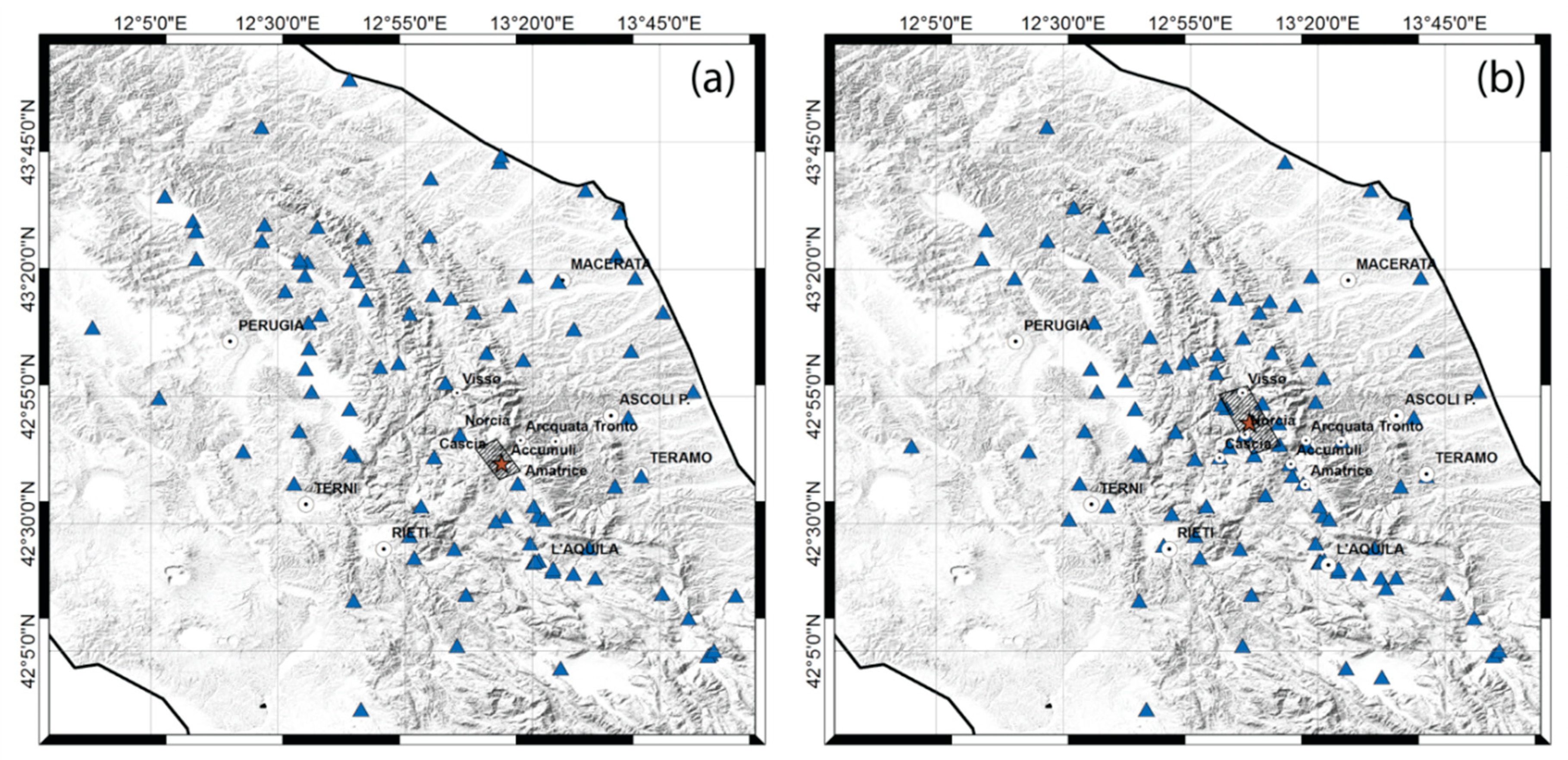
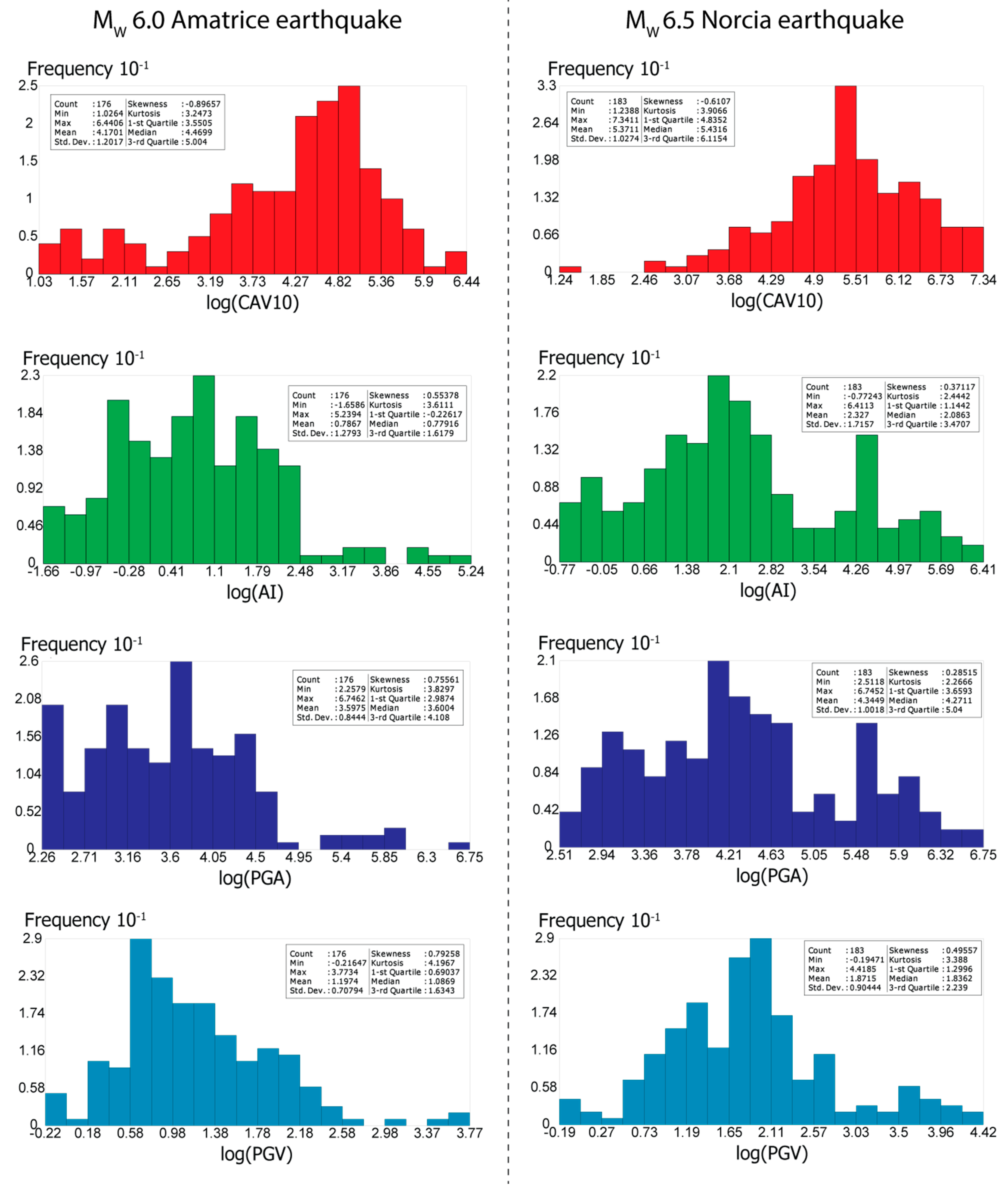
2.1. Study Area and Data

On 24 August 2016, a MW 6.0 (at 01:36:32 UTC) earthquake struck an extended region of the Central Apennine, which is one of the most seismically active areas in Italy. This strong earthquake (see red star in Figure 1a) occurred close to the Accumuli village (epicentral distance about 1 km) and the Amatrice towns (epicentral distance 10 km), producing some casualties and strong damage to the buildings (e.g., [30,31]) and historic heritage (e.g., [32]) in many towns around the epicenter. The following seismic sequence produced hundreds of aftershocks per day [33], including a MW 5.4 earthquake on August 24 (at 02:33:34 UTC). About two months after the Amatrice earthquake, on 26 October, two other moderate–strong earthquakes (MW 5.4 and 5.9) occurred at about 14 km NNE of Norcia, near the Visso village. All of these earthquakes, preceding the strongest event, a MW 6.5 on 30 October (at 06:40:18 UTC), occurred at about 5 km north of Norcia (see red star in Figure 1b). This terrible seismic sequence had widespread effects on the built environment—several historic centers were significantly damaged and/or partially destroyed. In addition, the strong events triggered ground failures and deep-seated landslides (e.g., [34,35]). In this framework, the Amatrice earthquake caused about 300 casualties due to the collapse of several buildings, but luckily, the following ones did not produce victims mainly because immediately after the first event, people had been evacuated.
In this work, data referring to the MW 6.0 Amatrice earthquake (see Figure 1a) and the MW 6.5 Norcia earthquake (see Figure 1b) have been analyzed. The two earthquakes were mainly recorded through the Italian national accelerometric network, operated by the Department of Civil Protection. The recordings are available on the Italian Accelerometric Archive Itaca [36]. Figure 1 maps the two configurations of the seismic network for the two earthquakes; to be noted is the different concentration of seismic stations close to the epicenters during the earthquake of Norcia (Figure 1b) with respect to that of Amatrice (Figure 1a).
The horizontal acceleration time histories, with two orthogonal components for each site, were processed for calculating CAVSTD with a threshold acceleration of 10 cm/s2, AI, PGA, and PGV.
For the rest of the paper, for simplicity, CAV10 indicates the standardized cumulative absolute velocity with a threshold acceleration of 10 cm/s2.
It should be noted that no site corrections were applied to the parameters to avoid introducing further uncertainties. In fact, for the recording sites, the soil classification was available linked to the near-surface velocities, i.e., the average of shear-wave velocities from the surface to 30-m depth (Vs30); however, this parameter seemed to suffer from low accuracy and poor correlation (e.g., [37,38]). Since it was decided not to introduce site correction in the processing, the recordings on site classified as D (Vs30 < 180m/s) or E (alluvium layer with thickness between 5 m and 20 m, and Vs30 < 360 m/s) following Eurocode 8 were excluded, i.e., eight recording sites for both earthquakes; in fact, these sites are considered potentially subject to the more significant local effects.
The distributions of the ground-motion parameters for the two earthquakes are shown in Figure 2 after the logarithmic transformation.

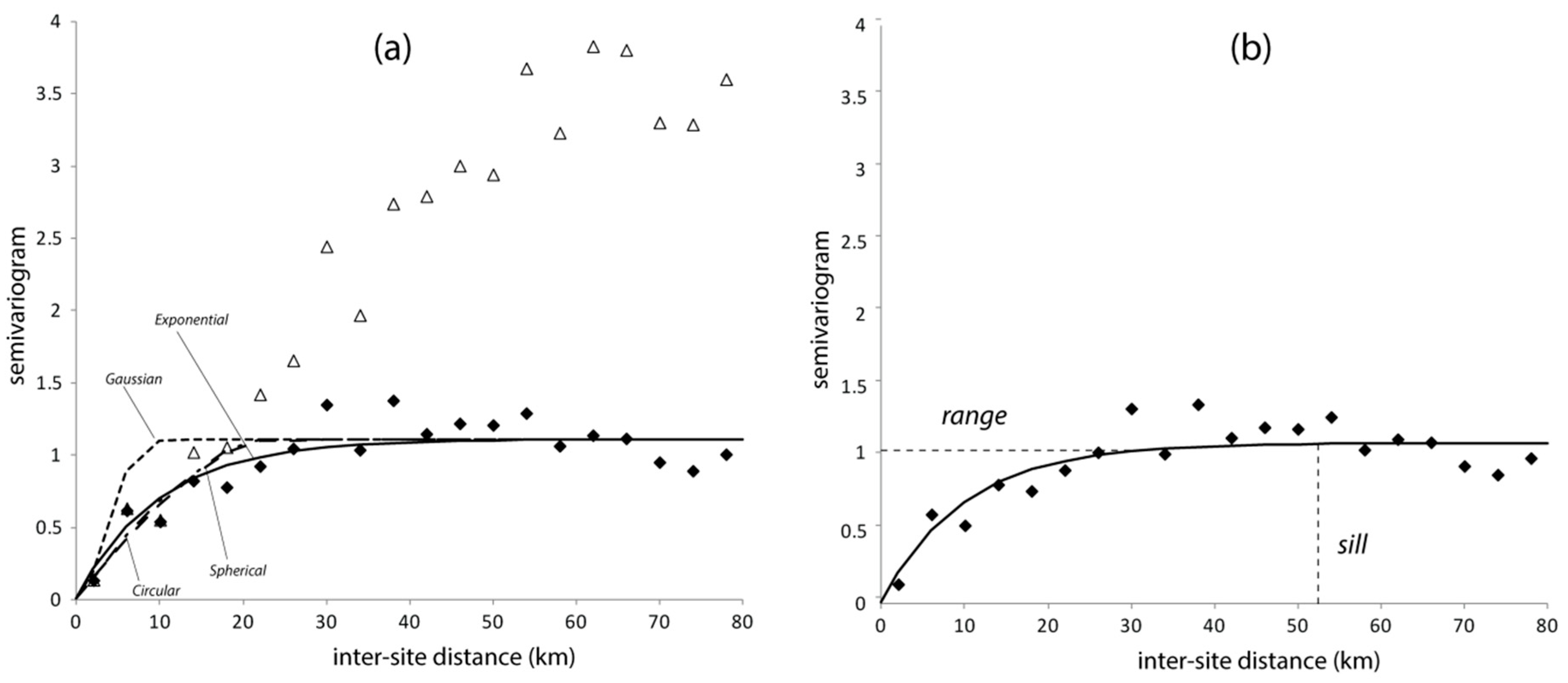
2.2. Geospatial Interpolation
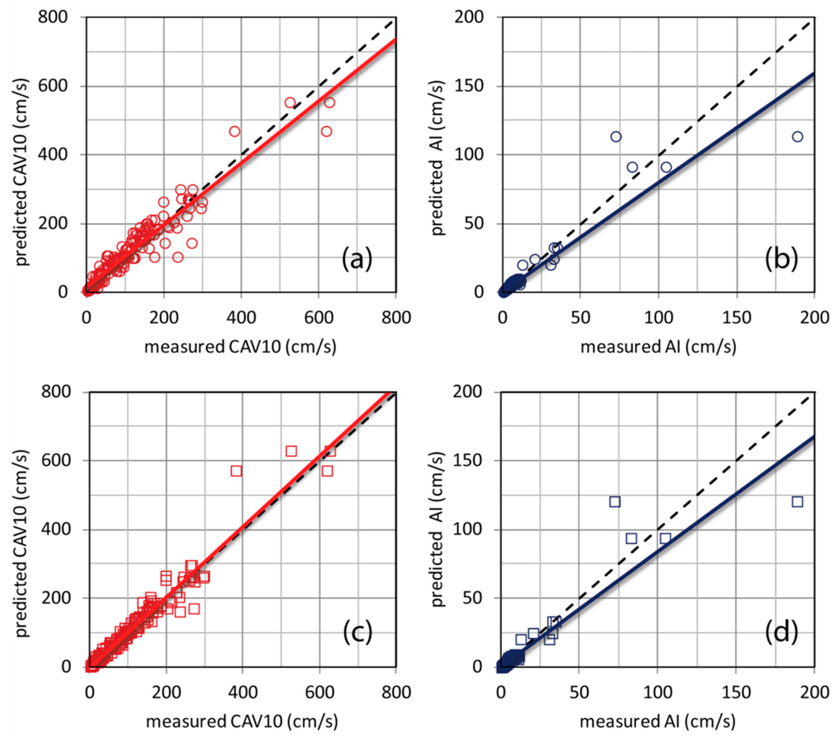
Interpolations were performed through kriging techniques that apply linear-weighted averaging methods with weights dependent not only on the distance, but also on the direction of the neighboring data to the unsampled location. In addition, for both analyzed cases, the cokriging method was applied using alternatively CAV10 and AI, with one as primary data and the other as secondary data besides PGA and PGV. The latter method considers the correlations among the different parameters.
The ground motion features obtained from the horizontal components (north-south and east-west) were used in the interpolation process, therefore two values were related to each recording site. Extensive discussion of the theoretical basis of geostatistics applied to the environmental process can be found in the literature (e.g., [39,40,41,42]). The spatial dependence between neighboring observations is often expressed through the semivariogram, which is a widely used geostatistical tool for modelling regionalized variables such as spatially distributed ground-motion measures [43,44,45,46]. Under the hypothesis of second-order stationarity and isotropy, the empirical semivariogram, γ(h), can be defined as half the average squared difference between all points located at distance h, and it is mathematically expressed by Equation (5):
γ ( h ) = 1 2 N ( h ) i = 1 N ( h ) [ Z ( x i ) Z ( x i + h ) ] 2
where Z(x) indicates the magnitude of the variable at location x, Z(x + h) that at distance h from the previous one, and N(h) is the total number of pairs of data that are separated by a distance h.
However, it is not always the case that two sites are separated by exact lag; therefore, a distance bin [h − ∆h, h + ∆h] is defined. In this work, a lag size between 4 and 5 km was used to group data pairs for computing semivariograms in order to ensure at least some pairs of data in each bin and to compensate for the poor data within the short separation distance.
Practically, the presence of a trend is detected when the semivariogram does not have a stable sill, i.e., the maximum value of the semivariogram (cf. Figure 3a,b). For this reason, before proceeding to calculate semivariograms, variables were corrected through detrending processing. In this work, this was done by fitting a trend surface to the original values by weighted least squares and then subtracting the value of the trend surface function from the original ones, thus constructing a new residuals variable. First-order polynomials were used for removing overall trend and bias.
A mathematical model must be used to compute the semivariogram value for any possible sampling interval. Practically, the coefficients are estimated so that the chosen model best fits semivariogram values that are calculated for defined lag distances. Most commonly used models are circular, spherical, exponential, and Gaussian [39,40], which are described in Equations (6)–(9) (cf. Figure 3a).
Circular semivariogram model:
{ γ ( h ) = 2 s π [ h R 1 ( h R ) 2 + a r c s i n ( h R ) ] + n s           for           R < h     for   0 h R
Spherical semivariogram model:
{ γ ( h ) = s   [ 3 2 h R 1 2 ( h R ) 3 ] + n s             for           R < h     for   0 h R
Exponential semivariogram model:
  γ ( h ) = s [ 1 e x p ( 3 h R ) ] + n    
Gaussian semivariogram model:
  γ ( h ) = s   [ 1 e x p ( 3 ( h R ) 2 ) ] + n    
In the previous equations: n is the nugget, i.e., the value of the empirical semivariogram corresponding to zero intersite distance; s is the sill, i.e., the maximum value of the semivariogram (cf. Figure 3b); and R is the range, which represents the intersite distance at which the difference between the semivariogram and the sill becomes negligible (cf. Figure 3b). In this work, the weighted least squares method was then used as a reference to manually adjust parameters for well-fitting semivariograms at short interdistance.
The reliability of the semivariogram model can be tested through the cross-validation technique, which is able to exclude one datum at a time from the dataset and, hence, to estimate this value through remaining those using the different semivariogram models. The interpolated values are compared with the actual ones and the model producing most accurate predictions is kept [39,42]. By means of cross-plotting between estimated and true values, the validation can be performed and the correlation coefficient calculated.
Kriging provides the solution to the problem based on a continuous model of the stochastic spatial variation. It takes into account property variation in space through the semivariogram model. Since the original formulation, different kinds of kriging techniques have been elaborated based on linear or nonlinear methods to deal with increasingly complex problems. The ordinary kriging technique is the most robust interpolation estimator used to find the best linear unbiased estimate. The estimates are the weighted linear combination of the data, where the weights are assigned to the sample data within the neighborhood of the point to be estimated in such a way as to minimize the estimation of variance [40].
The general equation of the kriging estimator is
Z * ( x 0 ) = i = 1 n λ i Z ( x i )
where Z*(x0) is the estimated value at point x0, Z(xi) is the known value at point xi, and λi is the weight associated with the data. In order to achieve unbiased estimations, the following set of equations should be solved simultaneously:
{ i = 1 n λ i γ ( x i ,   x j ) μ = γ ( x i ,   x j ) i = 1 n λ i = 1                                                                          
where μ is the Lagrange multiplier and γ(xi, xj) is the value of the semivariogram between the data points xi and xj.
The cokriging method takes into account information on several variable types. In fact, the primary data are estimated by the secondary ones. For this method, Equation (11) can be rewritten as follows:
{ l = 1 v i = 1 n l λ i l γ l v ( x i ,   x j ) μ v = γ u v ( x j ,   x ) i = 1 n l λ i l = { 1 ,       1 = u 0 ,       1 u                                                                          
where u and v are the primary and secondary variables, respectively. The u and v are cross-correlated and the covariate contributes to the estimation of the primary value. Therefore, this method requires estimating the autocorrelation for each variable by mean of Equation (5) and the cross-correlation between the primary variable and each secondary one by Equation (13):
γ u v ( h ) = 1 2 N ( h ) i = 1 N ( h ) [ Z u ( x i ) Z u ( x i + h ) ] [ Z v ( x i ) Z v ( x i + h ) ]
Theoretically, cokriging can improve predictions obtained by kriging; in fact, if there is no cross-correlation, the method falls back on autocorrelation. However, each time the unknown autocorrelation parameters are calculated, it introduces more variability, so the gains in precision of prediction may not be worth the additional computational effort.

Accuracy Assessment

The predicted values obtained by different geostatistical methods were compared with the truth data to analyze their similarity. Three indexes were calculated for each model: normalized mean absolute error (NMAE), root mean squared error (RMSE), and the Pearson correlation coefficient (R2). To evaluate the indexes, Equations (14)–(16) were used:
N M A E = i = 1 n | t i p i | n i = 1 n t i n
  R S M E = i = 1 n ( t i p i ) 2 n
  R 2 = i = 1 n ( t i t ¯ ) ( p i p ¯ ) i = 1 n ( t i t ¯ ) 2 ( p i p ¯ ) 2
where ti and pi are truth and predicted values, respectively, of the examined parameter at the ith point, whereas t and p overmarked are the average values, and n is the number of the measurement points. Based on these indexes, the reliability was assigned to the models.

2.3. Relationships of Macroseismic Intensity with Ground-Motion Parameters

Three different predictive relationships were used for mapping the macroseismic intensity, which are those proposed by Cabanas et al. [27] (reported as CAB97 later), Koliopulos et al. [28] (KOL98), and Tselentis and Danciu [29] (T&D08). These predictive models were selected mainly for two reasons: (1) they are derived from data close to the study area and (2) the relationships based both on cumulative absolute velocity and Arias intensity were obtained. The relationships were based on the mean of the observed ground-motion parameters at each level of macroseismic intensity, and they were expressed by means of the following mathematical form:
I = a + b × log ( Y )
where I is the macroseismic intensity, a and b are the coefficients of the regression curves, and log (Y) is the natural logarithm for CAB97 and KOL98 or the base-10 logarithm for T&D08 of the ground-motion parameters (CAV10 or AI). It is worth pointing out that cumulative absolute velocity with the acceleration threshold of 20 cm/s2 was used in CAB97 and KOL98, whereas 10 cm/s2 was used in T&D08; however, in this work, CAV10 was always used to obtain precautionary values. The correlations between macroseismic intensity and ground-motion parameters were obtained considering the felt intensities within a circular area surrounding the recording station. According to the suggestion of Tselentis and Danciu [29], since the scatter associated with the mean values of their relationship is relatively large (within one to two units), the model dependent on the base-10 logarithm of the epicentral distance was also used, for which the scatter was reduced to within one-half and one unit. This latter model is hereinafter reported as T&D08-2. Please note that, although this latter model takes into account the local geological conditions by simply subtracting 0.105 from the MM intensity in the case of soft soils, as a precaution, this term was not considered in the following predictions.
To summarize, the regression models dependent only on ground-motion parameters (CAB97, KOL98, and T&D08) can be used as rapid damage assessment tools, regardless of the epicenter location. Alternatively, if the epicenter is known with good reliability, the predictive model T&D08-2 may also be used.

3. Results and Discussion

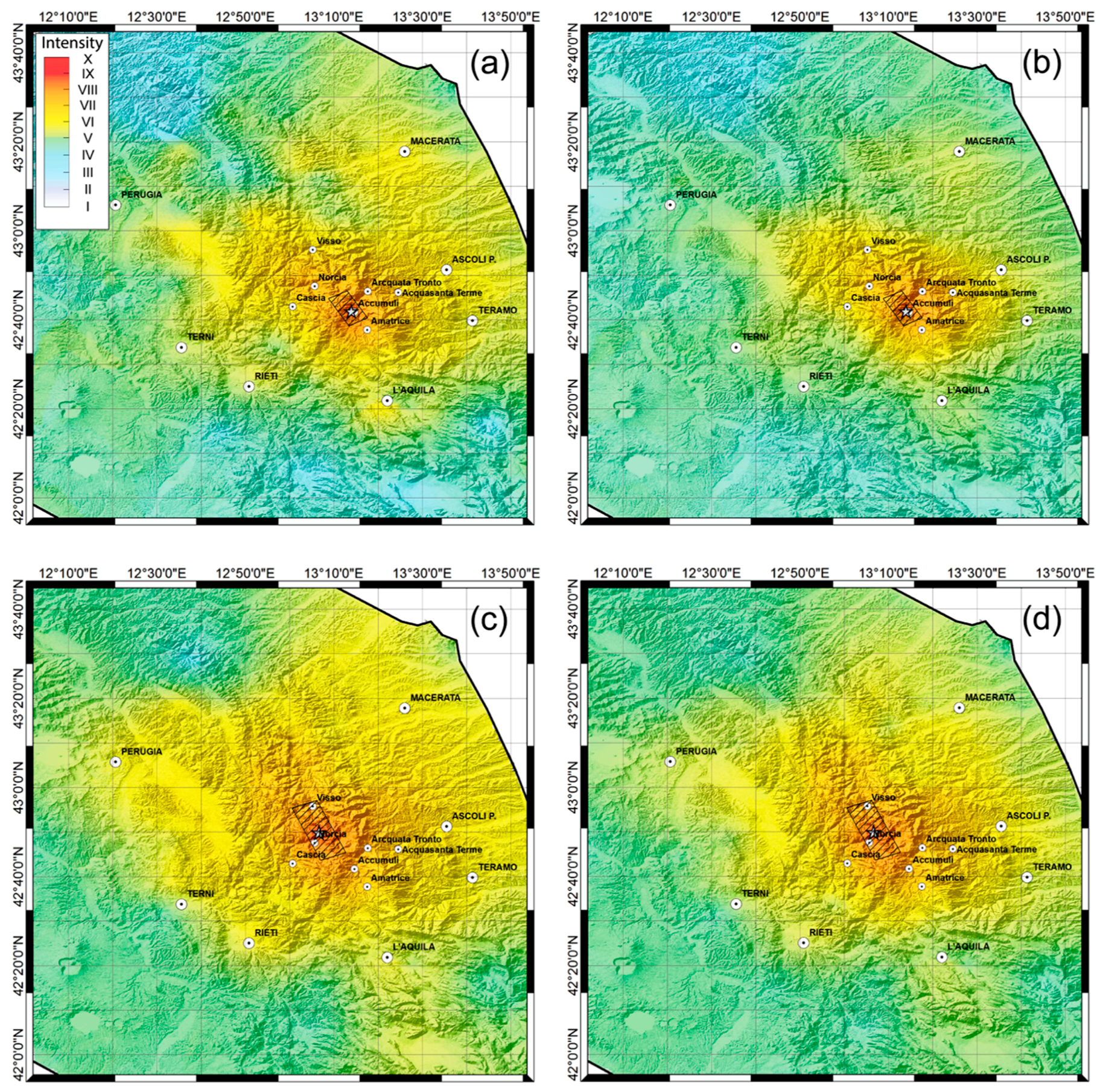
3.1. Interpolation of the Strong-Motion Parameters

To interpolate the CAV10 and AI ground-motion parameters, kriging and cokriging methods were used assuming different models to fit the variogram values: circular, spherical, exponential, Gaussian, and rationale quadratic. The cokriging method was applied assuming alternatively CAV10 and AI as primary and the other one with PGA and PGV as secondary variables.
The accuracy of prediction for the two methods and different models are reported in Table 1, for ground-motion parameters related to the Amatrice earthquake, and in Table 2, for the Norcia earthquake. In these tables, the NMAE, normalized with respect to the mean value of the measured parameter, the RMSE, and the R2 are reported.
All analyzed cases show that the best model is the exponential one. However, for the first MW 6.0 earthquake that occurred on 24 August, cokriging with the exponential fitting model seems to be a more accurate estimation of the ground-motion parameters than kriging with the same model. Conversely, for the MW 6.5 Norcia event of 30 October, the two methods are practically comparable. The best-fitting models show spatial correlation distances of 25 km for CAV and 32 km for AI with reference to the MW 6.0 Amatrice earthquake, whereas it is 34 km and 30 km, respectively, for the MW 6.5 Norcia earthquake.
The cross-validation considering kriging and cokriging with the exponential fitting model both for CAV10 and AI are shown in Figure 4 and Figure 5 for the Amatrice and Norcia earthquakes, respectively. The figures show that CAV10 is better predicted, and in fact, NMAEs calculated for these parameters are lower than those for AI, generally.
The figures also graphically show that the cokriging method is useful for improving the predictions only for the first of the two earthquakes. Probably, this effect is affected by the distribution and number of seismic stations close to the epicentral area. In fact, during the Amatrice earthquake, the measurement points closest to the epicenter were located at 8.5 km and 16 km from it and aligned in a SSE–NNW direction (cf. Figure 1a), whereas, along the orthogonal direction, the stations were at a distance farther than 25 km. In this configuration, where the estimations are more affected by measurements performed at long distances from the seismogenic source, the cross-correlation between primary and secondary variables produces an appreciable improvement in the prediction. Since the seismic network was thickened immediately after the first event, near the sources especially, the Norcia earthquake was recorded by a greater number of sensors close to the epicenter, which were well spaced and distributed throughout the area, with 11 stations recording the ground motion at epicentral distances between 4 km and 18 km (cf. Figure 1b). This new configuration seems to make the application of the cokriging method practically useless, especially when taking into account the additional computational effort.
Figure 6 represents the correlation between the predictions obtained by two geostatistical techniques with the exponential model. The trend shows that cokriging slightly overestimates the variables. In fact, the linear regression lines, with zero value of intercept, have slopes slightly greater than one. The results of the interpolation process obtained through the best-fitting models are mapped in terms of CAV10 and AI values for the Amatrice earthquake in Figure 7a,b and the Norcia earthquake in Figure 7c,d, respectively.

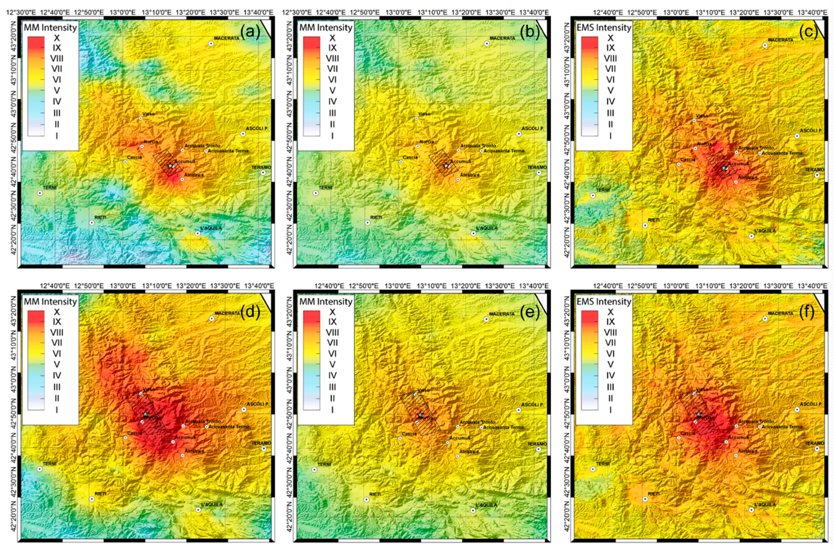
3.2. Maps of Macroseismic Intensity

Figure 8 shows the intensity maps for the MW 6.0 Amatrice earthquake obtained through the three relationships that referred to both CAV10 and AI. It is worth mentioning that CAB97 produces intensities in MSK scale, whereas KOL98 and T&D08 in MM scale, although Musson et al. [47] give a conversion between the two scales and EMS that indicates a substantial correspondence up to an intensity of X.
The CAB97 relationship based on CAV10 provides an area of 250 km2 with intensity ≥VIII and a very large area of about 16,400 km2 with a value ≥VI (Figure 8a). This prediction seems to strongly overestimate the area potentially damaged, given that in earthquake engineering practice, MM intensity VI is considered a reference point for earthquake damage, i.e., no damages occur to buildings of good design and construction for lower MM intensity. The other two CAV10-based relationships predict different scenarios with respect to the previous one. In fact, KOL98 (Figure 8c) and T&D08 (Figure 8e) highlight areas of 680 km2 and 525 km2 characterized by intensity ≥VIII between Amatrice and Norcia, towards SSE–NNW along the strike direction of the seismogenic source (see the dashed rectangle in Figure 8), and maximum intensity up to about IX close to the epicenter (white star in Figure 8) next to Accumuli village.
Generally, the AI-based maps show intensities lower than those obtained by CAV. CAB97 (Figure 8b) provides values in the epicentral area up to VII-VIII, whereas, KOL98 (Figure 8d) and T&D08 (Figure 8f) provide areas of 230 km2 and 500 km2 with intensity ≥VIII.
To summarize, it is possible to highlight that: (1) CAB97 provides a lack of agreement between maps as a function of the two ground-motion parameters, and instead; (2) a better agreement is shown by KOL98 and, even more, T&D08, especially in the most struck area; (3) the latter two relationships based on the same ground-motion parameter give similar results.
Figure 9, similar to the previous one, shows the intensity maps for the MW 6.5 Norcia earthquake.
As shown in the previous case, the CAB97 relationships (Figure 9a,b), moving away from the epicenter, provide very different intensities between them, and the maximum values in the more struck area are lower than those obtained by other models. Instead, the intensities based on CAV10 and AI show a greater agreement using KOL98 (Figure 9b,e) and, even more, T&D08 (Figure 9c,f). In fact, the area with intensity ≥VI is between 12,000 km2 and 14,500 km2 considering KOL98 or T&D08 based on both CAV10 and AI. In addition, the area characterized by intensity ≥VIII is 1810 km2 and 1981 km2 as predicted by T&D08 based on CAV10 or AI, respectively, and maximum intensities up to X are given for this earthquake.
According to the model depending both on the ground-motion parameters and the epicentral distance, as proposed by Tselentis and Danciu [29], the intensity maps are shown in Figure 10.
It should be noted that intensities predicted by these model are generally lower than those provided by previous relationships for both the Amatrice (Figure 10a,b) and Norcia earthquakes (Figure 10c,d). In particular, values quickly decrease from the maximum one that is provided in correspondence to the epicenter. This effect is due to the negative contribution of the increasing epicentral distance. The comparison between maps based on CAV and AI highlights similar intensity close to the epicenter, whereas, moving away from it, the CAV-based relationships furnish values slightly higher, generally.

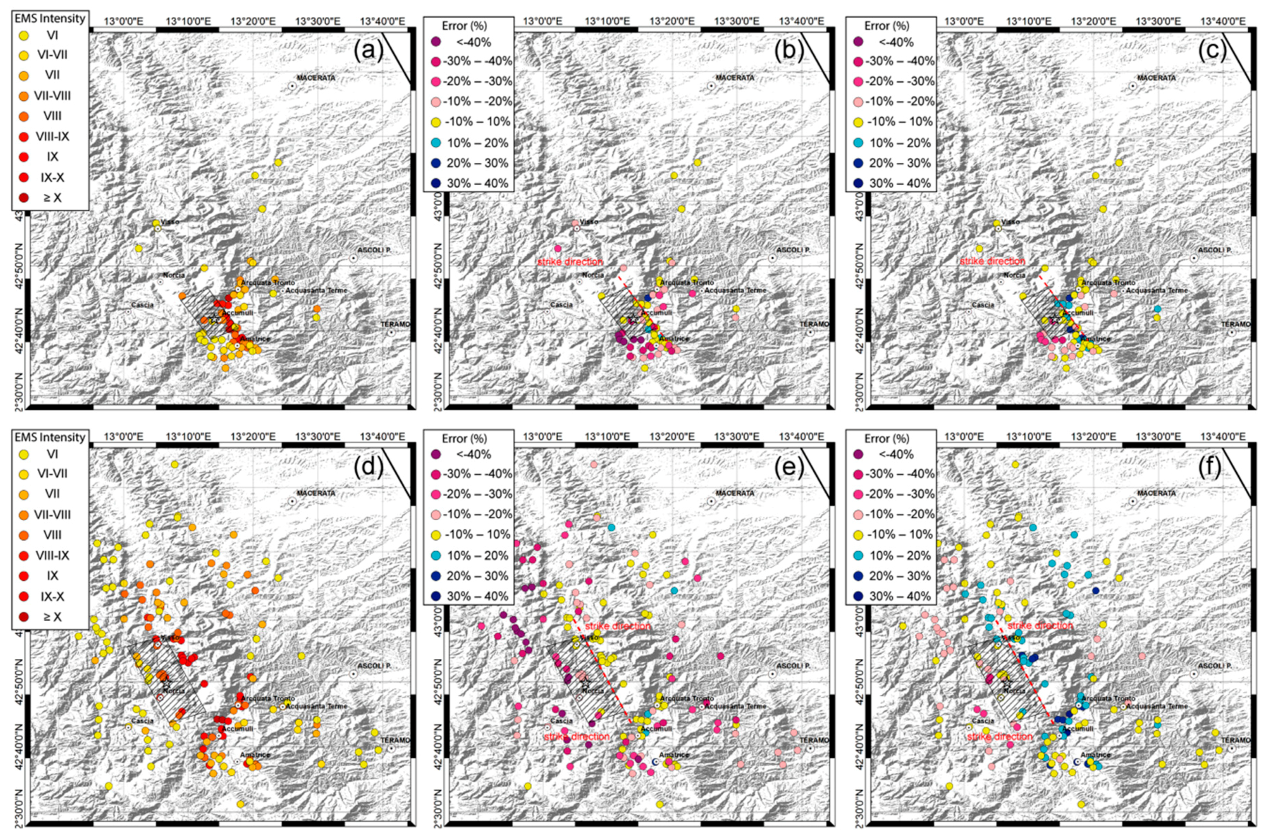
3.3. Comparison with Official ShakeMaps and Macroseismic Surveys

The results obtained by both models proposed by Tselentis and Danciu [29] are represented in Figure 11 as the mean of the intensities from CAV and AI—those only dependent on ground-motion parameters (Figure 11a,d) and, also, by epicentral distance (Figure 11b,e), each of them for the Amatrice and Norcia earthquakes, respectively. For the same geographical area, the official shaking maps (simply defined as ShakeMap below) according to Faenza and Michelini (2010, 2011) are shown for the two earthquakes (Figure 11c,f).
It should be kept in mind that intensity maps are expressed through the MM scale, whereas the official ShakeMaps refer to the MCS scale, although the conversion between the scales indicates a substantial correspondence up to an intensity of 10 [47].
The model that is only dependent on ground-motion parameters shows good agreement with the official maps for the highest intensity; in fact, normalized mean absolute gaps (which are calculated with an equation similar to Equation (14)) of 7% and 8% (for the two earthquakes) are associated to the intensity ≥VII. Instead, the same model shows a decreasing trend of the intensity which is more pronounced moving away from the epicenter with respect to the ShakeMaps. Contrariwise, the model dependent on the epicentral distance underestimates the intensities in most of the investigated area; in fact, the normalized absolute mean gaps in this case are 14% or 15% for intensity ≥VII.
Finally, the comparisons between the predicted and observed intensities (≥VI) are proposed in Figure 12. The observed intensities are those provided by the QUEST Group, which deals with carrying out macroseismic surveys immediately after a seismic event. This group made a first report on the effects of the Amatrice earthquake that occurred on 24 August 2016, [48] (cf. Figure 12a) and made updates following the subsequent severe shocks for the earthquakes of 26 and 30 October 2016 [49] (cf. Figure 12d). In the same figure, the comparisons between observed and predicted intensities are shown as normalized error in percentage (i.e., the difference between observation and prediction, in the same site, normalized with respect to the observation). The comparisons were performed for both the T&D08 model (Figure 12b,e), which only depends on ground-motion parameters, and the T&D08-2 model (Figure 12c,f), which also depends on the epicentral distance. The predicted intensities are the mean of those based on CAV and AI.
Keeping in mind the variability of the observed intensities, the trend of the errors seems to indicate different behaviors for the two models, especially when close to the epicenter. In fact, the T&D08 provides good agreement between predicted and observed intensities near the surface projection of the fault plane towards ENE from the strike direction (yellow circles close to the dashed red line in Figure 12b,e). Contrariwise, the same model overestimates the observed intensities towards WSW from the strike direction (cf. pink-purple circles close to the dashed red line in Figure 12b,e). It should be noted that negative values indicate predictions greater than the observed intensities, and vice versa. Opposite indications are given by the T&D08-2 model, which underestimates intensities towards ENE of the strike direction close to the fault plane (cyan-blue circles near the dashed red line in Figure 12c,f). In summary, the T&D08 model produces good predictions about the greater macroseismic intensities (cf. errors in Figure 12b,e correspond to red circles in Figure 12a,d, respectively) and it gives precautionary values, generally. Nevertheless, taking into account all data, T&D08-2 gives a better prediction with percentage errors mostly contained between −20% and 20% (about 83% of the observed intensities for both earthquakes). Probably, the differences between predicted and observed intensities close to the faults are also influenced by complex near-source effects (e.g., [50]). In addition, the underestimation of some predicted intensities with respect to those observed for the Norcia earthquake (positive errors in Figure 12f) could be affected by cumulative damage due to the moderate and severe earthquakes that occurred in the area within a few months.

4. Conclusions

In this paper, the author proposed a method to produce ground-motion shaking maps in terms of cumulative absolute velocity and Arias intensity and, thus, these were converted into intensity maps through some relationships available in literature.
An application of this procedure has been shown for the two strongest earthquakes of the seismic sequence that occurred in Central Italy between 2016 and 2017. Once the ground-motion parameters had been calculated on the basis of hundreds of horizontal recordings, kriging and cokriging geostatistical techniques with different models were compared for interpolation on the whole struck area. Additional calculation effort due to cokriging seems justified only for the first earthquake, for which the recordings in the epicentral area are limited and not spatially well-distributed. In the following phase, different relationships between intensity and ground-motion parameters were applied to obtain intensity shaking maps. The results obtained by models dependent only on ground-motion parameters were first analyzed, and afterwards, a model also dependent on epicentral distance was assumed.
The comparison with the official ShakeMaps showed a mean intensity in good agreement (and anyway, with precautionary values) in epicentral area applying the more recent models dependent only on the ground-motion parameters, whereas the model also dependent on epicentral distance produced lower intensities almost everywhere. Instead, the comparison with the observed macroseismic intensities (that obtained by field surveys) indicates that the models dependent only on ground-motion parameters well predict the greater intensities and overestimate the other ones, generally; whereas, when the model also dependent on epicentral distance is used, good agreement for most of the observations is found (83% of the data show an absolute percentage error lower than 20%), although the greater observed intensities (>IX) are generally underestimated.
The proposed procedure could be improved by the elaboration of new regression models of macroseismic intensity against the ground-motion parameters that are based on a more extended dataset, and probably by introduction of the local site effects, although this seems to not be strongly influential according to the proposed models. In addition, the near-source effects should be taken into account in the conversion of ground-motion parameters in intensity values.
Furthermore, rotation-invariant measures of the ground-motion parameters could be introduced in the interpolation process, in order to avoid any dependence on the orientation of the measuring sensors (e.g., [51]).
The first results obtained for the two specific earthquake scenarios look promising and this procedure could be used for rapid assessments of the damage framework on a large scale. It is worth emphasizing that the procedure should be used with care, keeping in mind the uncertainties dependent both on interpolation of ground-motion parameters and the relationships for predicting the macroseismic intensities.

Author Contributions

Antonio Costanzo is the only author.

Acknowledgments

The author thanks the three reviewers for their comments and suggestions, which were useful for improving the article.

Conflicts of Interest

The author declares no conflict of interest.

References

  1. De Rossi, M.S. Programma dell’osservatorio ed archivio centrale geodinamico presso il R. Comitato Geologico d’Italia. Bull. Vulcan. Ital. 1883, 10, 3–128. [Google Scholar]
  2. Sieberg, A. Geologie der Erdbeben. Handb. Geophys. 1930, 2, 552–555. [Google Scholar]
  3. Wood, H.O.; Neumann, F. Modified Mercalli intensity scale of 1931. Bull. Seismol. Soc. Am. 1931, 21, 277–283. [Google Scholar]
  4. Richter, C.F. Elementary Seismology; W H Freeman & Co.: San Francisco, CA, USA, 1958; 768p, ISBN 978-0716702115. [Google Scholar]
  5. Medvedev, S.; Sponheuer, W.; Karník, V. Neue seismische Skala (Intensity scale of earthquakes). In Proceedings of the 7th Symposium of the European Seismological Commission, Jena, Germany, 30 September 1962; Institut für Bodendynamik und Erdbebenforschung in Jena: Jena, Germany, 1964; Volume 77, pp. 69–76. [Google Scholar]
  6. Grünthal, G. European Macroseismic Scale 1998. In Chaiers du Centre Europèen de Gèodynamique et de Seismologie; Grünthal, G., Musson, R.M.W., Schwarz, J., Stucchi, M., Eds.; Conseil de l’Europe: Luxemburg, 1998; Volume 15, 100p, ISBN 2-87977-008-4. [Google Scholar]
  7. Wald, D.J.; Quintoriano, V.; Heaton, T.H.; Kanamori, H.; Scrivner, C.W.; Worden, C.B. TriNet “ShakeMaps”: Rapid generation of peak ground motion and intensity maps for earthquakes in southern California. Earthq. Spectra 1999, 15, 537–555. [Google Scholar] [CrossRef]
  8. Faenza, L.; Michelini, A. Regression analysis of MCS intensity and ground motion parameters in Italy and its application in ShakeMap. Geophys. J. Int. 2010, 180, 1138–1152. [Google Scholar] [CrossRef] [Green Version]
  9. Faenza, L.; Michelini, A. Regression analysis of MCS intensity and ground motion spectral accelerations (SAs) in Italy. Geophys. J. Int. 2011, 186, 1415–1430. [Google Scholar] [CrossRef] [Green Version]
  10. Wu, Y.M.; Teng, T.I.; Shin, T.C.; Hsiao, N.C. Relationship between peak ground acceleration, peak ground velocity and intensity in Taiwan. Bull. Seismol. Soc. Am. 2003, 93, 386–396. [Google Scholar] [CrossRef]
  11. Kaka, S.I.; Atkinson, G.M. Relationships between instrumental ground-motion parameters and modified Mercalli intensity in eastern North America. Bull. Seismol. Soc. Am. 2004, 94, 1728–1736. [Google Scholar] [CrossRef]
  12. Atkinson, G.M.; Kaka, S.I. Relationship between felt intensity and instrumental ground motion in the central United States and California. Bull. Seismol. Soc. Am. 2007, 97, 497–510. [Google Scholar] [CrossRef]
  13. Yaghmaei-Sabegh, S.; Tsang, H.H.; Nelson, T.K. Conversion between peak ground motion parameters and modified Mercalli intensity values. J. Earthq. Eng. 2011, 15, 1138–1155. [Google Scholar] [CrossRef]
  14. Pailoplee, S. Relationship between modified mercalli intensity and peak ground acceleration in Myanmar. Nat. Sci. 2012, 4, 624–630. [Google Scholar] [CrossRef]
  15. Worden, C.B.; Gerstenberger, M.C.; Rhoades, D.A.; Wald, D.J. Probabilistic relationships between ground-motion parameters and modified Mercalli intensity in California. Bull. Seismol. Soc. Am. 2012, 102, 204–221. [Google Scholar] [CrossRef]
  16. Bilal, M.; Askan, A. Relationships between Felt Intensity and Recorded Ground-Motion Parameters for Turkey. Bull. Seismol. Soc. Am. 2014, 104, 484–496. [Google Scholar] [CrossRef]
  17. Nemati, M. Relationships between Modified Mercalli Intensity and Engineering Ground-Motion of the Earthquakes in Persia. J. Earthq. Eng. 2016, 20, 795–808. [Google Scholar] [CrossRef]
  18. Panjamani, A.; Bajaj, K.; Moustafa, S.S.R.; Al-Arifi, N.S.N. Relationship between Intensity and Recorded Ground-Motion and Spectral Parameters for the Himalayan Region. Bull. Seismol. Soc. Am. 2016, 106, 1672–1689. [Google Scholar] [CrossRef]
  19. Bradley, B.A.; Bae, S.E.; Polak, V.; Lee, R.L.; Thomson, E.M.; Tarbali, K. Ground motion simulations of great earthquakes on the Alpine Fault: Effect of hypocentre location and comparison with empirical modelling. N. Z. J. Geol. Geophys. 2017, 60, 188–198. [Google Scholar] [CrossRef]
  20. Worden, C.B.; Wald, D.J. Shakemap Manual Online: Technical Manual, User’s Guide, and Software Guide. 2016. Available online: http://usgs.github.io/shakemap (accessed on 18 June 2018).
  21. Verros, S.A.; Wald, D.J.; Worden, C.B.; Hearne, M.; Ganesh, M. Computing spatial correlation of ground motion intensities for ShakeMap. Comput. Geosci. 2017, 99, 145–154. [Google Scholar] [CrossRef]
  22. Arias, A. A Measure of Earthquake Intensity. In Seismic Design for Nuclear Power Plants; Hansen, R.J., Ed.; MIT Press: Cambridge, MA, USA, 1970; Volume 1, pp. 438–469. ISBN 978-0262080415. [Google Scholar]
  23. Electrical Power Research Institute. EPRI. A Criterion for Determining Exceedance of the Operating Basis Earthquake; Report No. EPRI NP-5930; EPRI: Palo Alto, CA, USA, 1988. [Google Scholar]
  24. Electrical Power Research Institute (EPRI). Standardization of the Cumulative Absolute Velocity; EPRI TR-100082-T2; EPRI: Palo Alto, CA, USA, 1991. [Google Scholar]
  25. Campbell, K.W.; Bozorgnia, Y. Cumulative Absolute Velocity (CAV) and Seismic Intensity Based on the PEER-NGA Database. Earthq. Spectra 2012, 28, 457–485. [Google Scholar] [CrossRef]
  26. Baker, J.W.; Cornell, C.A. Vector-valued intensity measures for pulse-like near-fault ground motions. Eng. Struct. 2008, 30, 1048–1057. [Google Scholar] [CrossRef]
  27. Cabanas, L.; Benito, B.; Herraiz, M. An approach to the measurement of the potential structural damage of earthquake ground motions. Earthq. Eng. Struct. D 1997, 26, 79–92. [Google Scholar] [CrossRef]
  28. Koliopoulos, P.K.; Margaris, B.N.; Klims, N.S. Duration and energy characteristics of Greek strong motion records. J. Earthq. Eng. 1998, 2, 391–417. [Google Scholar] [CrossRef]
  29. Tselentis, G.A.; Danciu, L. Empirical relationships between modified Mercalli intensity and engineering ground-motion parameters in Greece. Bull. Seismol. Soc. Am. 2008, 98, 1863–1875. [Google Scholar] [CrossRef]
  30. Fiorentino, G.; Forte, A.; Pagano, E.; Sabetta, F.; Baggio, C.; Lavorato, D.; Nuti, C.; Santini, S. Damage patterns in the town of Amatrice after August 24th 2016 Central Italy earthquakes. Bull. Earthq. Eng. 2018, 16, 1399–1423. [Google Scholar] [CrossRef]
  31. Masi, A.; Chiauzzi, L.; Santarsiero, G.; Manfredi, V.; Biondi, S.; Spacone, E.; Del Gaudio, C.; Ricci, P.; Manfredi, G.; Verderame, G.M. Seismic response of RC buildings during the Mw 6.0 August 24 2016 Central Italy earthquake: The Amatrice case study. Bull. Earthq. Eng. 2017, in press. [Google Scholar] [CrossRef]
  32. Caserta, A.; Doumaz, F.; Costanzo, A.; Gervasi, A.; Thorossian, W.; Falcone, S.; La Piana, C.; Minasi, M.; Buongiorno, M.F. Assessing soil-structure interaction during the 2016 central Italy seismic sequence (Italy): Preliminary results. Ann. Geophys. 2016, 59, 1–7. [Google Scholar] [CrossRef]
  33. Michele, M.; Di Stefano, R.; Chiaraluce, L.; Cattaneo, M.; De Gori, P.; Monachesi, G.; Latorre, D.; Marzorati, S.; Valoroso, L.; Ladina, C.; et al. The Amatrice 2016 seismic sequence: A preliminary look at the mainshock and aftershocks distribution. Ann. Geophys. 2016, 59, 1–8. [Google Scholar] [CrossRef]
  34. Huang, M.H.; Fielding, E.J.; Liang, C.; Milillo, P.; Bekaert, D.; Dreger, D.; Salzer, J. Coseismic deformation and triggered landslides of the 2016 Mw 6.2 Amatrice earthquake in Italy. Geophys. Res. Lett. 2017, 44, 1266–1274. [Google Scholar] [CrossRef] [Green Version]
  35. Pucci, S.; De Martini, P.M.; Civico, R.; Villani, F.; Nappi, R.; Ricci, T.; Azzaro, R.; Brunori, C.A.; Caciagli, M.; Cinti, F.R.; et al. Coseismic ruptures of the 24 August 2016, Mw 6.0 Amatrice earthquake (central Italy). Geophys. Res. Lett. 2017, 44, 2138–2147. [Google Scholar] [CrossRef]
  36. Luzi, L.; Pacor, F.; Puglia, R. Italian Accelerometric Archive v 2.3. Istituto Nazionale di Geofisica e Vulcanologia. Dip. Prot. Civ. Naz. 2017. [Google Scholar] [CrossRef]
  37. Mucciarelli, M.; Gallipoli, M.R. Comparison between Vs30 and other estimates of site amplification in Italy. In Proceedings of the 1st European Conference on Earthquake Engineering and Seismology, Geneva, Switzerland, 3–8 September 2006.
  38. Gallipoli, M.R.; Mucciarelli, M. Comparison of site classification from VS30, VS10, and HVSR in Italy. Bull. Seismol. Soc. Am. 2009, 99, 340–351. [Google Scholar] [CrossRef]
  39. Isaaks, E.H.; Srivastava, M. Applied Geostatistics; Oxford University Press: New York, NY, USA, 1989; 561p, ISBN 978-0195050127. [Google Scholar]
  40. Webster, R.; Oliver, M.A. Geostatistics for Environmental Scientists, 2nd ed.; Wiley: Chichester, UK, 2007; 330p, ISBN 978-0470028582. [Google Scholar]
  41. Hengl, T. A Practical Guide to Geostatistical Mapping of Environmental Variables; Office for Official Publications of the European Communities: Luxembourg, 2007; 143p, ISBN 978-9279069048. [Google Scholar]
  42. Goovaerts, P. Geostatistics for Natural Resources Evaluation; Oxford University Press: New York, NY, USA, 1997; 483p, ISBN 978-0195115383. [Google Scholar]
  43. Jayaram, N.; Baker, J.W. Correlation model for spatially distributed ground-motion intensities. Earthq. Eng. Struct. Dyn. 2009, 38, 1687–1708. [Google Scholar] [CrossRef]
  44. Esposito, S.; Iervolino, I. PGA and PGV spatial correlation models based on European multievent datasets. Bull. Seismol. Soc. Am. 2011, 101, 2532–2541. [Google Scholar] [CrossRef]
  45. Du, W.; Wang, G. Intra-event spatial correlations for cumulative absolute velocity, Arias intensity, and spectral accelerations based on regional site conditions. Bull. Seismol. Soc. Am. 2013, 103, 1117–1129. [Google Scholar] [CrossRef]
  46. Wang, G.; Du, W. Spatial cross-correlation models for vector intensity measures (PGA, Ia, PGV and SAs) considering regional site conditions. Bull. Seismol. Soc. Am. 2013, 103, 3189–3204. [Google Scholar] [CrossRef]
  47. Musson, R.M.W.; Grünthal, G.; Stucchi, M. The comparison of macroseismic intensity scales. J. Seismol. 2010, 14, 413–428. [Google Scholar] [CrossRef] [Green Version]
  48. Galli, P.; Peronace, E.; Tertulliani, A. Rapporto Sugli Effetti Macrosismici del Terremoto del 24 Agosto 2016 di Amatrice in Scala MCS. Roma. Rapporto Congiunto DPC, CNR-IGAG e INGV. Available online: https://zenodo.org/record/161323#.Wyerh4p9hhE (accessed on 18 June 2018). (In Italian). [CrossRef]
  49. Tertulliani, A.; Azzaro, R. QUEST—Rilievo Macrosismico per i Terremoti Nell’Italia Centrale; Aggiornamento Dopo le Scosse del 26 e 30 Ottobre 2016. Aggiornamento al 21 dicembre 2016, rapporto interno INGV; Available online: https://zenodo.org/record/238778#.Wyer9Yp9hhE (accessed on 18 June 2018). (In Italian) [CrossRef]
  50. Luzi, L.; Pacor, F.; Puglia, R.; Lanzano, G.; Felicetta, C.; D’Amico, M.; Michelini, A.; Faenza, L.; Lauciani, V.; Iervolino, I.; et al. The Central Italy Seismic Sequence between August and December 2016: Analysis of Strong-Motion Observations. Seismol. Res. Lett. 2017, 88, 1219–1231. [Google Scholar] [CrossRef]
  51. Rupakhety, R.; Sigbjörnsson, R. Rotation-invariant mean duration of strong ground motion. Bull. Earthq. Eng. 2014, 12, 573–584. [Google Scholar] [CrossRef]
Figure 1. Configurations of the accelerometric seismic network during the two main events of the 2016–2017 Central Italy seismic sequence: on 24 August 2016, the MW 6.0 Amatrice earthquake (a), and on 30 October 2016, the MW 6.5 Norcia earthquake (b). Red stars are the epicenters (http://cnt.rm.ingv.it/) and dashed rectangles indicate the faults projected on the surface (http://shakemap.rm.ingv.it/).
Ijgi 07 00244 g001
Figure 2. Histograms of the engineering ground-motion parameters for MW 6.0 Amatrice earthquake (left panel) and MW 6.5 Norcia earthquake (right panel): standard cumulative absolute velocity with acceleration threshold of 10 cm/s2 (red bars), Arias intensity (green bars), peak ground acceleration (blue bars), and velocity (cyan bars). A natural logarithmic transformation was applied to all data.
Ijgi 07 00244 g002
Figure 3. Example of empirical semivariogram: original values together detrended ones and fitted models (a); detail on parameters for fitting a model (b).
Ijgi 07 00244 g003
Figure 4. Cross-validation between measured and predicted values through kriging (a,b) and cokriging (c,d) methods with the exponential fitting model for the MW 6.0 Amatrice earthquake. For the cokriging method, CAV10 and AI were selected alternatively as primary and the other one with PGA and PGV as secondary variables.
Ijgi 07 00244 g004
Figure 5. Cross-validation between measured and predicted values through kriging (a,b) and cokriging (c,d) methods with the exponential fitting model for the MW 6.5 Norcia earthquake. For the cokriging method, CAV10 and AI were selected alternatively as primary and the other one with PGA and PGV as secondary variables.
Ijgi 07 00244 g005
Figure 6. Cross-correlation between kriging and cokriging methods for CAV10 (a) and AI (b).
Ijgi 07 00244 g006
Figure 7. Interpolation of CAV10 and AI through the best-fitting models obtained for the MW 6.0. Amatrice earthquake (a,b) and the MW 6.5 Norcia earthquake (c,d). White stars are the epicenters (http://cnt.rm.ingv.it/) and dashed rectangles indicate the faults projected on the surface (http://shakemap.rm.ingv.it/).
Ijgi 07 00244 g007
Figure 8. Intensity maps for the MW 6.0 Amatrice earthquake based on cumulative absolute velocity (a,c,e) and Arias intensity (b,d,f). The maps were obtained by three different relationships: Cabanas et al. [27] (a,b), Koliopulos et al. [28] (c,d), and Tselentis and Danciu (2008) [29] (e,f).
Ijgi 07 00244 g008
Figure 9. Intensity maps for the MW 6.5 Norcia earthquake based on cumulative absolute velocity (a,c,e) and Arias intensity (b,d,f). The maps were obtained by three different models: Cabanas et al. [27] (a,b), Koliopulos et al. [28] (c,d), and Tselentis and Danciu (2008) [29] (e,f).
Ijgi 07 00244 g009
Figure 10. Intensity maps obtained through the model proposed by Tselentis and Danciu [29], which depend on the cumulative absolute velocity (a,c) or Arias intensity (b,d) and the epicentral distance: MW 6.0 Amatrice (a,b) and MW 6.5 Norcia earthquakes (c,d).
Ijgi 07 00244 g010
Figure 11. Comparison among intensity maps obtained according to the models proposed by Tselentis and Danciu [29] (a,b,d,e) and official ShakeMaps (c,f) according to Faenza and Michelini (2010), available online (http://shakemap.rm.ingv.it/shake/). The proposed maps obtained through T&D08 (a,d) and T&D08-2 (b,e) are the mean of those based on cumulative absolute velocity and Arias intensity for the MW 6.0 Amatrice (upper layer) and MW 6.5 Norcia earthquakes (lower layer).
Ijgi 07 00244 g011
Figure 12. Comparison among predictions and observations: intensities obtained by macroseismic surveys (a,d) (http://www.questingv.it/); percentage errors between the observed intensities and those predicted according to the both models proposed by Tselentis and Danciu [29], T&D08 (b,e) and T&D08-2 (c,f). Negative values indicate predictions greater than observed intensities, and vice versa. The predicted intensities are obtained as the mean of those based on cumulative absolute velocity and Arias intensity. Intensities and comparisons obtained for the MW 6.0 Amatrice (upper layer) and MW 6.5 Norcia earthquakes (lower layer) are reported.
Ijgi 07 00244 g012
Table 1. Indexes to assess accuracy of geostatistical prediction models for MW 6.0 Amatrice earthquake.
Geostatistical Method and ModelCAV10AI
NMAERMSER2NMAERMSER2
Kriging–Circular0.2242.6550.9390.2590.5420.933
Kriging–Spherical0.2252.6660.9380.2520.5320.933
Kriging–Exponential0.1872.2650.9560.2210.5060.934
Kriging–Gaussian0.3223.7770.8710.3700.6550.924
Kriging - Rational quadratic0.2713.2440.9050.3400.6060.927
CoKriging–Circular0.2222.9430.9450.2740.5070.934
CoKriging–Spherical0.2102.8440.9490.2240.4970.935
CoKriging–Exponential0.1251.8390.9740.2190.4930.935
CoKriging–Gaussian0.3344.0840.8950.3640.5880.927
CoKriging–Rational quadratic0.2303.2590.9400.2580.4970.934
NMAE is the normalized mean absolute error, RMSE is the root mean squared error, and R2 is the correlation coefficient. For more details, see Equations (14)–(16).
Table 2. Indexes to assess accuracy of geostatistical prediction models for MW 6.5 Norcia earthquake.
Geostatistical Method and ModelCAV10AI
NMAERMSER2NMAERMSER2
Kriging–Circular0.1274.7700.9790.1941.4870.976
Kriging–Spherical0.1284.8020.9790.1931.4810.978
Kriging–Exponential0.1184.4490.9820.1831.4150.978
Kriging–Gaussian0.27910.0920.9040.4293.4890.863
Kriging - Rational quadratic0.1977.4660.9470.3302.6390.929
CoKriging–Circular0.1315.2470.9750.1831.4240.977
CoKriging–Spherical0.1295.1670.9750.1831.4160.978
CoKriging–Exponential0.1124.4880.9830.1961.4750.978
CoKriging–Gaussian0.2328.6160.9280.3693.1360.896
CoKriging–Rational quadratic0.1716.6390.9580.2151.7280.970
NMAE is the normalized mean absolute error, RMSE is the root mean squared error, and R2 is the correlation coefficient. For more details, see Equations (14)–(16).

