Temporal and Spatial Analyses of the Landscape Pattern of Wuhan City Based on Remote Sensing Images

Abstract

With the acceleration of the process of building a national-level central city in Wuhan, the landscape pattern of the city has undergone tremendous changes. In this paper, remote images are classified through the neural network classification method, based on texture extraction, and the evolution of landscape patterns was quantitatively analyzed, based on the method of moving windows, landscape metrics and urban density calculation, in order to accurately extract landscape types and perform quantitative analyses. Wuhan City is taken as an example. The surface coverage of Wuhan City from 1989 to 2016 is divided into four types: agricultural landscape clusters, forest landscape clusters, water landscape clusters, and urban landscape clusters. It was concluded that, during the study period, the landscape heterogeneity of the entire area in Wuhan has increased, but the central urban area in Wuhan has decreased. The development of urban areas has compacted inwards but expanded outwards. In addition, the western part of Wuhan City developed better than the eastern part.

1. Introduction

With the rapid development of global technology and economy, global problems, such as increased urbanization and reduced biodiversity, have surfaced [1,2]. China has been in a period of rapid development in recent years, and the speed of urbanization in Wuhan, a national central city in China, is accelerating. The proportion of urban land-use types has been constantly changing in the total area of urban land, thereby affecting the entire landscape pattern and ecological processes of the city [3,4]. Therefore, the study of landscape patterns is extremely important for the urban planning and management of Chinese cities with rapid development.

Traditional landscape pattern analysis methods are mostly qualitative, analyzing the characteristics of the landscape pattern from the perspective of landscape ecology [5]. The most basic quantitative analysis method is spatial statistical analysis [6]. It analyses landscape changes by counting the area and proportion of various types of land. On this basis, several scholars have used the Markov transition matrix to analyze the loss direction of a certain type of land, and the source of a new type of land [7]. However, the accuracy of the traditional method was not high enough, and the results of the analysis greatly deviated from the actual situation [8].

With the development of remote sensing technology, some scholars have applied this technology to landscape pattern analysis [9]. Common methods for landscape classification are unsupervised classification and supervised classification [10]. Lillesand has experimentally pointed out that using hybrid classification (meaning a combination of supervised with unsupervised classification) to classify images can achieve higher classification accuracy [11]. Moreover, with the rise of neural networks, some scholars have used Back Propagation (BP) neural networks to classify images and achieve better results [12]. Based on this finding, McGarigal et al. have proposed a calculation method of landscape metrics [13], which is widely used in the analysis of landscape patterns, such as the urban landscape pattern [14], vegetation pattern [15], urban growth [16], and other subjects of study. Landscape metrics can quantitatively describe and monitor changes in landscape spatial structures over time, but it cannot specifically reflect the direction and rationality of landscape changes [17].

Jiao has proposed an “inverse S-shaped function” to formulate urban land density for urban land [18], which can identify the extent of the built-up area of Chinese cities and measure the compactness and expansion intensity of urban land. However, he only discusses the spatial distribution of urban land use, and does not analyze the changes in land-use structure during the development of a city. There are two problems in the current studies on landscape pattern. On the one hand, the interpretative features of images of different landscape types have been unclear, which has led to the prevalence of the “same object with different spectra, different objects with the same spectrum” phenomena [19]. On the other hand, most of these analyses are based on landscape metrics; this research method is relatively simple, and cannot reflect the complexity of the landscape pattern change in the rapid development process of Chinese cities [20].

Based on the above problems, this study combines remote sensing technology and an “inverse S-shaped function” model to quantitatively analyze the landscape pattern evolution of Wuhan from 1989 to 2016 from multiple angles. First, with the aim of improving the accuracy of image classification, we selected the texture features of the remote sensing image using the gray level co-occurrence matrix method, and construed a texture-based BP neural network model. Then, with the aim of analyzing the spatial and temporal characteristics of the landscape pattern in Chinese cities during the rapid development process, from the angles of landscape spatial characteristics, urban compactness, and development direction, etc., we have combined the methods of moving the window and the “inverse S-shaped function”.

2. Materials and Methods

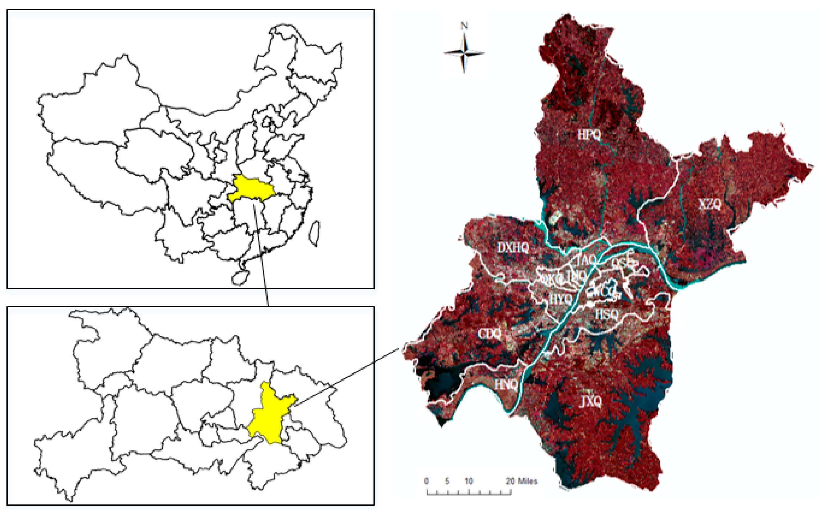
2.1. Study Area and Data

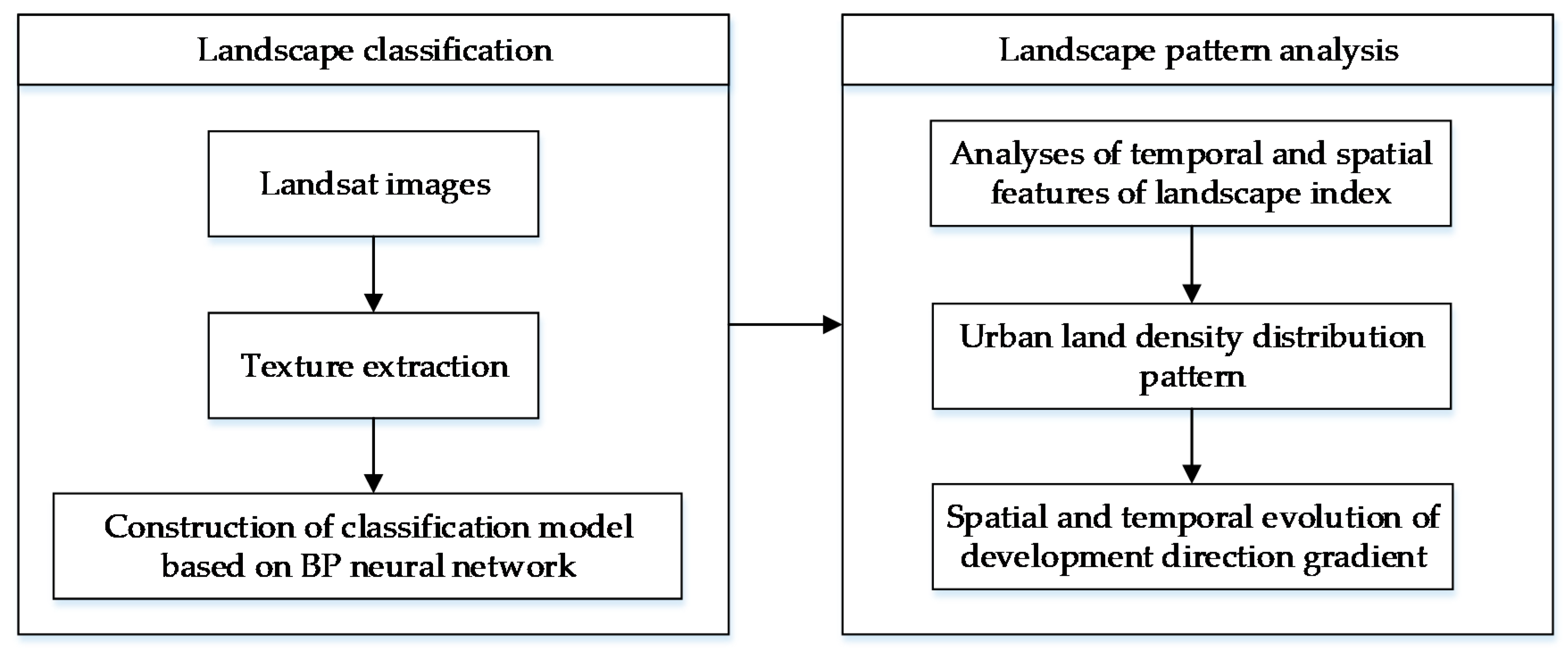
Wuhan is located in the Jianghan Plain, the central part of China and the eastern part of the Hubei Province. The elevation is less than 50 m in most areas of Wuhan. It is a national, historical, and cultural city, and an important industrial, scientific, and educational base in China.

From the statistical yearbook of Wuhan (http://www.whtj.gov.cn/), it is found that the built-up area of Wuhan has been expanding, and the population density has risen rapidly. As of 2017, the total built-up area had reached 719.85 km². From 1995 to 2017, the total population increased from 7.10 million to 10.77 million, which is an increase of 3.67 million, and the urbanization rate of permanent residents reached 79.3% in 2017. Moreover, since 1995, Wuhan’s economy has continued to grow rapidly. The gross national product grew from 60.69 billion RMB Yuan in 1995 to 1191.22 billion RMB Yuan in 2017, which is an average annual increase of 53.83 billion RMB Yuan.

Wuhan has played a leading role in the “1 + 8” urban circle, centered on Wuhan, and driven the economic and social development of the surrounding areas [21]. The advantages of its central position have brought policy and economic support to Wuhan. As a result, population, funds, and other resources gradually concentrate here under an agglomeration effect [22]. There are 13 jurisdictions in Wuhan, including seven central urban areas (Jiang’an District, Jianghan District, Qiaokou District, Qingshan District, Wuchang District, Hongshan District, and Hanyang District) and six suburbs (Dongxihu District and Hannan District are suburbs; Caidian District, Jiangxia District, Huangpi District, and Xinzhou District are far urban areas). This study focused on the 13 jurisdictions of Wuhan City.

The time period for this study was from 1989 to 2016. The Thematic Mapper (TM) images of Landsat-5 satellites and the Operational Land Imager (OLI) images of Landsat-8 satellites, with a resolution of 30 m, were used. The image data of the time series are shown in

Table 1. Image data.

Image Type	Acquisition Date (Month/Year)
Landsat-5	2/1989
	4/1995
	4/2001
	4/2004
	5/2007
	5/2010
Landsat-8	4/2013
	5/2016

. Three images were acquired at each time point, and the track numbers were 122/39, 123/38, and 123/39.

The Environment for Visualizing Images (ENVI) platform was used to do some preprocessing of images [23]. After preprocessing, the three images were inlaid according to the required research scope, and the administrative division data of Wuhan were then superimposed on them. Finally, the study area was cut, as shown in Figure 1, and bands 6, 4, and 3 were assigned to red, green, and blue, respectively, for synthesizing pseudo-color images.

2.2. Study Method

Based on the texture features extracted from the images, this paper establishes a BP neural network classification model to classify images in the study area. The temporal and spatial characteristics of landscape patterns were analyzed by selecting landscape indices, using moving windows, and calculating density curve methods. A technical flow chart is shown in Figure 2.

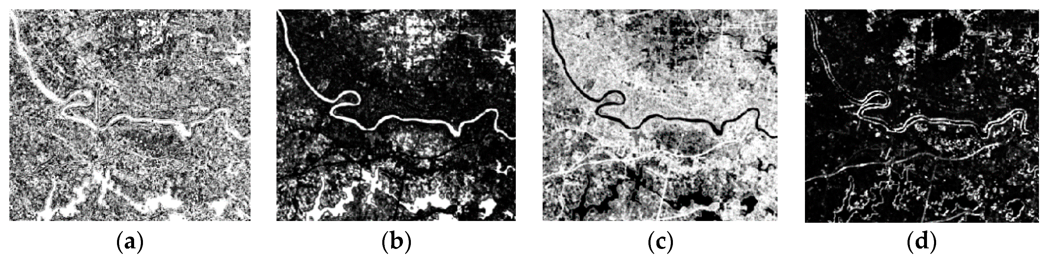
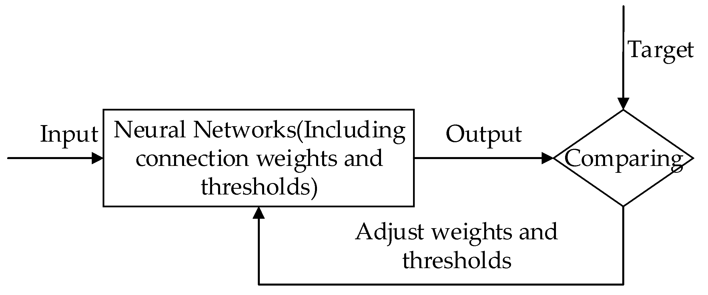
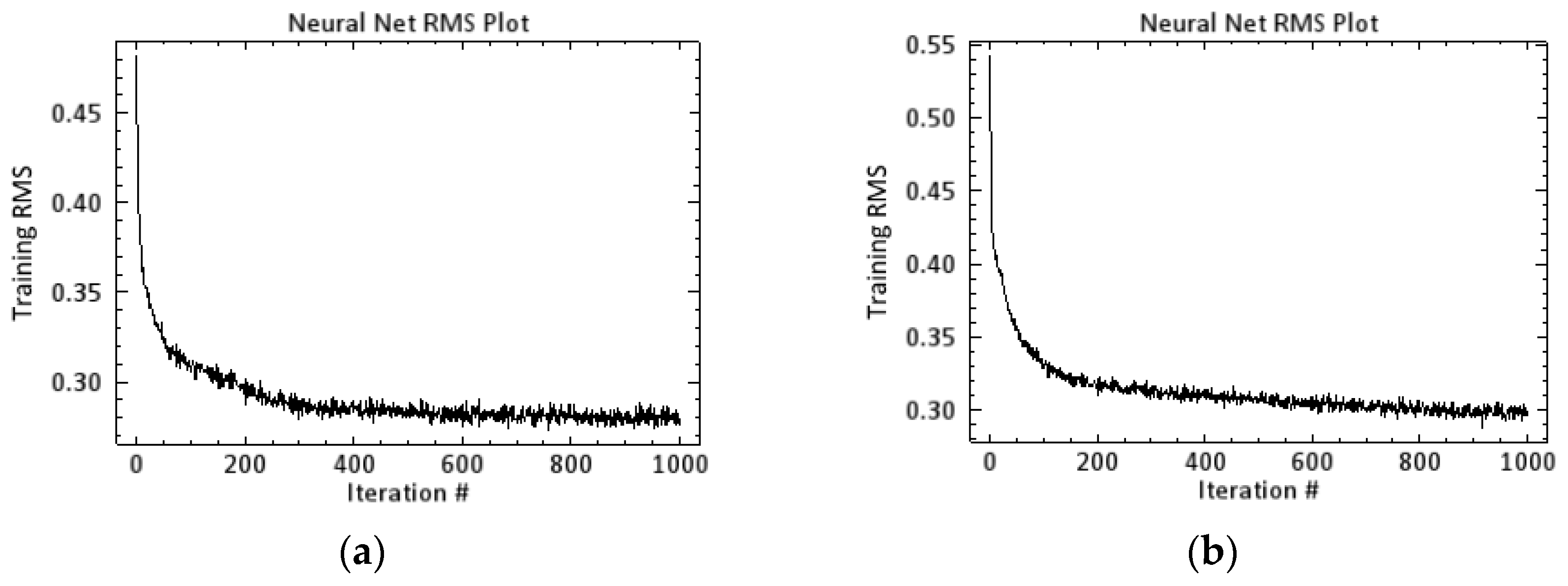
2.2.1. Texture-Based Back Propagation (BP) Neural Network Classification

The element with the lowest level in the landscape pattern system is the homogeneous landscape unit, and its upward classification complies with the relationship between the natural bodies and landscape units of similar neighboring natural landscapes [24,25]. Based on the principle of landscape classification, and combined with the research data and purposes, the landscape of the overall Wuhan area is divided into the following clusters (landscape clusters are an organic combination of multiple similar landscape functional areas):

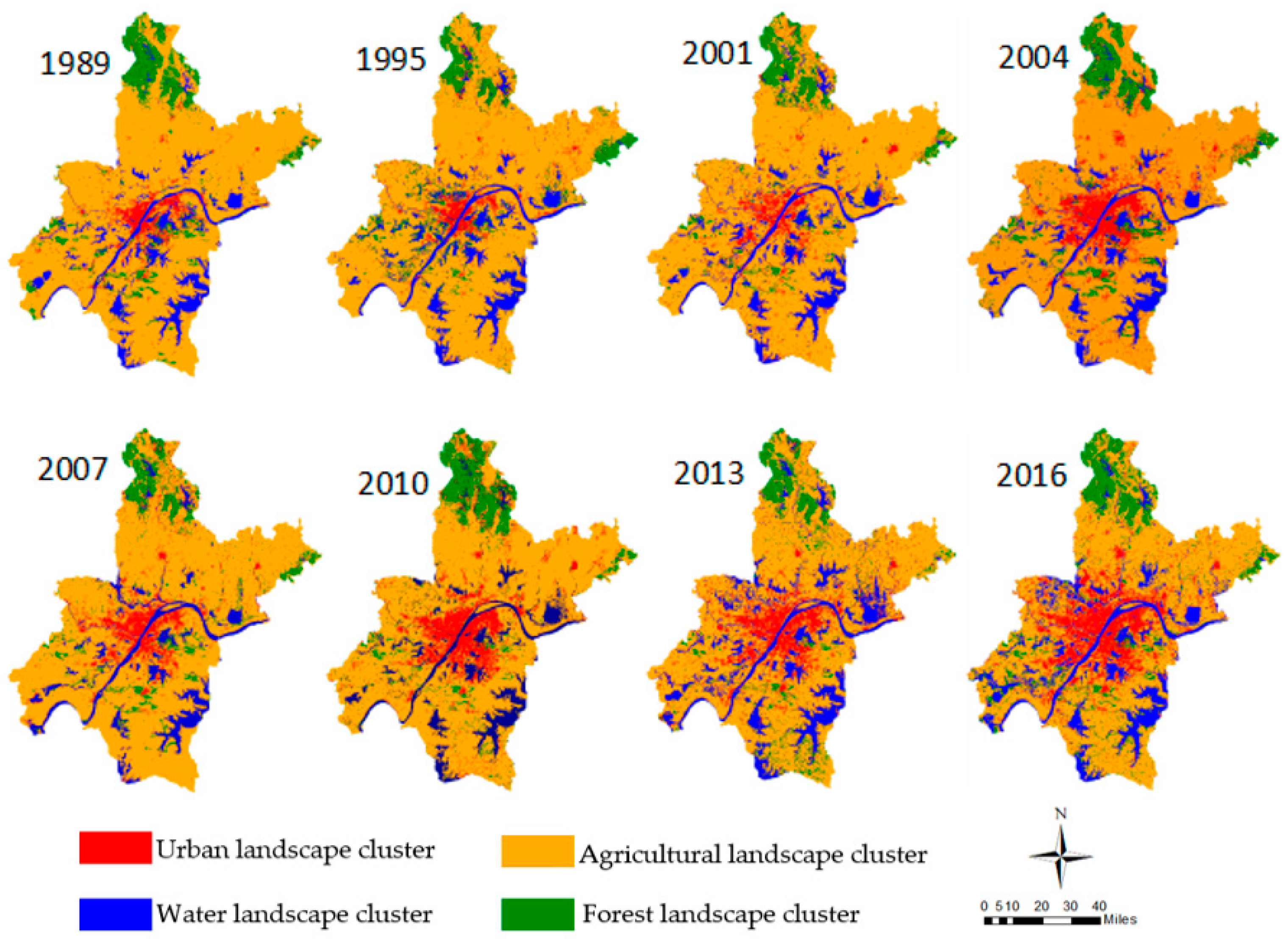
• Forest landscape cluster, including landscape units such as woodland, garden, and grassland.
• Agricultural landscape cluster, including landscape units such as dry land and vegetable plots.
• Water landscape cluster, including landscape units such as the Yangtze River, lakes, and rivers.
• Urban landscape cluster: including landscape units, such as houses, roads, and rural settlements.

In this paper, the gray level co-occurrence matrix (GLCM) method was used to extract the texture features of the images of Wuhan City [26]. The GLCM starts from a pixel at a certain position A(x, y) in the image, and counts the probability P(i, j, δ, θ) of the occurrence of pixels (x + ∆x, y + ∆y) whose image has a gray value of j in a circular range, with a distance of δ from A. The mathematical formula was

$$\begin{array}{l}P(i,j,\delta ,\theta )=\{[(x,y),(x+\Delta x,y+\Delta y)]f(x,y)=i\\ f(x+\Delta x,y+\Delta y)=j;x=0,1,2\cdot \cdot \cdot ,N_X-1;y=0,1,2\cdot \cdot \cdot ,N_y-1\}\end{array}$$

(1)

where x and y were the pixel coordinates in the image; and N_x and N_y were the number of rows and columns of the images, respectively.

Haralick has defined 14 kinds of texture feature parameters from four aspects: statistical characteristics, characteristics of information theory, characteristics of correlation, and characteristics of visual texture [26]. The gray level co-occurrence matrix can measure various information in the image, and the feature image can visually display the thickness of the texture and the characteristics of each direction. Common statistical features are entropy, contrast, energy, and correlation. By extracting the texture features, the phenomena of the “same object with different spectra, different objects with the same spectrum” can be better solved, which helps to improve the classification accuracy of images.

Since there was still a certain correlation between the bands, in order to reduce the time and amount of calculation of neural network training, the fifth band (with the most abundant surface information) and the red band of visible light were selected after the principal component analysis (PCA). Finally, the images with the texture features of contrast (CON), angular second moment (ASM), entropy (ENT), and correlation (COR) were extracted (Figure 3).

Based on the extracted texture features, this paper used a BP network model with only one hidden layer for classification. The input layer of the neural network was six multi-spectral bands and eight texture images. The output layer was six initial classification categories and one other category. The transfer function (i.e., the activation function) of the hidden layer and output layer adopted a logarithmic logic to achieve a highly nonlinear mapping from the input to the output layer. The basic principle diagram of neural network training is shown in Figure 4. For the training of the BP neural network, it was necessary to determine several important parameters in the training model, including training contribution threshold (c), training momentum (m), training rate (r), network global error (e), and number of training iterations (n).

This study has selected many group parameters for comparison experiments. The error curve of neural network training, under various parameter settings, is shown in Figure 5. Figure 5a is a set of settings with good training results after multiple tests, and Figure 5b is the default set of settings, recommended by the system. It is found that the training time is about 4 h when the parameter settings are those shown in Figure 5a, whereas, when the parameter settings are those used in Figure 5b, the training time is about 5 h. Moreover, the final training error in the group illustrated in Figure 5a is lower than that in of the group shown in Figure 5b, so this study chooses the parameter settings demonstrated in Figure 5a.

2.2.2. Analytical Method of Landscape Metrics

Landscape metrics is a measure that quantitatively represents the composition of the landscape pattern and the spatial form or distribution of different landscape types [27]. FRAGSTATS computes three levels of metrics, corresponding to (1) each patch in the mosaic, (2) each patch type (class) in the mosaic, and (3) the landscape mosaic as a whole [13]. Landscape metrics are large in number, although the repeatability and correlation of the landscape information contained in the metrics are high [28]. It is very important to select appropriate metrics for the study. In this paper, the patch density (PD) and Shannon diversity index (SHDI) of the landscape level were selected based on the regional features of Wuhan and the study objective.

1. Patch density (PD)

Patch density represents the patch number of one specific landscape type per one-hundred-hectare area. The formula is:

$$\mathrm{PD}=\frac{{\mathrm{N}}_{\mathrm{i}}}{\mathrm{A}}$$

(2)

The PD value can reflect the fragmentation degree of the landscape in the study area [29]. The larger the patch number per unit area, the higher the fragmentation degree of the landscape in the area.

2. Shannon diversity index (SHDI)

Heterogeneity refers to the degree of confounding of different types of landscapes within the region [30]. A high degree of confounding indicates that the distribution of different types of landscapes is balanced and has strong heterogeneity [30]. If a certain type of landscape in a region is shown to be superior, the landscape pattern in the region is unbalanced and the heterogeneity is low, which is not conducive to the ecological development of the region [31]. The Shannon diversity index (SHDI) represents the heterogeneity of the landscape in the study area. The formula is:

$$\mathrm{SHDI}=-{\displaystyle \sum }_{i=1}^m\left(P_i\ln P_i\right)$$

(3)

The range of SHDI values is SHDI ≥ 0. The larger the SHDI, the greater the mixing degree and heterogeneity of patch types, so the distribution of patch types became more and more balanced in the landscape.

Based on the calculation results of the selected landscape metrics, the landscape pattern was further analyzed using the moving window method. The moving window method is used to calculate the landscape metrics selected in the “calculation window”, and output the corresponding raster map to observe the spatial variability of the landscape pattern. In addition, this method could clarify the information from the landscape spatial pattern [32]. In comparison with traditional analyses, which are based on overall features, using the moving window method for performing spatial gradient analysis in landscape pattern could realize the quantification and spatial visualization of the landscape metrics in the local area, and thereby more clearly exhibit the dynamic spatial change of the landscape pattern and reveal the differences in the internal structure of the landscape [33].

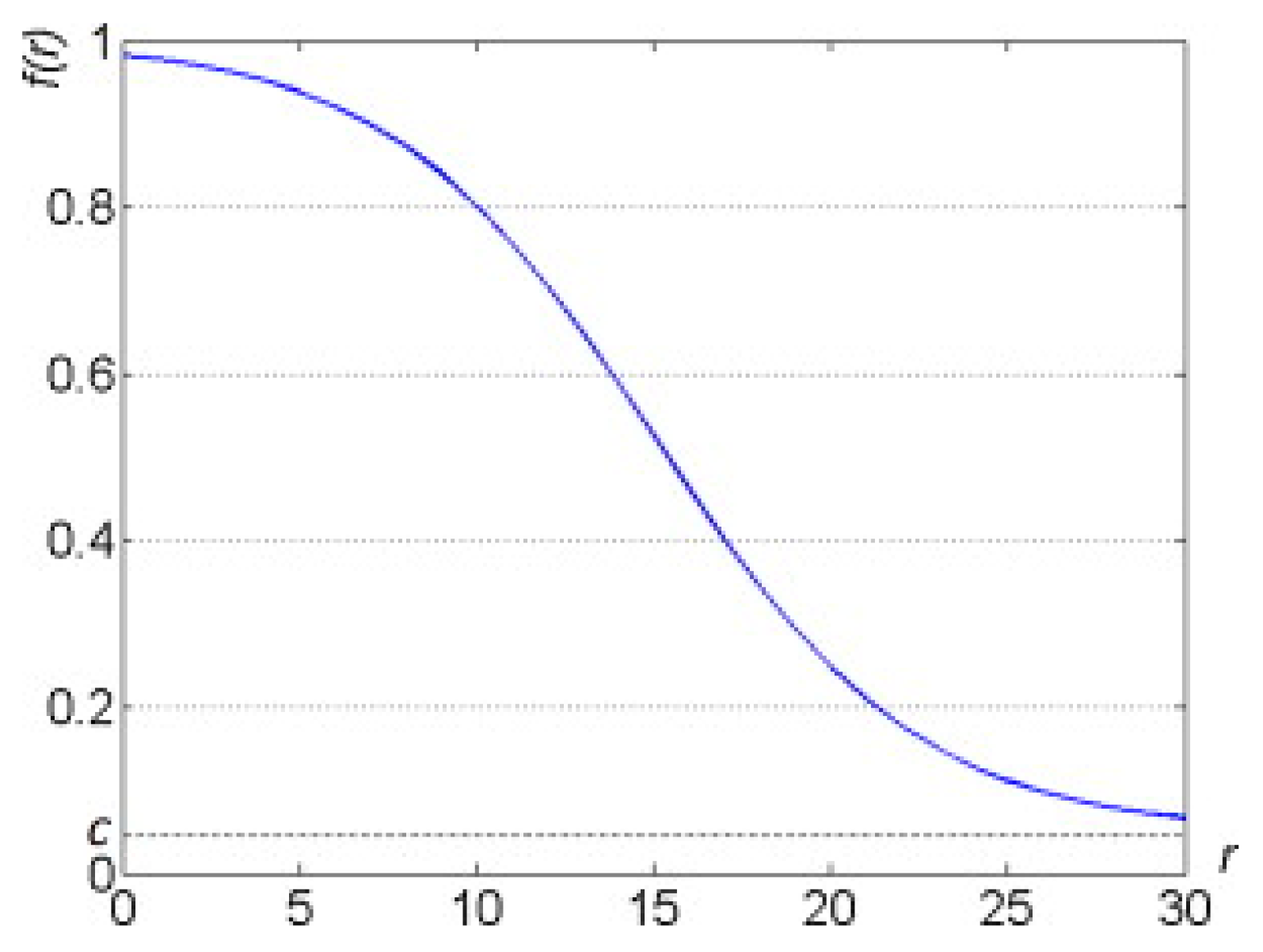
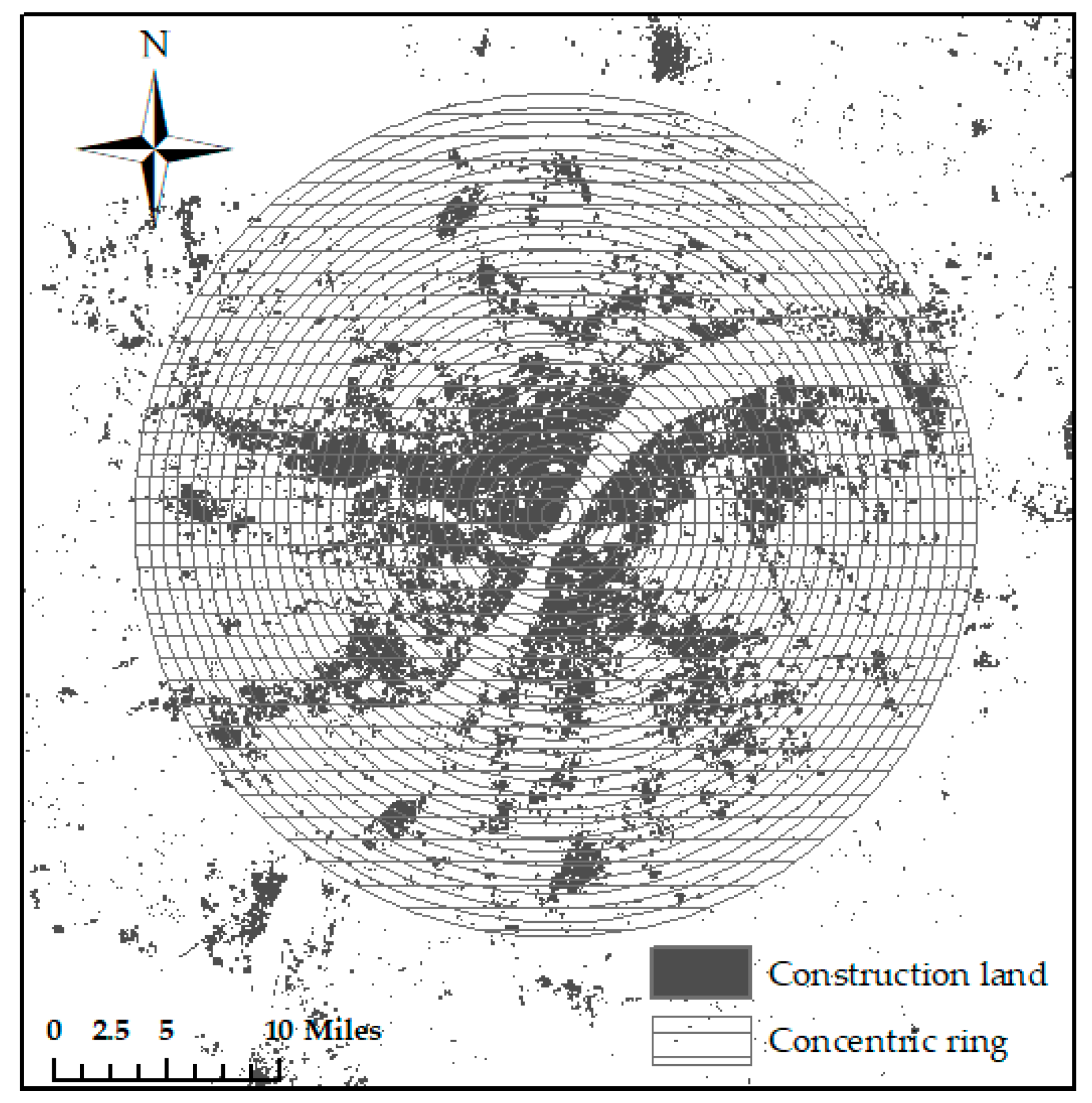
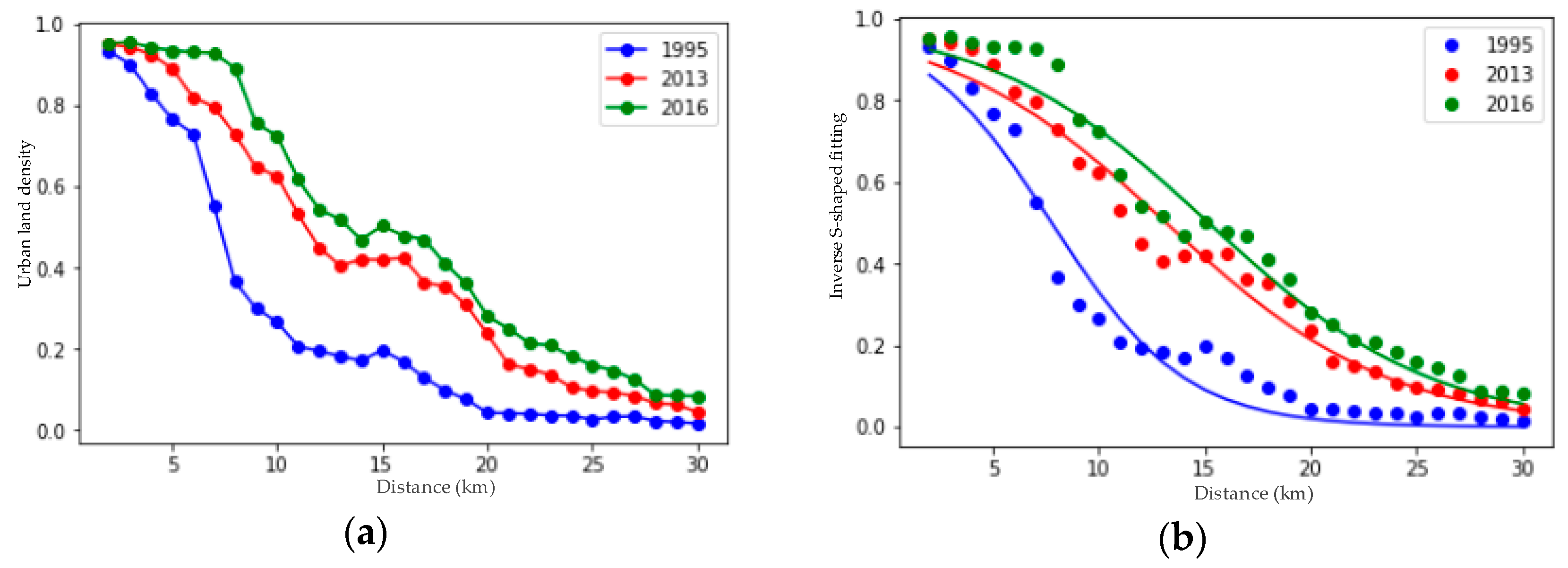
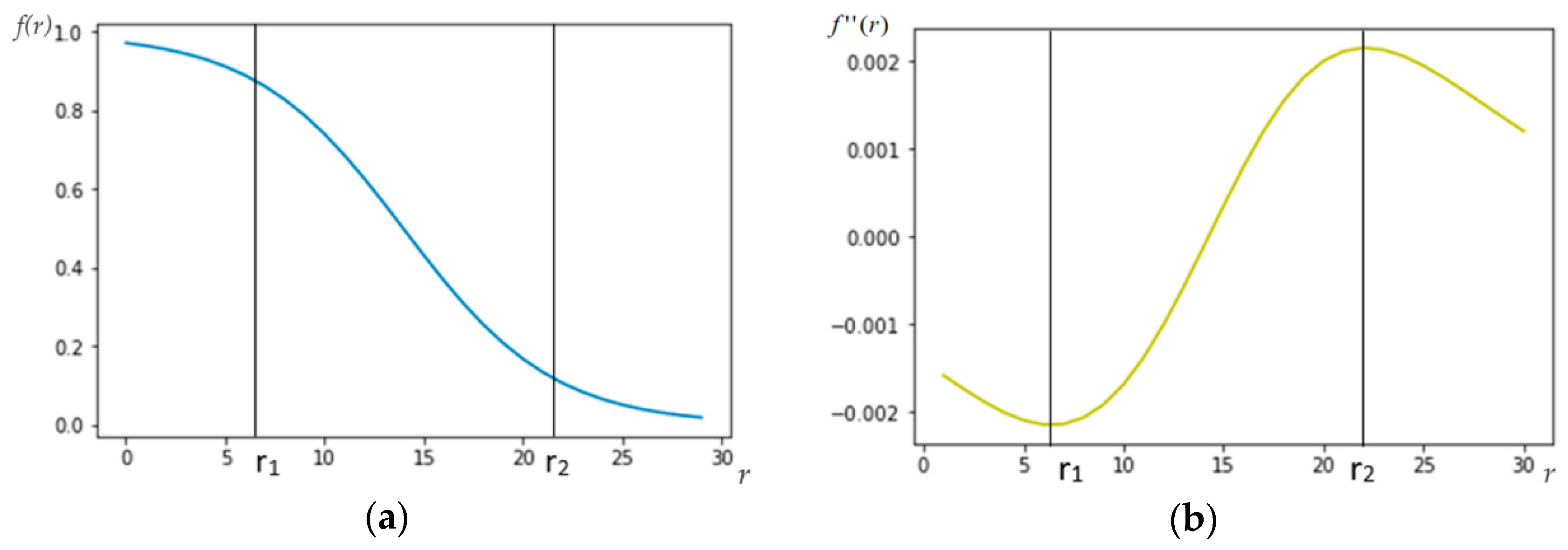
2.2.3. Urban Density Curve

Urban density analyses have always been the focus in the study of urban expansion. This paper used the concentric circles division method to calculate the urban land use density of each ring [18]. Then, the spatial variation regularity of urban land use was analyzed, based on the relation between urban land use density variation and the distance from the urban center.

The least square method is used to fit the inverse S-shaped function of urban land use, based on Python. The formula is

$$\mathrm{f}\left(\mathrm{r}\right)=\frac{1-\mathrm{c}}{1+{\mathrm{e}}^{\mathsf{\alpha }(\frac{2\mathrm{r}}{\mathrm{D}}-1)}}$$

(4)

where f is urban density, r is the distance from the urban center, e is the Euler value, α, c, and D are constants, and D is the maximum radius of the urban center.

The function form, when α = 4, c = 0.05, and D = 30, is shown in Figure 6. The urban land density function is a continuously monotonic decreasing differentiable function. It has two horizontal asymptotes, f = 1 and f = c. When r = 0 (representing the urban center), f(r) is close to 1; when r approaches infinity, f(r) is close to c.

3. Results

The Kappa coefficient of image classification results is shown in

Table 2. Calculation results of Kappa coefficient.

Year	1989	1995	2001	2004	2007	2010	2013	2016
Kappa coefficient	0.8854	0.8063	0.7924	0.7928	0.8178	0.8056	0.8236	0.8389

. The classification results meet the requirements of the accuracy of this research. The results are shown in Figure 7.

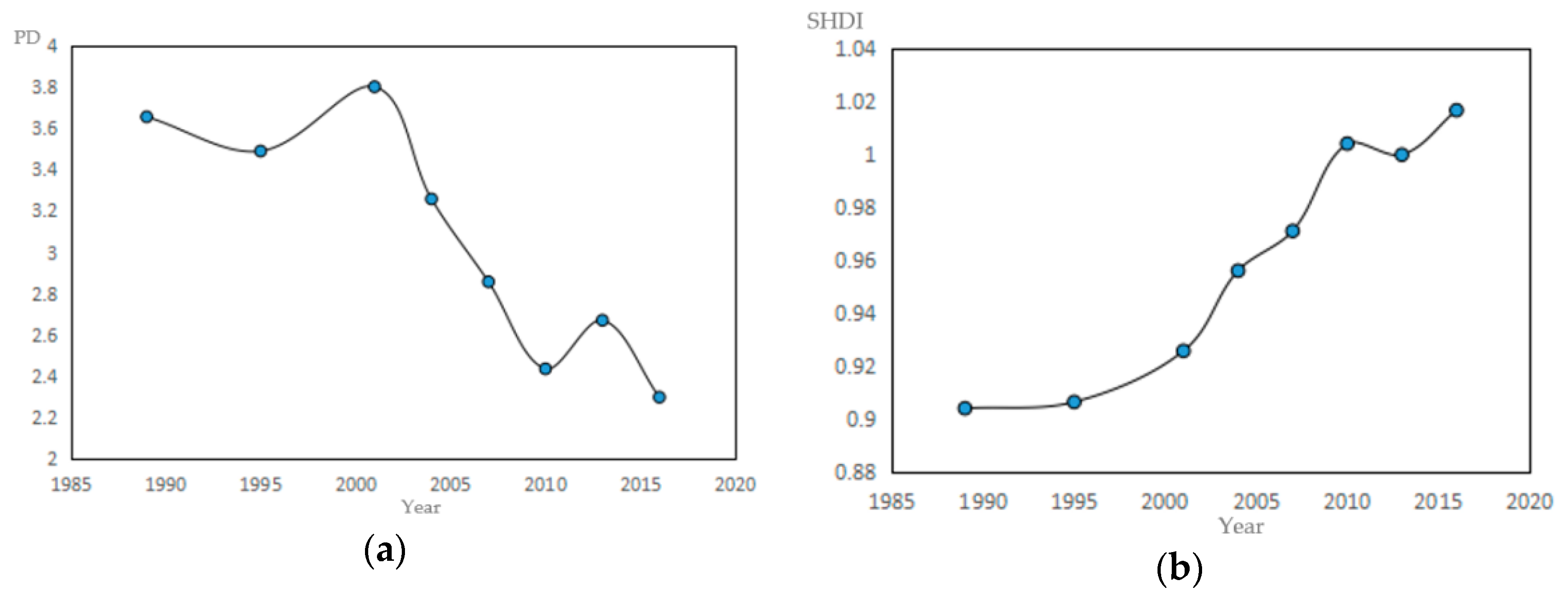
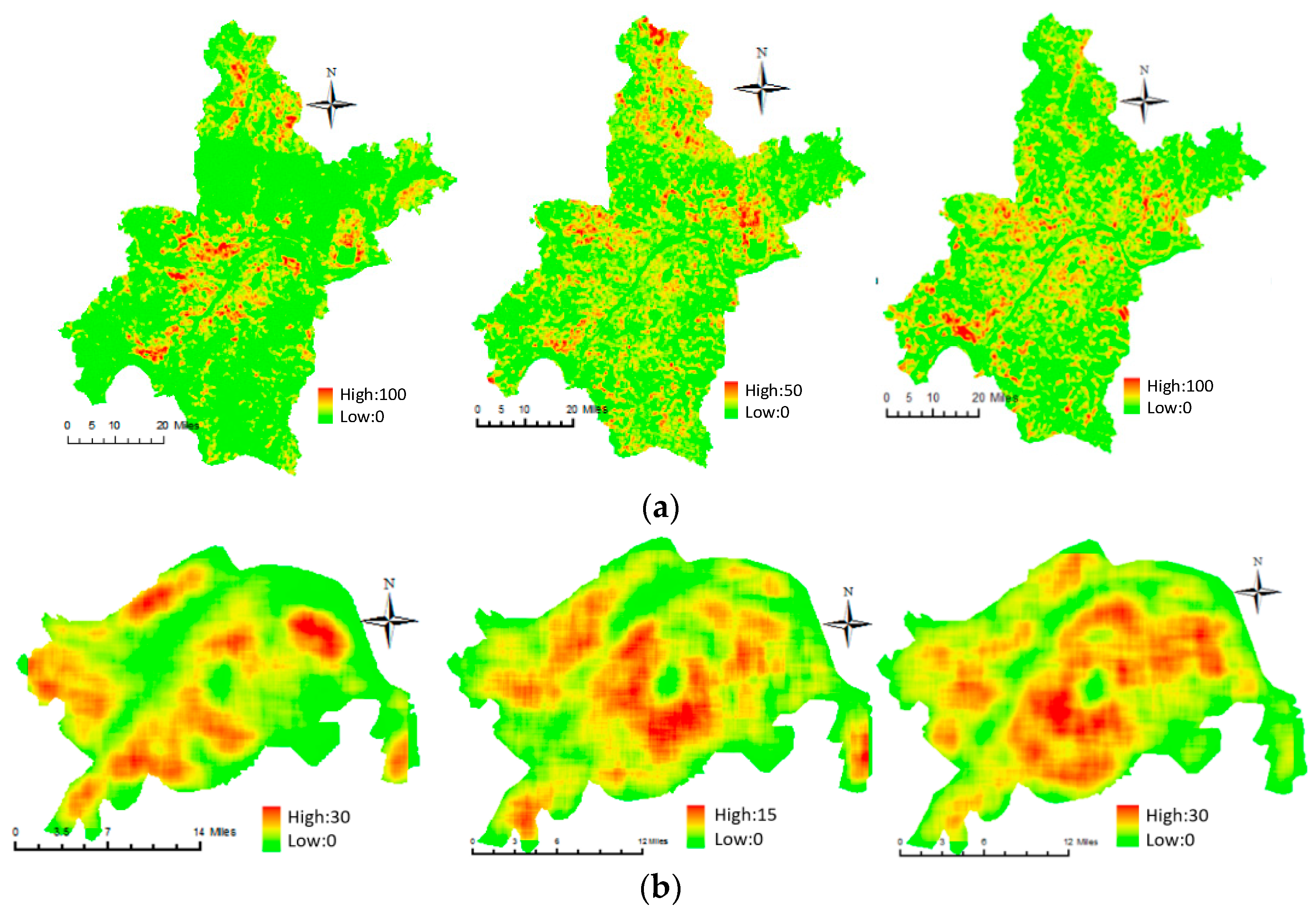
3.1. Analyses of the Temporal and Spatial Features of Landscape Metrics

The patch density (PD) and Shannon diversity index (SHDI), at the landscape level, can reflect the basic spatial features of the landscape pattern, such as the fragmentation degree and heterogeneity [34]. The calculation results of PD and SHDI of the entire area in Wuhan are shown in

Table 3. Patch density (PD) and Shannon diversity index (SHDI) calculation results at the landscape level.

Year	PD	SHDI
1989	3.6556	0.904
1995	3.4896	0.9064
2001	3.801	0.9257
2004	3.2578	0.956
2007	2.8566	0.971
2010	2.4352	1.004
2013	2.6703	0.9998
2016	2.2976	1.0166

. The variation trend of PD and SHDI is shown in Figure 8. From 1989 to 2016, the PD of the landscapes of Wuhan showed a decreasing trend, but SHDI showed an increasing trend.

Patch density (PD) reflects the fragmentation degree of the landscape in the research area. Based on the calculation results of PD, this paper first analyzes the fragmentation degree of the landscape in Wuhan City. In order to specifically analyze the landscape changes in different areas of Wuhan, the moving windows method was adopted from the upper left corner of the research area at two scales, 1 km and 3 km. Then, the calculated values were assigned to the center grid of the window. The PDs, on the landscape level of the entire city (1 km scale) and the city center (3 km scale), were calculated separately (Figure 9).

As shown in Figure 9a, in 1995, the areas with a higher patch density were distributed in the concentrated downtown periphery: Southern Huanghua, Northern Xinzhou, and Eastern Hannan. Since the central urban area of Wuhan was covered by a large area of contiguous construction land, the patch density was relatively low (shown as large green), but the fragmentation degree of the city periphery, neighboring farmland, waters, and villages, had increased to a relevant degree. By 2013, the green area in the city center, with a low degree of fragmentation, had increased to a relevant degree, indicating that the land use of the city center had become more compact, and the fragmentation degree of the red area, between urban and rural areas, had been reduced to a relevant degree. By 2016, the areas with a high degree of fragmentation still included the Zhangdu Lake periphery, Central Dongxihu District, and Eastern Hannan District. In addition, the degree of fragmentation of the Eastern Hannan District had increased to a relevant degree. That was because the Eastern Hannan District is at the junction of agricultural landscape clusters, urban landscape clusters, water landscape clusters, and forest landscape clusters, so landscape types quickly transformed.

As shown in Figure 9b, the patch density in the downtown area decreased by 53% from 1995 to 2013, because the smaller architectural patches were connected and merged into larger patches as a result of city development. However, the patch density of the Southern and Northern Hongshan District increased to a relevant degree, indicating a rapid landscape transformation. Due to the rapid development of the Guanggu area, the degree of fragmentation in 2016 became higher when compared to that in 2013 (an overall increase of 42%).

The SHDI can be used to measure landscape heterogeneity. Based on the calculation results of the SHDI, this paper analyzes the heterogeneity of the landscape in Wuhan. During the study period, the SHDI of Wuhan showed an overall upward trend. The distribution of the landscape patterns in Wuhan had generally become more balanced. The SHDI calculation results, at the landscape level of the whole city (1 km scale) and the city center (3 km scale), are shown in Figure 10.

As shown in Figure 10a, the overall landscape of Wuhan became more and more balanced as the city expanded and developed. The original large-scale agricultural landscape clusters were broken into small pieces and transformed into other types of landscape clusters. By 2016, the SHDI index of the city periphery had increased by 21% compared to that in 1995, and the area with a high index became larger. As shown in Figure 10b, the SHDI metrics in the city center showed a declining trend from 1995 to 2016. This was the inevitable result of the development of the city center [35]. The landscapes of other types continuously transformed into urban landscape clusters. The heterogeneity of the central urban area of Wuhan decreased.

3.2. Urban Land Density Distribution Pattern

Wuhan is divided into three parts by the Yangtze River and Han River. Due to the special geographical locations of Wuhan, in this paper, the geometric center of the three old districts, where commerce has been concentrated, was selected as the circle center, and the main urban area of Wuhan was divided into thirty rings, one every kilometer, as shown in Figure 11. In order to eliminate the impact of large water bodies, such as the Yangtze River and East Lake, the water portion of each ring was removed before the land use density in each ring was calculated. The results are shown in Figure 12a. The fitting curve of urban land use density in 1995, 2013, and 2016 is shown in Figure 12b.

The density of urban land was high in the compact city, but low in the area around the city center. Therefore, the density curve was steep for the compact city, but gentle for the expanded city. The slope of the function curve of urban land use density could be used to reflect the total density of urban land use. The slope of the sharply descending part of the curve was used to reflect the compactness of the city. As shown in Figure 13, compactness was defined as the ratio between the difference value of the radius that corresponded to the minimum and maximum value of the second derivative of the fitting curves, and the maximum radius. This difference value was $\mathrm{k}=({\mathrm{r}}_2-{\mathrm{r}}_1)/\mathrm{D}$ [18].

Previous research points out that a compact city generally has a narrow area that includes the inner city and suburbs. The difference between r₁ is r₂ was small, so the k value is small [36]. On the other hand, a city with a large k value is a low-density or decentralized city [37]. The fitting parameter values and calculated k values of Wuhan from 1989 to 2016 are shown in

Table 4. Calculation results.

Year	α	c	D	k
1989	2.479	0.036	15.554	0.53
1995	2.493	0.041	18.528	0.48
2001	2.486	0.033	19.733	0.50
2004	2.481	0.029	22.672	0.44
2007	2.496	0.022	25.468	0.41
2010	2.507	0.021	26.732	0.39
2013	2.510	0.019	28.354	0.36
2016	2.894	0.006	30.366	0.31

. It can be seen that the value of k gradually decreases. By 2016, the value of k was reduced by 41.5%, and the development of the central urban area became more and more compact.

At the same time, for the fitted density function of urban land, the D parameter was an estimated value of the radius of the main urban area [18]. The increase of D indicated urban growth. As shown in Table 4, from 1989 to 2016, the D value for Wuhan increased from 15.554 to 30.336, indicating that the distance from the urban boundary to the urban center increased from 15.554 km to 30.336 km. The variation of the D value of Wuhan over the past 20 years is shown in Figure 14a. It can be seen that the urban area rapidly expanded, especially from 2000 to 2016. In Figure 14b, the red represented the construction land in 1989 and gray represented the construction land in 2016. The circle represents the expansion of the urban boundary from 1989 (inner layer) to 2016 (outer layer). Clearly, during the study period, the urban area of Wuhan expanded significantly.

The results showed that, on the one hand, the commercial and political centers of Wuhan were still in the three old urban areas—Wuchang, Hankou, and Hanyang—during the study period, which promoted the development of the entire urban area. As a result, the development pattern tended compact inwardly. On the other hand, due to the rapid economic development of Wuhan and the continuous adjustment of the industrial structure, the construction land of old urban areas could not meet the requirements of industrial and commercial construction. The central urban area rapidly expanded to nearby suburbs.

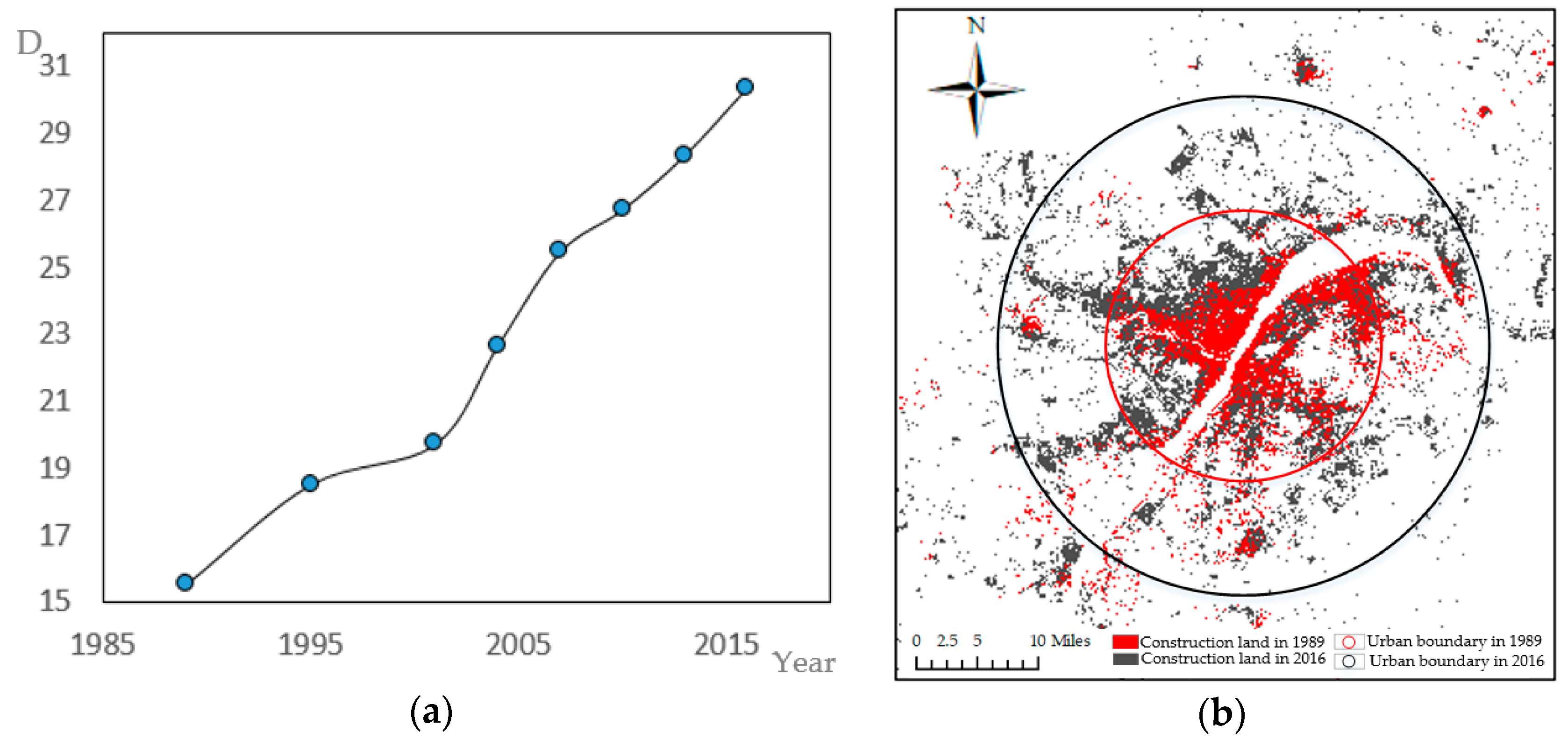
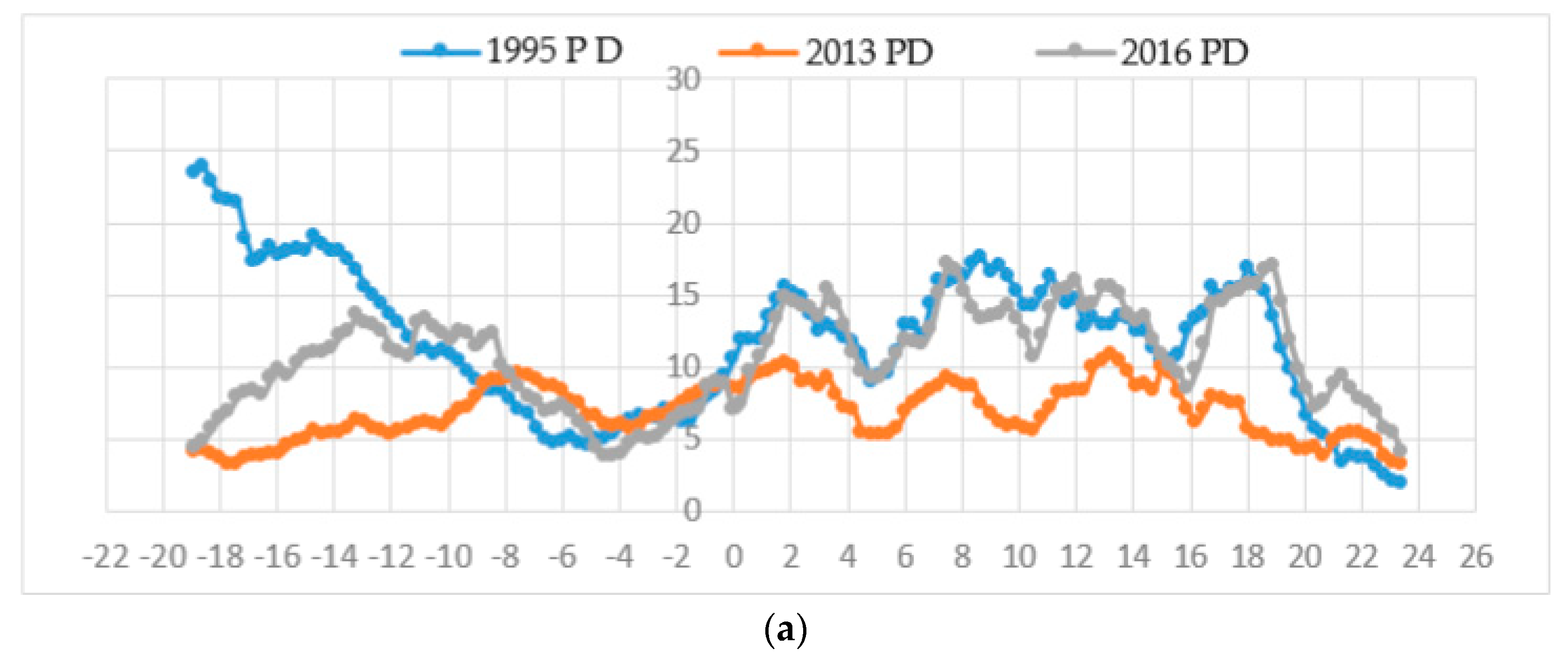
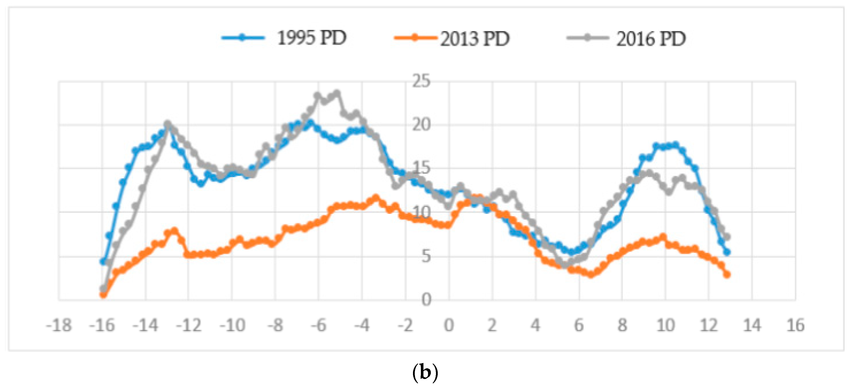
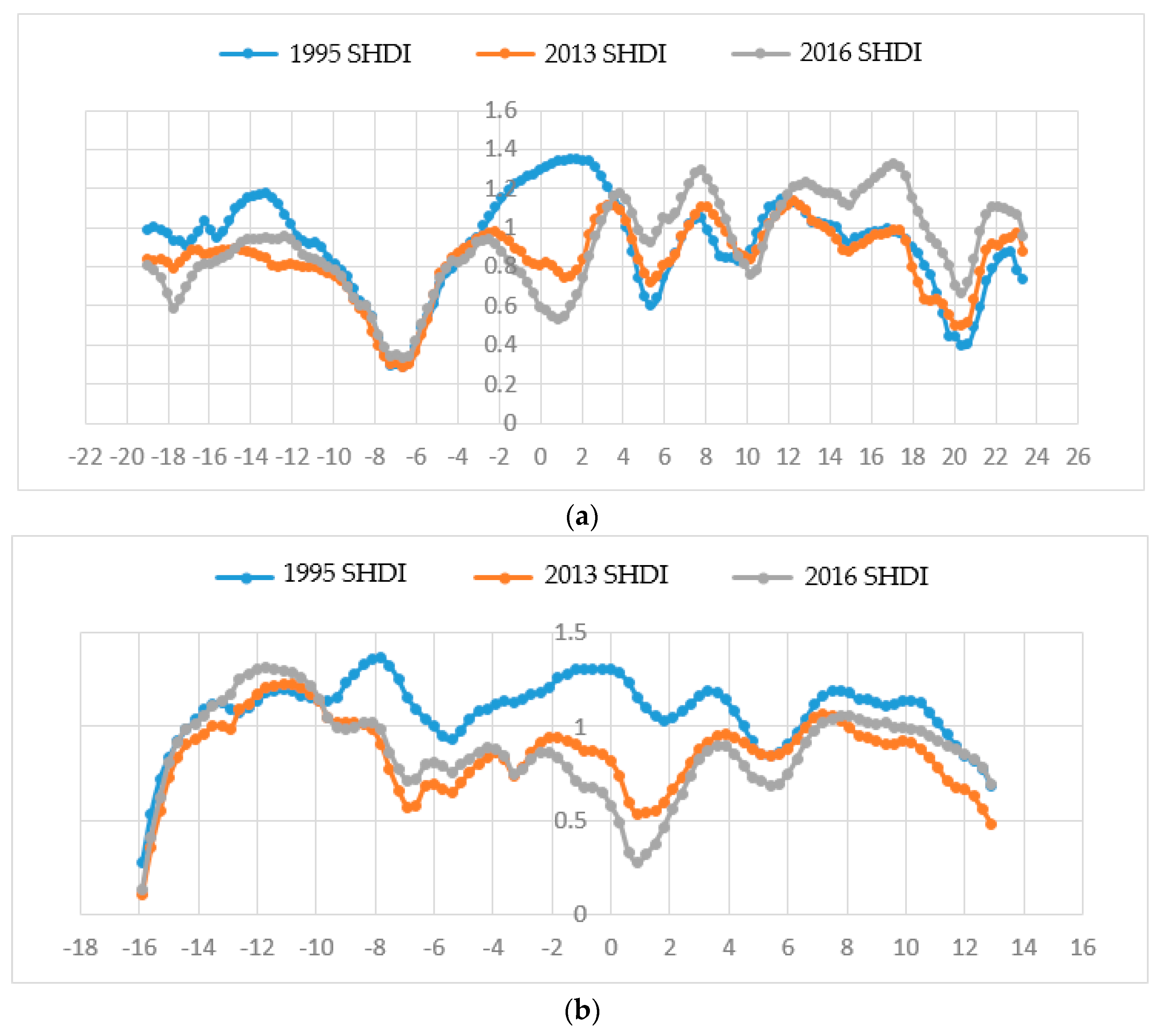
3.3. Spatial and Temporal Evolution of the Development Direction Gradient

In this study, samples were collected from the center of Wuhan to the East, West, South, and North, with an interval of 300 m, in order to explore the development direction of the central urban areas of Wuhan. There were a total of 142 sampling points in the eastern and western directions, and a total of 92 sampling points in the South and North directions. Samples were collected in the spatial distribution maps of 1995, 2013, and 2016, in order to acquire the distribution map of the PD and SHDI values, with the variation in the distance from the urban center (Figure 15 and Figure 16).

It could be concluded from Figure 15 that in 1995, the maximum PD value appeared in the West, about 19 km away from the urban center. The PD rapidly decreased, with the distance changing from 19 km to 6 km in the West (a decrease of 70.3%). This was the transition from the urban–rural border to the urban center. From 2013 to 2016, the PD value, ranging between 19 km and 14 km, decreased significantly (a reduction of 48% on average). This indicated that the urban–rural boundary expanded outward, and that the PD value of the original urban–rural boundary decreased. From the urban center to the East, the PD values for the three years had a similar variation trend. There were two fragmentation peaks at 10 km and 12 km away from the urban center, at the junction of a lake and construction land, indicating the destructive effect of urban expansion on the water landscape cluster. Overall, the difference in the West was greater than that in the East, indicating that Wuhan expanded more quickly westward than it did eastwards.

It could be concluded from Figure 16 that the SHDI values of 1995, 2013, and 2016 had the same variation trend in the East, West, South, and North. The SHDI metrics represented a declining trend at the junction of urban and rural areas, 16–19 km west of the urban center. The small patches on the urban margin continuously merged into large clusters. The boundary of Sand Lake was 1 km to the east of the urban center, where the SHDI value was reduced by 61%. This was because the area of Sand Lake was continuously shrinking and transforming into urban construction land. Fengshan forest reserve was east of the urban center. Due to proper protection measures, the SHDI was almost unchanged. In the north–south direction, the SHDI in 2013 was reduced more significantly than it was in 1995 (a reduction of 31.3%). but was slightly lower than it was in 2016 (a reduction of 8.6%). Agriculture, water, and forest landscape clusters transformed into construction land due to the industrial and commercial development in Qingshan District and Hongshan District. Therefore, the uniformity of the landscape was reduced.

4. Discussion and Conclusions

This paper proposes a landscape classification method based on texture, and a multi-angle landscape analysis method based on landscape metrics, urban land use density, etc. The challenges faced during urbanization, such as an increased degree of urban fragmentation and a decrease of connectivity, were effectively analyzed. Moreover, our study results can provide a scientific and effective technique, as well as data support for the construction of ecological cities and the optimization of urban spatial layouts [38]. In this paper, a texture-based BP neural network classification model has been constructed by extracting texture features, which improved the accuracy of image classification. This paper also introduced similar function classification methods from landscape ecology, and the landscape of Wuhan was classified into multiple clusters, including forest landscape, water landscape, urban landscape, and agricultural landscape clusters. Finally, we analyzed three aspects of the landscape pattern: the temporal and spatial features of landscape metrics, the urban land density distribution pattern, and the spatial and temporal evolution of the development direction gradient.

Moreover, two main conclusions can be extracted from this paper. Firstly, the heterogeneity of different landscape types in the entire area in Wuhan increased. However, the landscape types were unevenly distributed, and the heterogeneity of landscape patterns decreased as a result of the rapid development of the central urban area. The degree of fragmentation of the urban and rural boundary was higher than that of the central urban area. The landscape metrics of the western part was more intense than that of the eastern part. The development in the West was better than that in the East. Secondly, the compactness of Wuhan was quantitatively calculated by fitting the inverse S-curve based on the urban land use density. During the study period, the k value was reduced from 0.53 to 0.31, indicating that the development tended to compact inward. At the same time, the expansion status of the urban areas of Wuhan was quantitatively analyzed by calculating the urban radius D. Wuhan expanded outwards.

Since many landscape metrics coincide in measuring landscape features, we have only selected two metrics that can reflect the changes in landscape characteristics. In future studies, more landscape metrics, such as the effective mesh size, Euclidean nearest neighbor, or interspersion index, should be used to identify changes in urban spatial structures more accurately. According to the results of analyses of the urban landscape pattern of Wuhan, the study methods and procedures in this paper had good applicability. In future planning and development of Wuhan, the protection of cultivated land and forest land should be strengthened to prevent the continuous reduction of the forest and farmland landscape. At the same time, durin the process of urban expansion, we should pay attention to the matching and connection of various landscapes. The contradictions between man and land that emerge during the rapid expansion of urban areas should be reduced, in order to ensure the rationality and ordering of the landscape structure. In this way, Wuhan can effectively exert the radiation effect of the central urban area, and promote the balanced development and harmonious progress of the Wuhan Urban Circle.

References

1. Roders, A.P. How can urbanization be sustainable? A reflection on the role of city resources in global sustainable development. BDC–Bollettino del Centro Calza Bini 2014, 13, 79–90. [Google Scholar]
2. Bhatta, B.; Saraswati, S.; Bandyopadhyay, D. Urban sprawl measurement from remote sensing data. Appl. Geogr. 2010, 30, 731–740. [Google Scholar] [CrossRef]
3. Xiao, D. On the Formation and Development of Modern Landscape Science. Sci. Geogr. Sin. 1999, 19, 379–384. [Google Scholar]
4. Wu, J. Landscape Ecology—Patterns, Processes, Scales, and Ranks, 2nd ed.; Higher Education Press: Bejing, China, 2007. [Google Scholar]
5. Xiao, D.; Zhong, L.S. Ecological principles of landscape classification and assessment. Chin. J. Appl. Ecol. 1998, 9, 217–221. [Google Scholar]
6. Brandt, J. Landscape ecological information through statistical analysis of the territorial structure of a sheep grazing system, Faroe Islands. In Proceedings of the First International Seminar on Methodology in Landscape Ecological Research and Planning of the International Association for Landscape Ecology (IALE), Roskilde, Denmark, 15–19 October 1984. [Google Scholar]
7. Pan, D.; Domon, G.; Blois, S.D.; Bouchard, A. Temporal (1958–1993) and spatial patterns of land use changes in Haut-Saint-Laurent (Quebec, Canada) and their relation to landscape physical attributes. Landsc. Ecol. 1999, 14, 35–52. [Google Scholar] [CrossRef]
8. Veldkamp, A.; Verburg, P.H. Modelling land use change and environmental impact. J. Environ. Manag. 2004, 72, 1. [Google Scholar] [CrossRef] [PubMed]
9. Verburg, P.H.; Soepboer, W.; Veldkamp, A.; Limpiada, R.; Espaldon, V.; Mastura, S.S. Modeling the spatial dynamics of regional land use: The CLUE-S model. Environ. Manag. 2002, 30, 391. [Google Scholar] [CrossRef] [PubMed]
10. Kitada, K.; Fukuyama, K. Land-Use and Land-Cover Mapping Using a Gradable Classification Method. Remote Sens. 2012, 4, 1544–1558. [Google Scholar] [CrossRef] [Green Version]
11. Lillesand, T.M. Remote Sensing and Image Interpretation; Wiley: Hoboken, NJ, USA, 2006. [Google Scholar]
12. Ke, H.M.; Chen, C.Z.; Zhang, X.H.; Wang, J.L. Study on BP neural network classification with optimization of genetic algorithm for remote sensing imagery. J. Southwest Univ. 2010, 38, 157–166. [Google Scholar]
13. Mcgarigal, K.; Marks, B.J. FRAGSTATS: Spatial analysis program for quantifying landscape structure. Gen. Tech. Rep. PNW 1995, 122, 351. [Google Scholar]
14. Bai, X.; Shi, P.; Liu, Y. Society: Realizing China’s urban dream. Nature 2014, 509, 158–160. [Google Scholar] [CrossRef] [PubMed]
15. Wang, L.; Tian, B.; Koike, K.; Hong, B.; Ren, P. Integration of Landscape Metrics and Variograms to Characterize and Quantify the Spatial Heterogeneity Change of Vegetation Induced by the 2008 Wenchuan Earthquake. ISPRS Int. Geo-Inf. 2017, 6, 164. [Google Scholar] [CrossRef]
16. Dahal, K.R.; Benner, S.; Lindquist, E. Urban hypotheses and spatiotemporal characterization of urban growth in the Treasure Valley of Idaho, USA. Appl. Geogr. 2017, 79, 11–25. [Google Scholar] [CrossRef]
17. Lechner, A.M.; Reinke, K.J.; Wang, Y.; Bastin, L. Interactions between landcover pattern and geospatial processing methods: Effects on landscape metrics and classification accuracy. Ecol. Complex. 2013, 15, 71–82. [Google Scholar] [CrossRef]
18. Jiao, L. Urban land density function: A new method to characterize urban expansion. Landsc. Urban Plan. 2015, 139, 26–39. [Google Scholar] [CrossRef]
19. Wang, H.; Guo, J.; Ma, Z. Monitoring Wheat Stripe Rust Using Remote Sensing Technologies in China; Springer: Berlin, Germany, 2012. [Google Scholar]
20. Defries, R.S.; Asner, G.P.; Houghton, R.A. Landscape Level Analysis of the Spatial and Temporal Complexity of Land-Use Change; American Geophysical Union: Washington, DC, USA, 2013; pp. 217–230. [Google Scholar]
21. He, J.; Li, C.; Yu, Y.; Liu, Y.; Huang, J. Measuring urban spatial interaction in Wuhan Urban Agglomeration, Central China: A spatially explicit approach. Sustain. Cities Soc. 2017, 32, 569–583. [Google Scholar] [CrossRef]
22. Chen, Z.; Zhang, A.; Shan, X. Urbanization and administrative restructuring: A case study on the Wuhan urban agglomeration. Habitat Int. 2016, 55, 46–57. [Google Scholar] [Green Version]
23. Coulter, L.L.; Stow, D.A.; Tsai, Y.H.; Ibanez, N.; Shih, H.C.; Kerr, A.; Benza, M.; Weeks, J.R.; Mensah, F. Classification and assessment of land cover and land use change in southern Ghana using dense stacks of Landsat 7 ETM+ imagery. Remote Sens. Environ. 2016, 184, 396–409. [Google Scholar] [CrossRef]
24. Li, X.Q.; Zhou, L.; Sun, Z.; Song, Y. Analysis on changes of landscape pattern of Shenyang City assisted by TM images. Ecol. Sci. 2016, 35, 79–84. [Google Scholar]
25. Fan, Q.; Ding, S. Landscape pattern changes at a county scale: A case study in Fengqiu, Henan Province, China from 1990 to 2013. Catena 2016, 137, 152–160. [Google Scholar] [CrossRef]
26. Haralick, R.M. Statistical and structural approaches to texture. Proc. IEEE 2005, 67, 786–804. [Google Scholar] [CrossRef]
27. Yeh, C.K.; Liaw, S.C. Application of landscape metrics and a Markov chain model to assess land cover changes within a forested watershed, Taiwan. Hydrol. Process. 2016, 29, 5031–5043. [Google Scholar] [CrossRef]
28. Riitters, K.H.; O’Neill, R.V.; Hunsaker, C.T.; Wickham, J.D.; Yankee, D.H.; Timmins, S.P.; Jones, K.B.; Jackson, B.L. A factor analysis of landscape pattern and structure metrics. Landsc. Ecol. 1995, 10, 23–39. [Google Scholar] [CrossRef]
29. Chang, S.; Jiang, Q.; Wang, Z.; Xu, S.; Jia, M. Extraction and Spatial–Temporal Evolution of Urban Fringes: A Case Study of Changchun in Jilin Province, China. ISPRS Int. Geo-Inf. 2018, 7, 241. [Google Scholar] [CrossRef]
30. Barbaro, L.; Rusch, A.; Muiruri, E.W.; Gravellier, B.; Thiery, D.; Castagneyrol, B. Avian pest control in vineyards is driven by interactions between bird functional diversity and landscape heterogeneity. J. Appl. Ecol. 2016, 54, 500–508. [Google Scholar] [CrossRef]
31. Stephens, P.A.; Pretty, J.N.; Sutherland, W.J. Agriculture, transport policy and landscape heterogeneity. Trends Ecol. Evol. 2003, 18, 555–556. [Google Scholar] [CrossRef]
32. Dong, Y.; Liu, S.; An, N. Study on Dynamic Changes of Landscape Pattern in Daan City of Jilin Province Based on Landscape Index and Spatial Autocorrelation. J. Nat. Resour. 2015, 30, 1860–1871. [Google Scholar]
33. Hagen-Zanker, A. A computational framework for generalized moving windows and its application to landscape pattern analysis. Int. J. Appl. Earth Obs. Geoinf. 2016, 44, 205–216. [Google Scholar] [CrossRef]
34. Gao, B.; Huang, Q.; He, C.; Sun, Z.; Zhang, D. How does sprawl differ across cities in China? A multi-scale investigation using nighttime light and census data. Landsc. Urban Plan. 2016, 148, 89–98. [Google Scholar] [CrossRef]
35. Rahman, M. Detection of Land Use/Land Cover Changes and Urban Sprawl in Al-Khobar, Saudi Arabia: An Analysis of Multi-Temporal Remote Sensing Data. ISPRS Int. Geo-Inf. 2016, 5, 15. [Google Scholar] [CrossRef]
36. Abdullahi, S.; Pradhan, B. Land use change modeling and the effect of compact city paradigms: Integration of GIS-based cellular automata and weights-of-evidence techniques. Environ. Earth Sci. 2018, 77, 251. [Google Scholar] [CrossRef]
37. Yokoyama, M.; Matsuo, K.; Tanaka, T.; Sadohara, S. Designing and evaluating land use scenario with effective sea breeze use: Study on land use scenarios of compact city with mitigating urban warming effect in Kanagawa prefecture Part 2. J. Environ. Eng. 2018, 83, 301–311. [Google Scholar] [CrossRef]
38. Peng, J.; Xie, P.; Liu, Y.; Ma, J. Urban thermal environment dynamics and associated landscape pattern factors: A case study in the Beijing metropolitan region. Remote Sens. Environ. 2016, 173, 145–155. [Google Scholar] [CrossRef]
Figure 1. Remote sensing image of Wuhan.
Ijgi 07 00340 g001
Figure 2. Technical flow chart.
Ijgi 07 00340 g002
Figure 3. Four texture feature images of Thematic Mapper (TM) images in the study area: (a) correlation (COR) texture feature; (b) angular second moment (ASM) texture feature; (c) entropy (ENT) texture feature; and (d) contrast (CON) texture feature.
Ijgi 07 00340 g003
Figure 4. The basic principle of neural network training.
Ijgi 07 00340 g004
Figure 5. (a) is the neural network training error curve under a set of settings with good training results after multiple tests and (b) is the error curve under the default set of settings recommended by the system.
Ijgi 07 00340 g005
Figure 6. Graphs of the inverse S-shaped model.
Ijgi 07 00340 g006
Figure 7. Landscape classification results of Wuhan from 1989 to 2016.
Ijgi 07 00340 g007
Figure 8. (a) Change in patch density (PD) and (b) change in Shannon diversity index (SHDI) in Wuhan from 1989 to 2016.
Ijgi 07 00340 g008
Figure 9. (a) Spatial distribution of patch density (PD) in the whole district and (b) spatial distribution of patch density (PD) in the central city of Wuhan in 1995, 2013, and 2016.
Ijgi 07 00340 g009
Figure 10. (a) Spatial distribution of the Shannon diversity index (SHDI) in the whole district; (b) Spatial distribution of the Shannon diversity index (SHDI) in the central city of Wuhan in 1995, 2013, and 2016.
Ijgi 07 00340 g010
Figure 11. Concentric ring division.
Ijgi 07 00340 g011
Figure 12. (a) Urban land density calculations and (b) inverse S-shaped fitting.
Ijgi 07 00340 g012
Figure 13. (a) Urban land density original curve and (b) the second derivative curve.
Ijgi 07 00340 g013
Figure 14. (a) Results of the calculation of D values in Wuhan from 1989 to 2016, and (b) urban boundary expansion.
Ijgi 07 00340 g014
Figure 15. (a) The gradient change in patch density (PD) in the east–west directions; (b) the gradient change in PD in the north–south directions.
Ijgi 07 00340 g015aIjgi 07 00340 g015b
Figure 16. (a) The gradient change in the Shannon diversity index (SHDI) in the east–west directions; (b) the gradient change in the Shannon diversity index (SHDI) in the north–south directions.
Ijgi 07 00340 g016