Threat of Pollution Hotspots Reworking in River Systems: Case Study of the Ploučnice River (Czech Republic)


Abstract
:
1. Introduction
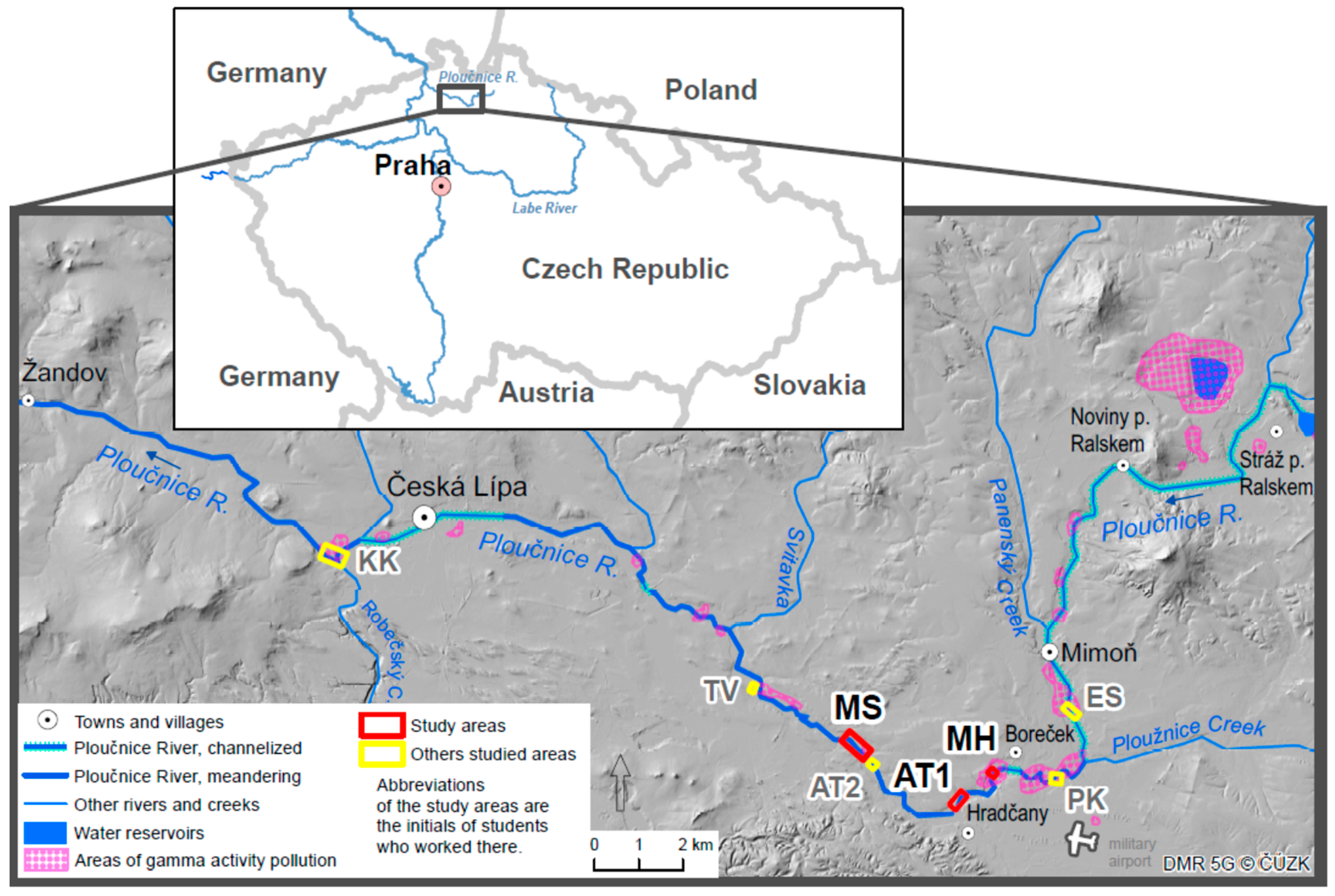
1.1. Study Areas
1.2. Pollution History of the Ploučnice River and Its Floodplain
2. Materials and Methods
2.1. GIS Data Collection and Processing
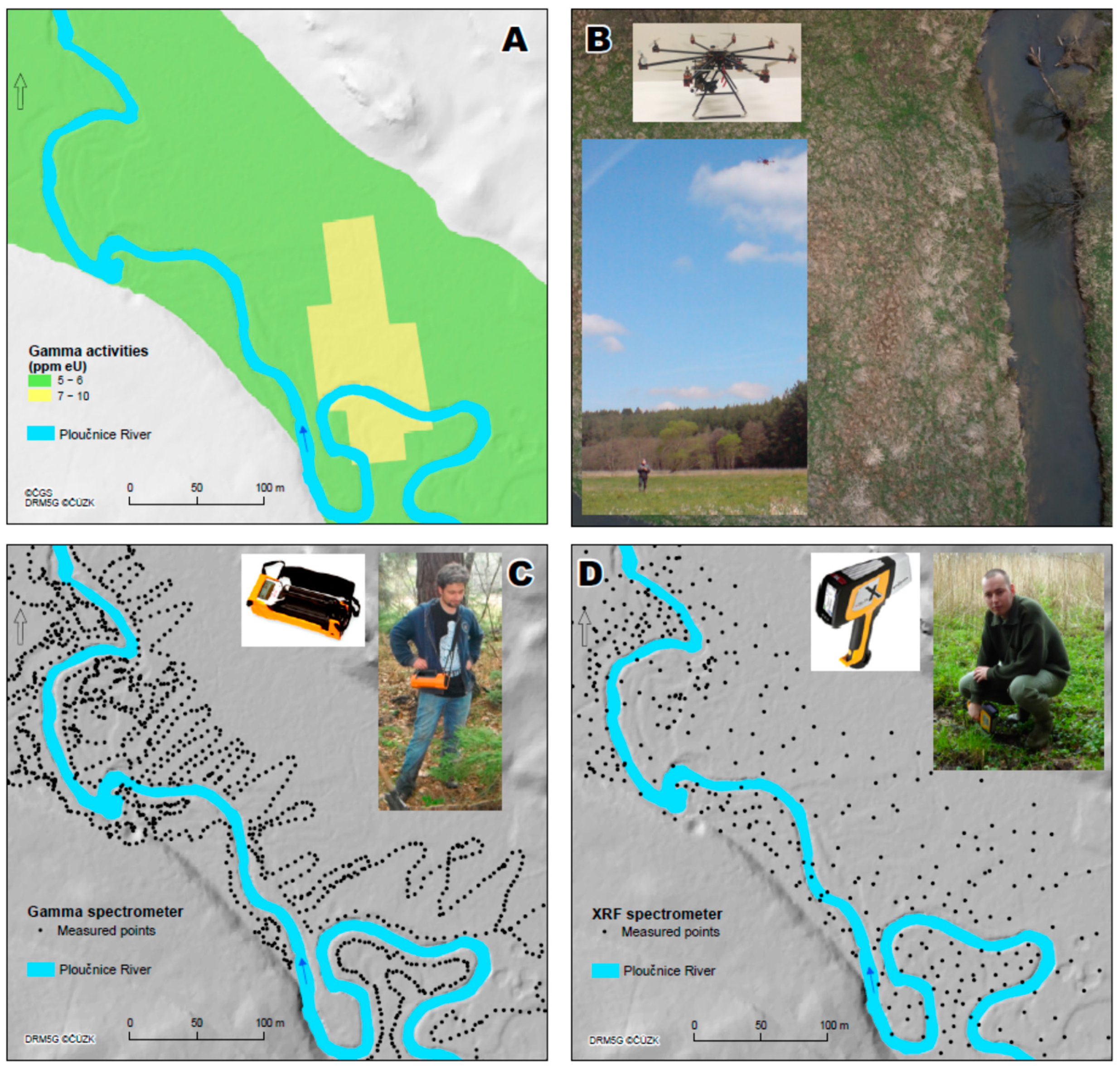
2.2. Pollution Mapping
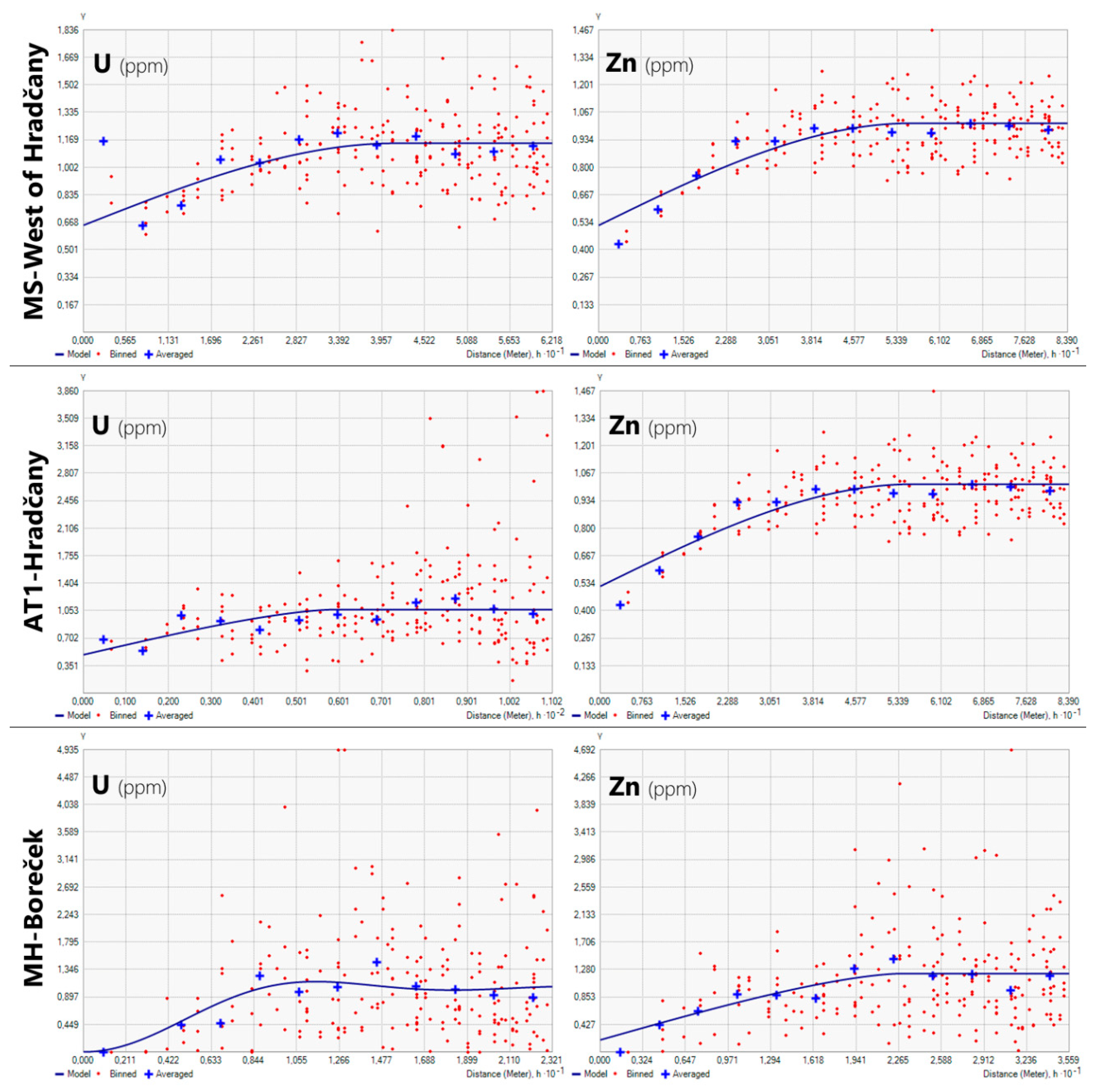
2.3. Geostatistical Analysis
3. Results
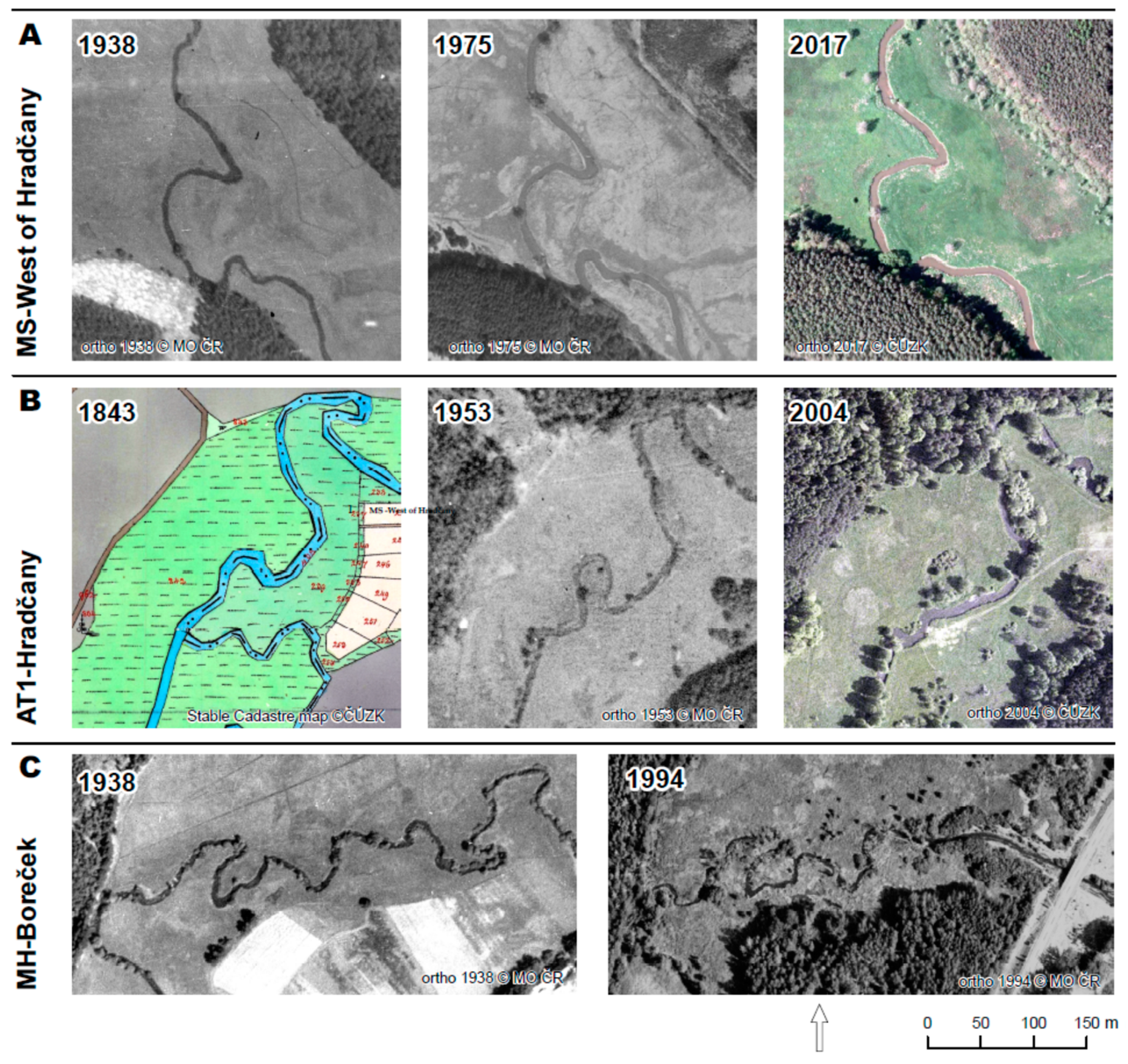
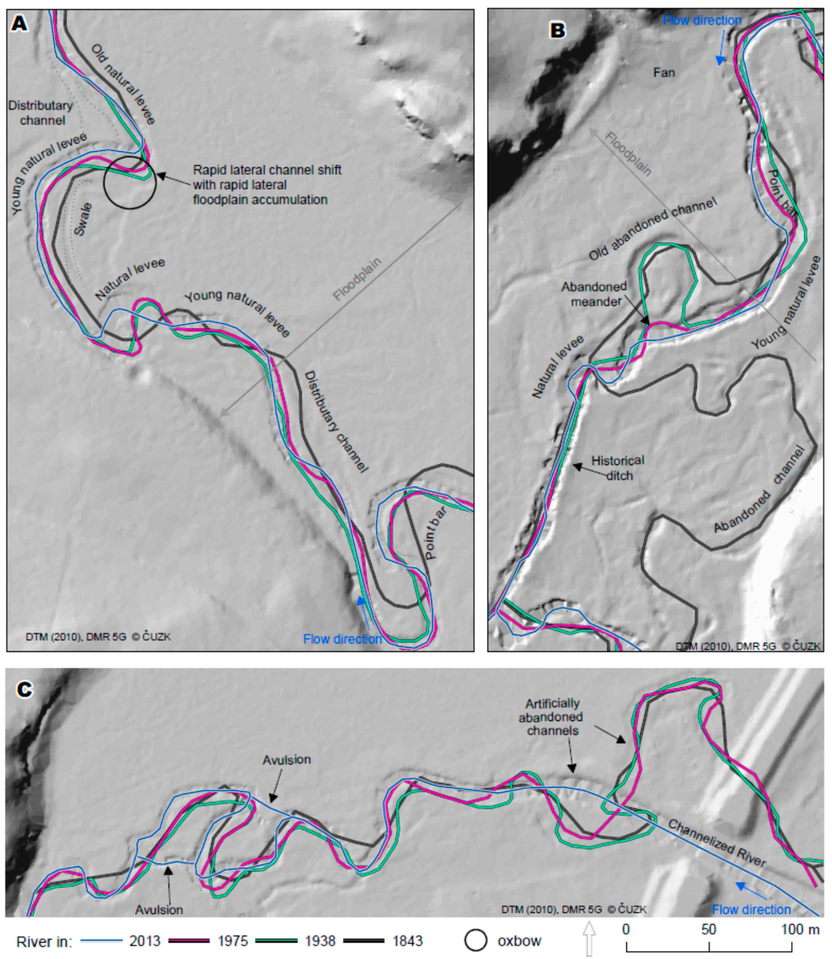
3.1. River Dynamics and Engineering
3.2. Pollution and Lithological Mapping
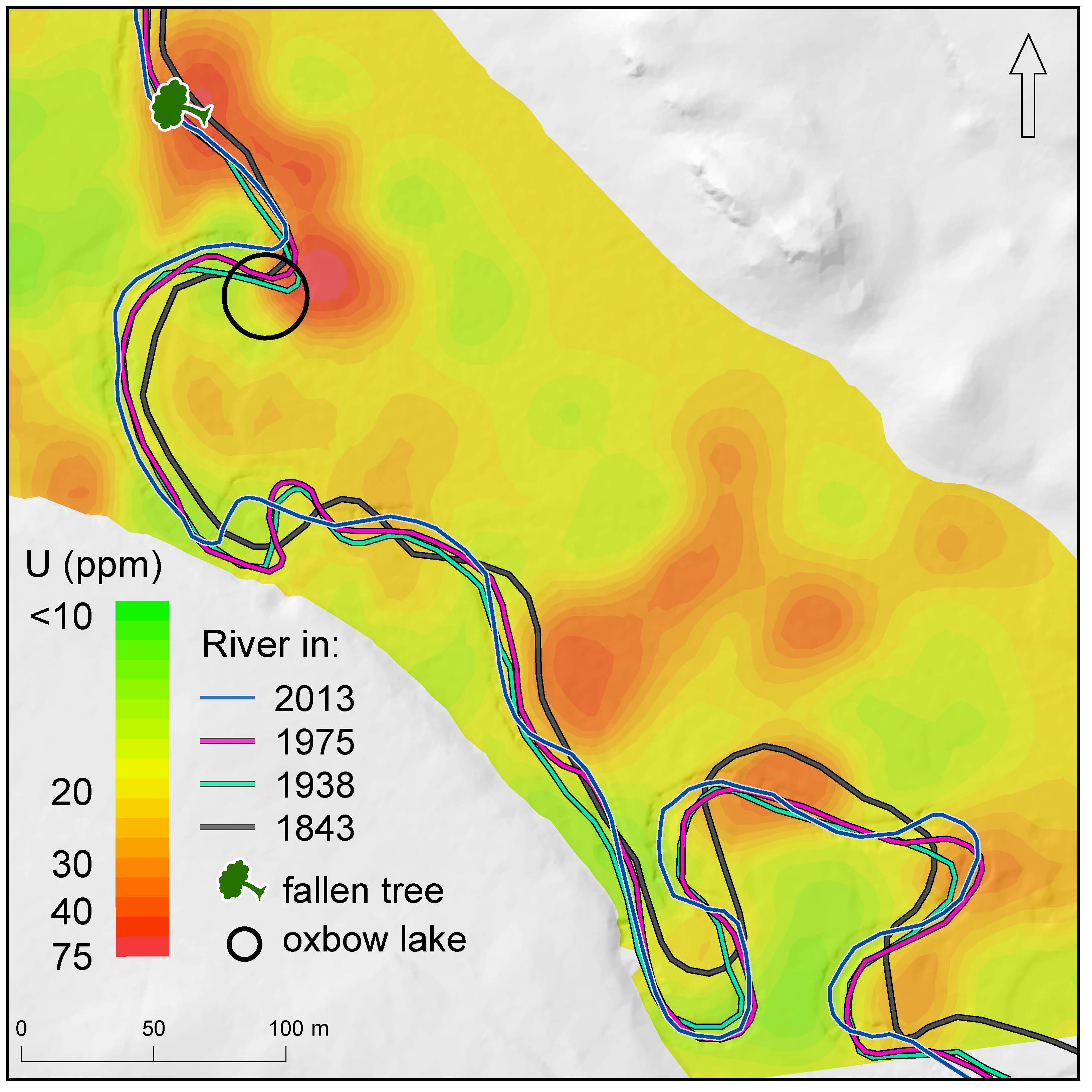
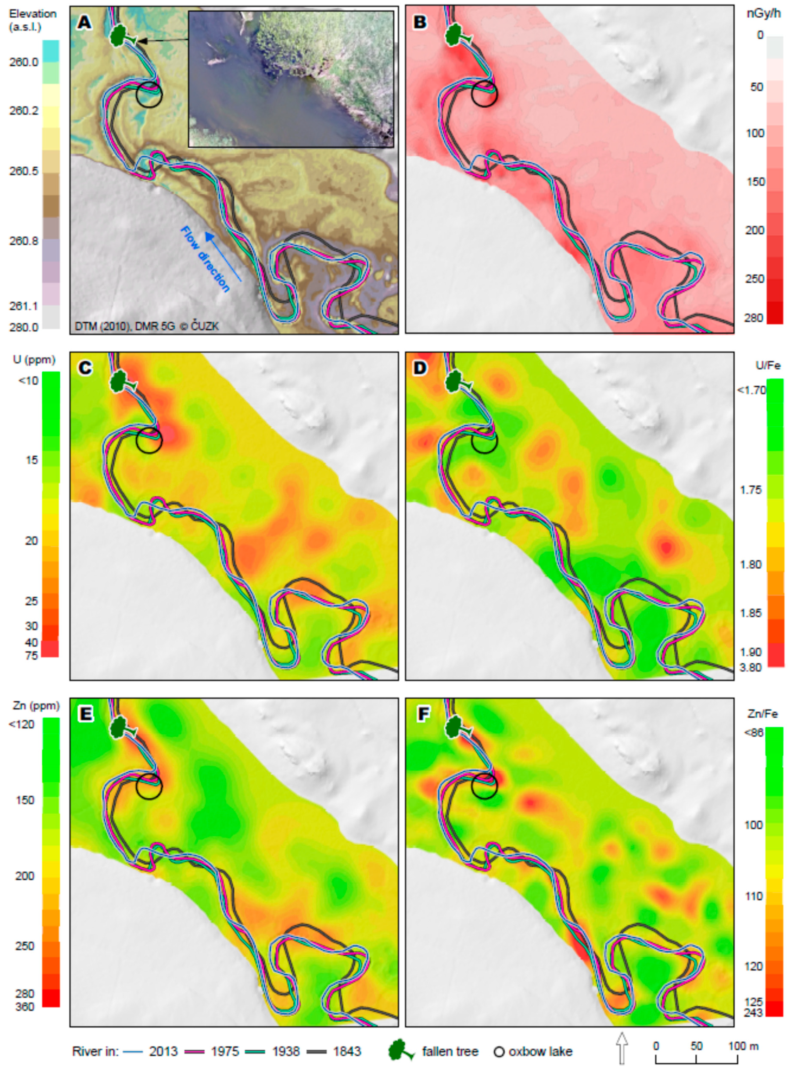
3.2.1. Pollution Mapping in the MS-West of Hradčany Study Area
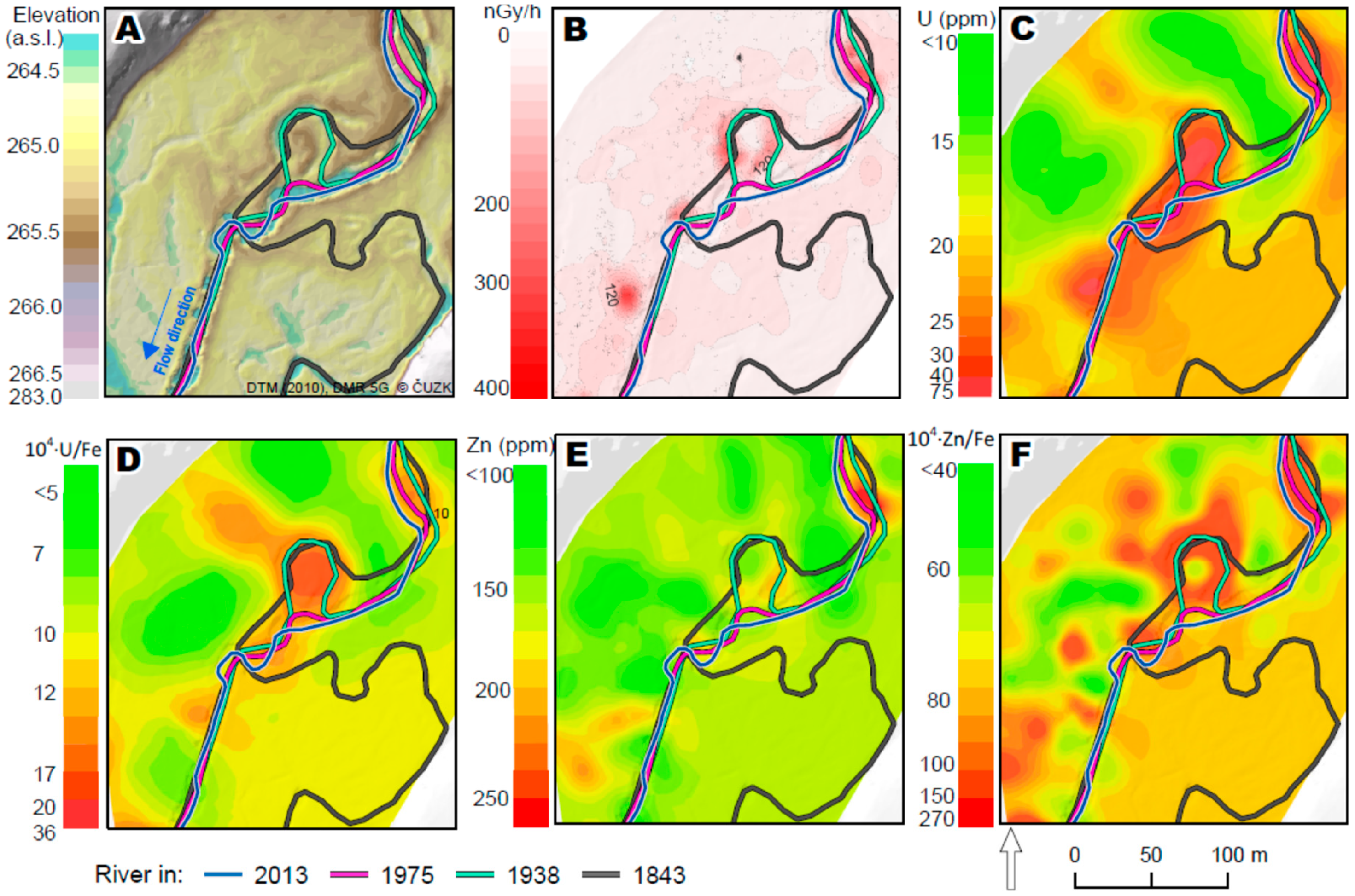
3.2.2. Pollution Mapping in the AT1–Hradčany Study Area
3.2.3. Pollution Mapping in the MH–Boreček Study Area
4. Discussion
- (1)
- sediments in abandoned meanders and laterally shifting channels that have evolved, i.e., were filled with sediment during the U-mining climax (1971–1989); these features can be identified with GIS analysis, in particular using old maps, aerial photographs and DTM;
- (2)
- other sediment traps in the floodplain, such as meander scars (more ancient channels not depicted in old maps [24]); and
- (3)
- certain young (recently built) levees; these locations can be identified with DTM on the external banks of meander bends and by “sedimentary facies mapping”, i.e., mapping sediment grain-size in the floodplain, because they exhibit lower Al/Si and/or higher Zr/Rb ratios in the Ploučnice River floodplain.
5. Conclusions
Author Contributions
Funding
Acknowledgments
Conflicts of Interest
References
- Miller, J.; Barr, R.; Grow, D.; Lechler, P.; Richardson, D.; Waltman, K.; Warwick, J. Effects of the 1997 flood on the transport and storage of sediment and mercury within the Carson River valley, west-central Nevada. J. Geol. 1999, 107, 313–327. [Google Scholar] [CrossRef]
- Ciszewski, D. Flood-related changes in heavy metal concentrations within sediments of the Biała Przemsza River. Geomorphology 2001, 40, 205–218. [Google Scholar] [CrossRef]
- Foulds, S.A.; Brewer, P.A.; Macklin, M.G.; Haresign, W.; Betson, R.E.; Rassner, S.M.E. Flood-related contamination in catchments affected by historical metal mining: An unexpected and emerging hazard of climate change. Sci. Total Environ. 2014, 476, 165–180. [Google Scholar] [CrossRef] [PubMed]
- Matys Grygar, T.; Elznicová, J.; Bábek, O.; Hošek, M.; Engel, Z.; Kiss, T. Obtaining isochrones from pollution signals in a fluvial sediment record: A case study in a uranium-polluted floodplain of the Ploučnice River, Czech Republic. Appl. Geochem. 2014, 48, 1–15. [Google Scholar] [CrossRef]
- Nováková, T.; Kotková, K.; Elznicová, J.; Strnad, L.; Engel, Z.; Matys Grygar, T. Pollutant dispersal and stability in a severely polluted floodplain: A case study in the Litavka River, Czech Republic. J. Geochem. Explor. 2015, 156, 131–144. [Google Scholar] [CrossRef]
- Wohl, E. Time and the rivers flowing: Fluvial geomorphology since 1960. Geomorphology 2014, 216, 263–282. [Google Scholar] [CrossRef]
- Houben, P. Geomorphological facies reconstruction of Late Quaternary alluvia by the application of fluvial architecture concepts. Geomorphology 2007, 86, 94–114. [Google Scholar] [CrossRef]
- Notebaert, B.; Houbrechts, G.; Verstraeten, G.; Broothaerts, N.; Haeckx, J.; Reynders, M.; Govers, G.; Petit, F.; Poesen, J. Fluvial architecture of Belgian river systems in contrasting environments: Implications for reconstructing the sedimentation history. Neth. J. Geosci. 2011, 90, 31–50. [Google Scholar] [CrossRef]
- Matys Grygar, T.; Elznicová, J.; Tůmová, Š.; Faměra, M.; Balogh, M.; Kiss, T. Floodplain architecture of an actively meandering river (the Ploučnice River, the Czech Republic) as revealed by the distribution of pollution and electrical resistivity tomography. Geomorphology 2016, 254, 41–56. [Google Scholar] [CrossRef]
- Faměra, M.; Kotková, K.; Tůmová, Š.; Elznicová, J.; Matys Grygar, T. Pollution distribution in floodplain structure visualised by electrical resistivity imaging in the floodplain of the Litavka River, the Czech Republic. CATENA 2018, 165, 157–172. [Google Scholar] [CrossRef]
- Matys Grygar, T.; Nováková, T.; Bábek, O.; Elznicová, J.; Vadinová, N. Robust assessment of moderate heavy metal contamination levels in floodplain sediments: A case study on the Jizera River, Czech Republic. Sci. Total Environ. 2013, 452, 233–245. [Google Scholar] [CrossRef]
- Stacke, V.; Pánek, T.; Sedláček, J. Late Holocene evolution of the Bečva River floodplain (Outer Western Carpathians, Czech Republic). Geomorphology 2014, 206, 440–451. [Google Scholar] [CrossRef]
- Marks, K.; Bates, P. Integration of high-resolution topographic data with floodplain flow models. Hydrol. Process. 2000, 14, 2109–2122. [Google Scholar] [CrossRef]
- Gałuszka, A.; Migaszewski, Z.; Namieśnik, J. Moving your laboratories to the field—Advantages and limitations of the use of field portable instruments in environmental sample analysis. Environ. Res. 2015, 140, 593–603. [Google Scholar] [CrossRef] [PubMed]
- Hürkamp, K.; Raab, T.; Voelkel, J. Two and three-dimensional quantification of lead contamination in alluvial soils of a historic mining area using field portable X-ray fluorescence (FPXRF) analysis. Geomorphology 2009, 110, 28–36. [Google Scholar] [CrossRef]
- Weindorf, D.C.; Zhu, Y.; Chakraborty, S.; Bakr, N.; Huang, B. Use of portable X-ray fluorescence spectrometry for environmental quality assessment of peri-urban agriculture. Environ. Monit. Assess. 2012, 184, 217–227. [Google Scholar] [CrossRef] [PubMed]
- Parsons, C.; Grabulosa, E.M.; Pili, E.; Floor, G.H.; Roman-Ross, G.; Charlet, L. Quantification of trace arsenic in soils by field-portable X-ray fluorescence spectrometry: Considerations for sample preparation and measurement conditions. J. Hazard. Mater. 2013, 262, 1213–1222. [Google Scholar] [CrossRef] [PubMed]
- Brumbaugh, W.G.; Tillitt, D.E.; May, T.W.; Javzan, Ch.; Komov, V.T. Environmental survey in the Tuul and Orkhon River basins of north-central Mongolia, 2010: Metals and other elements in streambed sediment and floodplain soil. Environ. Monit. Assess. 2013, 185, 8991–9008. [Google Scholar] [CrossRef]
- Kühn, J. Distribuce Uranu a Vybraných Těžkých Kovů v Sedimentech údolní Nivy Ploučnice (Distribution of Uranium and Selected Heavy Metals in Sediments of the Floodplain of the Ploučnice River). Ph.D. Thesis, Faculty of Science Charles University, Prague, Czech Republic, 1996. [Google Scholar]
- Martin, P.G.; Payton, O.D.; Fordoulis, J.S.; Richards, D.A.; Scott, T.B. The use of unmanned aerial systems for the mapping of legacy uranium mines. J. Environ. Radioact. 2015, 143, 135–140. [Google Scholar] [CrossRef] [Green Version]
- Hošek, M. Kontaminace nivy Ploučnice Těžkými Kovy ve Vztahu k Její Architektuře (Pollution of Ploučnice Floodplain by Heavy Metals in Relation to Its Architecture). Master’s Thesis, Faculty of Science Charles University, Prague, Czech Republic, 2015. [Google Scholar]
- Slabá, E.; Matys Grygar, T.; Elznicová, J. Posouzení navržených revitalizačních opatření řeky Ploučnice u Mimoně z hlediska remobilizace historické kontaminace. (Evaluation of proposed revitalization of the river Ploučnice close to Mimoň in terms of remobilization of historical contamination). In Proceedings of the Krajinné inženýrství 2015. Provoz a údržba staveb krajinného inženýrství 2015, Prague, Czech Republic, 17 September 2015; Česká společnost krajinných inženýrů: Praha, Czech Republic, 2015; pp. 105–120, ISBN 978-80-87384-07-7. [Google Scholar]
- Elznicová, J.; Plotnárek, L. Reconstruction of historical landscape from aerial photographs for river development assessment. In Proceedings of the 14th SGEM GeoConference on Informatics, Geoinformatics and Remote Sensing, SGEM2014 Conference Proceedings, Albena, Bulgaria, 19–25 June 2014; Volume 3, pp. 269–2704, ISBN 978-619-7105-12-4. [Google Scholar] [CrossRef]
- Hošek, M.; Matys Grygar, T.; Elznicová, J.; Faměra, M.; Popelka, J.; Matkovič, J.; Kiss, T. Geochemical mapping in polluted floodplains using in situ X-ray fluorescence analysis, geophysical imaging, and statistics: Surprising complexity of floodplain pollution hotspot. CATENA 2018, 171, 632–644. [Google Scholar] [CrossRef]
- Elznicová, J.; Hrubešová, D. Spatiotemporal changes of the Ploučnice River for the explanation of pollution distribution in the floodplain. In Proceedings of the SGEM 2017 Conference on 17th International Multidisciplinary Scientific GeoConference SGEM 2017, Albena, Bulgaria, 29 June–5 July 2017; STEF92 Technology: Sofia, Bulgaria, 2017; Volume 17, pp. 665–672. [Google Scholar] [CrossRef]
- Slabá, E. Posouzení Navržených Revitalizačních Opatření řeky Ploučnice u Mimoně z Hlediska Remobilizace Historické Kontaminace (Evaluation of Proposed Revitalization of the river Ploučnice Close to Mimoň in Terms of Remobilization of Historical Contamination). Master’s Thesis, J.E. Purkyně University in Ústí nad Labem, Ústí nad Labem, Czech Republic, 2015. [Google Scholar]
- Sikora, M. Zhodnocení Vývoje Radioaktivního Znečistění Toku a údolní Nivy Ploučnice (The Evaluation of Radioactive Contamination of the Ploučnice River and Floodplain). Master’s Thesis, J.E. Purkyně University in Ústí nad Labem, Ústí nad Labem, Czech Republic, 2016. [Google Scholar]
- Váchová, T. Využití Geostatických Metod Při Mapování Znečištění v Nivě řeky Ploučnice (Application of Geostatistical Methods for Mapping Pollution in the River Floodplain Ploucnice). Master’s Thesis, J.E. Purkyně University in Ústí nad Labem, Ústí nad Labem, Czech Republic, 2017. [Google Scholar]
- Elznicová, J.; Matys Grygar, T.; Sikora, M.; Popelka, J.; Hošek, M.; Novák, P. Threat of pollution hotspots reworking in river systems: Example of the Ploučnice River (Czech Republic). In Proceedings of the GIS for Safety & Security Management, GIS Ostrava 2018, Ostrava, Czech Republic, 21–23 March 2018; Ivan, I., Caha, J., Burian, J., Eds.; VŠB Technical University of Ostrava: Ostrava, Czech Republic, 2018; pp. 159–176, ISBN 978-80-248-4235-6. [Google Scholar]
- Klimešová, K. Mapování znečištění nivy řeky Ploučnice (Floodplain mapping of pollution of the river Ploučnice). Master’s Thesis, J.E. Purkyně University in Ústí nad Labem, Ústí nad Labem, Czech Republic, 2018. [Google Scholar]
- Tipanová, A. Transport Polutantů z Těžby a Zpracování Uranu říčním Systémem Ploučnice (Transport of Pollutants from Minig and Processing of Uranium in River System Ploučnice). Master’s Thesis, Department of Geology, Faculty of Science Palacký University, Olomouc, Czech Republic, 2016. [Google Scholar]
- Vitáček, Z.; Knauerová, M.; Kühn, P. Řeka Ploučnice a Příroda v Okolí (Ploučnice River and Nature around). Mikroregion Podralsko. Available online: http://www.podralsko.info/zelena-cyklomagistrala- ploucnice/informace-o-rece-ploucnice/ (accessed on 7 February 2018).
- Novák, M.; Emmanuel, S.; Vile, M.A.; Erel, Y.; Véron, A.; Pačes, T.; Wieder, R.K.; Vaněček, M.; Štěpánová, M.; Břízová, E.; et al. Origin of lead in eight Central European peat bogs determined from isotope ratios, strengths, and operation times of regional pollution sources. Environ. Sci. Technol. 2003, 37, 437–445. [Google Scholar] [CrossRef] [PubMed]
- Matys Grygar, T.; Sedláček, J.; Bábek, O.; Nováková, T.; Strnad, L.; Mihaljevič, M. Regional contamination of Moravia (south-eastern Czech Republic): Temporal shift of Pb and Zn loading in fluvial sediments. Water Air Soil Pollut. 2012, 223, 739–753. [Google Scholar] [CrossRef]
- Majerová, L.; Matys Grygar, T.; Elznicová, J.; Strnad, L. The Differentiation between Point and Diffuse Industrial Pollution of the Floodplain of the Ploucnice River, Czech Republic. Water Air Soil Pollut. 2013, 224, 1688. [Google Scholar] [CrossRef]
- Hrdoušek, F. Těžké kovy v sedimentech Panenského potoka a středního toku Ploučnice (Heavy metals in sediments of Panenský Creek and middle reach of Ploučnice). Master’s Thesis, Faculty of Science Charles University, Prague, Czech Republic, 2005. [Google Scholar]
- Kühn, P. Radioaktivní znečištění údolní nivy Ploučnice v bývalém VVP Ralsko (Radioactive pollution of the floodplain of the Ploučnice in former military area Ralsko). Available online: http://www.strazpr.cz/radioaktivni-znecisteni-v-severozapadni-casti-byvaleho-vvp-ralsko/d-3708 (accessed on 31 December 2018).
- Kafka, J. Rudné a Uranové Hornictví České Republiky (Ore and Uranium Mining in the Czech Republic); Anagram: Ostrava, Czech Republic, 2003; ISBN 80-86331-67-9. [Google Scholar]
- Slezák, J. Historie těžby uranu v oblasti Stráže pod Ralskem v severočeské křídě a hydrogeologie (History of uranium production in the area of Stráž pod Ralskem (the North Bohemian Cretaceous basin) and hydrogeology). Sbor. Geol. Věd. Hydrogeol. inž. Geol. 2000, 21, 5–36. [Google Scholar]
- Hanslík, E. Vliv těžby Uranových Rud na vývoj Kontaminace Hydrosféry Ploučnice v Období 1966–2000 (Impact of Uranium Ore Mining on Course of Pollution of Ploučnice Hydrosphere in Period of 1966–2000); Výzkumný ústav vodohospodářský T.G.: Prague, Czech Republic, 2002. [Google Scholar]
- Gnojek, I.; Dědáček, K.; Zabadal, S.; Sedlák, J. Letecké geofyzikální mapování radioaktivních zátěží Liberecka (Aerial Geophysical Mapping of Radioactive Loads of the Liberec Area); Final Report; Geofond Praha (The archive of the Czech Geological Survey): Prague, Czech Republic, 2005. [Google Scholar]
- Kolář, J. Distribuce Vybraných Těžkých Kovů v Sedimentech Horního Toku Ploučnice (Distribution of Selected Heavy Metals in Sediments of Upper Reach of Ploučnice). Master’s Thesis, Faculty of Science Charles University, Prague, Czech Republic, 2004. [Google Scholar]
- Digitální model reliéfu České republiky 5. generace (DMR 5G) (Digital Terrain Model of the Czech Republic 5th Generation). Available online: https://geoportal.cuzk.cz/(S(npqw1dtiaknauys50u2ty42r))/ Default.aspx?lng=EN&mode=TextMeta&side=vyskopis&metadataID=CZ-CUZK-DMR5G-V&head_tab=sekce-02-gp&menu=302 (accessed on 31 December 2018).
- Dilts, T.E. Stream Gradient and Sinuosity Toolbox for ArcGIS 10.1. University of Nevada Reno, 2015. Available online: http://www.arcgis.com/home/item.html?id=c8eb4ce1384e45258ccba1b33cd4e3cb (accessed on 31 December 2018).
- Grygar, T.; Světlík, I.; Lisá, L.; Koptíková, L.; Bajer, A.; Wray, D.S.; Ettler, V.; Mihaljevič, M.; Nováková, T.; Koubová, M.; et al. Geochemical tools for the stratigraphic correlation of floodplain deposits of the Morava River in Strážnické Pomoraví, Czech Republic from the last millennium. CATENA 2010, 80, 106–121. [Google Scholar] [CrossRef]
- Bouchez, J.; Gaillardet, J.; France-Lanord, C.; Maurice, L.; Dutra-Maia, P. Grain size control of river suspended sediment geochemistry: Clues from Amazon River depth profiles. Geochem. Geophys. Geosyst. 2011, 12, 1525–2027. [Google Scholar] [CrossRef]
- Bábek, O.; Matys Grygar, T.; Faměra, M.; Hron, K.; Nováková, T.; Sedláček, J. Geochemical background in polluted river sediments: How to separate the effects of sediment provenance and grain size with statistical rigour? CATENA 2015, 135, 240–253. [Google Scholar] [CrossRef]
- Dypvik, H.; Harris, N.B. Geochemical facies analysis of fine-grained siliciclastics using Th/U, Zr/Rb and (Zr+Rb)/Sr ratios. Chem. Geol. 2001, 181, 131–146. [Google Scholar] [CrossRef]
- Jones, A.F.; Macklin, M.G.; Brewer, P.A. A geochemical record of flooding on the upper River Severn, UK, during the last 3750 years. Geomorphology 2012, 179, 89–105. [Google Scholar] [CrossRef]
- Vijver, M.G.; Spijker, J.; Vink, J.P.M.; Posthuma, L. Determining metal origins and availability in fluvial deposits by analysis of geochemical baselines and solid-solution partitioning measurements and modelling. Environ. Pollut. 2008, 156, 832–839. [Google Scholar] [CrossRef]
- Jiang, J.-B.; Wang, J.; Liu, S.-Q.; Lin, C.-Y.; He, M.-C.; Li, X.-T. Background, baseline, normalization, and contamination of heavy metals in the Liao River Watershed sediments of China. J. Asian Earth Sci. 2013, 73, 87–94. [Google Scholar] [CrossRef]
- Guo, Y.-Q.; Huang, C.-C.; Pang, J.L.; Zha, X.-C.; Li, X.P.; Zhang, Y.Z. Concentration of heavy metals in the modern flood slackwater deposits along the upper Hanjiang River valley, China. CATENA 2014, 116, 123–131. [Google Scholar] [CrossRef]
- Wang, J.; Liu, G.-J.; Lu, L.-L.; Zhang, J.-M.; Liu, H.-Q. Geochemical normalization and assessment of heavy metals (Cu, Pb, Zn, and Ni) in sediments from the Huaihe River, Anhui, China. CATENA 2015, 129, 30–38. [Google Scholar] [CrossRef]
- Matys Grygar, T.; Popelka, J. Revisiting geochemical methods of distinguishing natural concentrations and pollution b risk elements in fluvial sediments. J. Geochem. Explor. 2016, 170, 39–57. [Google Scholar] [CrossRef]
- Löwemark, L.; Chen, H.-F.; Yang, T.-N.; Kylander, M.; Yu, E.-F.; Hsu, Y.-W.; Lee, T.-Q.; Song, S.-R.; Jarvis, S. Normalizing XRF-scanner data: A cautionary note on the interpretation of high-resolution records from organic-rich lakes. J. Asian Earth Sci. 2011, 40, 1250–1256. [Google Scholar] [CrossRef]
- Oliver, M.A.; Webster, R. A tutorial guide to geostatistics: Computing and modelling variograms and kriging. CATENA 2014, 113, 56–69. [Google Scholar] [CrossRef]
- ESRI. ArcGIS Desktop: Release 10.6. Environmental Systems Research Institute, Redlands, 2018. Available online: http://desktop.arcgis.com/en/arcmap/latest/extensions/geostatistical-analyst/ what-is-geostatistics-.htm (accessed on 31 December 2018).
- Wackernagel, H. Multivariate Geostatistics: An Introduction with Applications; Springer: Berlin, Germany, 2003; p. 25. ISBN 978-3-662-05294-5. [Google Scholar]
- Li, J.; Heap, A.D. A Review of Spatial Interpolation Methods for Environmental Scientists; Record 2008/23; Geoscience Australia: Canberra, Australia, 2008; pp. 154–196. ISBN 978-1-921498-28-2.
- Burrough, P.A.; McDonnell, R.; McDonnell, R.A.; Lloyd, C.H.D. Principles of Geographical Information Systems; Oxford University Press: Oxford, UK, 2015; p. 174. ISBN 978-0-19-874284-5. [Google Scholar]
- Zuo, X.; Zhao, H.; Zhao, X.; Zhang, T.; Guo, Y.; Wang, S.; Drake, S. Spatial pattern and heterogeneity of soil properties in sand dunes under grazing and restoration in Horqin Sandy Land, Northern China. Soil Tillage Res. 2008, 99, 202–212. [Google Scholar] [CrossRef]
- Argyraki, A.; Ramsey, M.H.; Potts, P.J. Evaluation of Portable X-ray Fluorescence Instrumentation for in situ Measurements of Lead on Contaminated Land. Analyst 1997, 122, 743–749. [Google Scholar] [CrossRef] [Green Version]
- Weindorf, D.C.; Bakr, N.; Zhu, Y.; Mcwhirt, A.; Ping, C.L.; Michaelson, G.; Nelson, C.; Shook, K.; Nuss, S. Influence of Ice on Soil Elemental Characterization via Portable X-Ray Fluorescence Spectrometry. Pedosphere 2014, 24, 1–12. [Google Scholar] [CrossRef]
- Matys Grygar, T. Letter to Editor re Pavlović et al. (2015). Sci. Total Environ. 2016, 547, 482–483. [Google Scholar] [CrossRef]
- Ciszewski, D. Channel processes as a factor controlling accumulation of heavy metals in river bottom sediments: Consequences for pollution monitoring (Upper Silesia, Poland). Environ. Geol. 1998, 36, 45–54. [Google Scholar] [CrossRef]
- Navrátil, T.; Rohovec, J.; Žák, K. Floodplain sediments of the 2002 catastrophic flood at the Vltava (Moldau) River and its tributaries: Mineralogy, chemical composition, and post-sedimentary evolution. Environ. Geol. 2008, 56, 399–412. [Google Scholar] [CrossRef]
- Bábek, O.; Faměra, M.; Hilscherová, K.; Kalvoda, J.; Dobrovolný, P.; Sedláček, J. Geochemical traces of flood layers in the fluvial sedimentary archive; implications for contamination history analyses. CATENA 2011, 87, 281–290. [Google Scholar] [CrossRef]
- Dhivert, E.; Grosbois, C.; Rodrigues, S.; Desmet, M. Influence of fluvial environments on sediment archiving processes and temporal pollutant dynamics (Upper Loire River, France). Sci. Total Environ. 2015, 505, 121–136. [Google Scholar] [CrossRef] [PubMed]


| MS-West of Hradčany | ||||||
| XRF Value | Estimated Mean | Variogram Function | Nugget | Nugget-to-Sill Ratio (%) | Major Range | RMSPE |
| U | 0.002 | Spherical | 0.650 | 57 | 41.455 | 0.903 |
| U/Fe | 0.000 | Circular | 0.864 | 92 | 41.316 | 1.068 |
| Zn | 0.019 | Spherical | 0.519 | 51 | 55.936 | 1.035 |
| Zn/Fe | 0.011 | Circular | 0.761 | 76 | 27.933 | 1.004 |
| Al/Si | 0.303 | J-Bessel | 0.381 | 38 | 113.408 | 0.977 |
| Zr/Rb | 4.903 | Circular | 0.237 | 27 | 58.651 | 1.065 |
| AT1-Hradčany | ||||||
| XRF Value | Estimated Mean | Variogram Function | Nugget | Nugget-to-Sill Ratio (%) | Major Range | RMSPE |
| U | 0.002 | Circular | 0.490 | 46 | 58.249 | 1.007 |
| U/Fe | 0.001 | Circular | 0.469 | 45 | 51.421 | 0.915 |
| Zn | 0.016 | Circular | 0.578 | 55 | 26.673 | 0.913 |
| Zn/Fe | 0.008 | Spherical | 0.370 | 39 | 26.456 | 0.941 |
| Al/Si | 0.210 | Spherical | 0.377 | 39 | 50.921 | 0.950 |
| Zr/Rb | 5.128 | J-Bessel | 0.405 | 41 | 83.895 | 0.894 |
| MH-Boreček | ||||||
| XRF Value | Estimated Mean | Variogram Function | Nugget | Nugget-to-Sill Ratio (%) | Major Range | RMSPE |
| U | 0.003 | J-Bessel | 0 | 0 | 15.472 | 1.020 |
| U/Fe | 0.001 | Circular | 0 | 0 | 12.495 | 0.958 |
| Zn | 0.040 | Circular | 0.186 | 15 | 22.645 | 1.007 |
| Zn/Fe | 0.016 | Exponential | 0 | 0 | 12.739 | 1.116 |
| Al/Si | 0.203 | Circular | 0.001 | 0 | 73.179 | 1.002 |
| Zr/Rb | 4.866 | J-Bessel | 0.162 | 17 | 43.458 | 0.982 |
| Study Area | Hotspot Position | Methods Used | References |
|---|---|---|---|
| ES-South of Mimoň | Former depression in floodplain (meander scar?) | GIS, gamma, XRF, laboratory XRF, geostatistical analysis | [22,26] |
| PK-Boreček | Abandoned channel | AAS, gamma | [19] |
| MH-Boreček | Former depression in floodplain (old, shallow flood channel) | GIS, XRF, laboratory XRF, gamma, ERT, DEMP, OSL, geostatistics | [9,21,24,27] This work |
| AT1-Hradčany | Meander abandoned during U-mining | GIS, gamma, ERT, XRF, laboratory XRF, geostatistics | [9,27,31] This work |
| AT2-West of Hradčany | Meander-starting to cut-off | GIS, ERT, laboratory XRF | [9,31] |
| MS-West of Hradčany | Channel bars and natural levees | GIS, XRF, gamma, and drone maps, geostatistical analysis | [27,29] This work |
| TV-Veselí | Secondary river channel | GIS, gamma, XRF, laboratory XRF, geostatistical analysis | [28] |
| KK-by Česká Lípa | Depression in floodplain (shallow flood channel) | GIS, gamma, DEMP, XRF, laboratory XRF, geostatistical analysis | [30] |
© 2019 by the authors. Licensee MDPI, Basel, Switzerland. This article is an open access article distributed under the terms and conditions of the Creative Commons Attribution (CC BY) license (http://creativecommons.org/licenses/by/4.0/).
Share and Cite
Elznicová, J.; Matys Grygar, T.; Popelka, J.; Sikora, M.; Novák, P.; Hošek, M. Threat of Pollution Hotspots Reworking in River Systems: Case Study of the Ploučnice River (Czech Republic). ISPRS Int. J. Geo-Inf. 2019, 8, 37. https://0-doi-org.brum.beds.ac.uk/10.3390/ijgi8010037
Elznicová J, Matys Grygar T, Popelka J, Sikora M, Novák P, Hošek M. Threat of Pollution Hotspots Reworking in River Systems: Case Study of the Ploučnice River (Czech Republic). ISPRS International Journal of Geo-Information. 2019; 8(1):37. https://0-doi-org.brum.beds.ac.uk/10.3390/ijgi8010037
Chicago/Turabian StyleElznicová, Jitka, Tomáš Matys Grygar, Jan Popelka, Martin Sikora, Petr Novák, and Michal Hošek. 2019. "Threat of Pollution Hotspots Reworking in River Systems: Case Study of the Ploučnice River (Czech Republic)" ISPRS International Journal of Geo-Information 8, no. 1: 37. https://0-doi-org.brum.beds.ac.uk/10.3390/ijgi8010037