A Comparative Assessment of Geostatistical, Machine Learning, and Hybrid Approaches for Mapping Topsoil Organic Carbon Content

 ,
, 


Abstract
:
1. Introduction
2. Materials and Methods
2.1. Materials
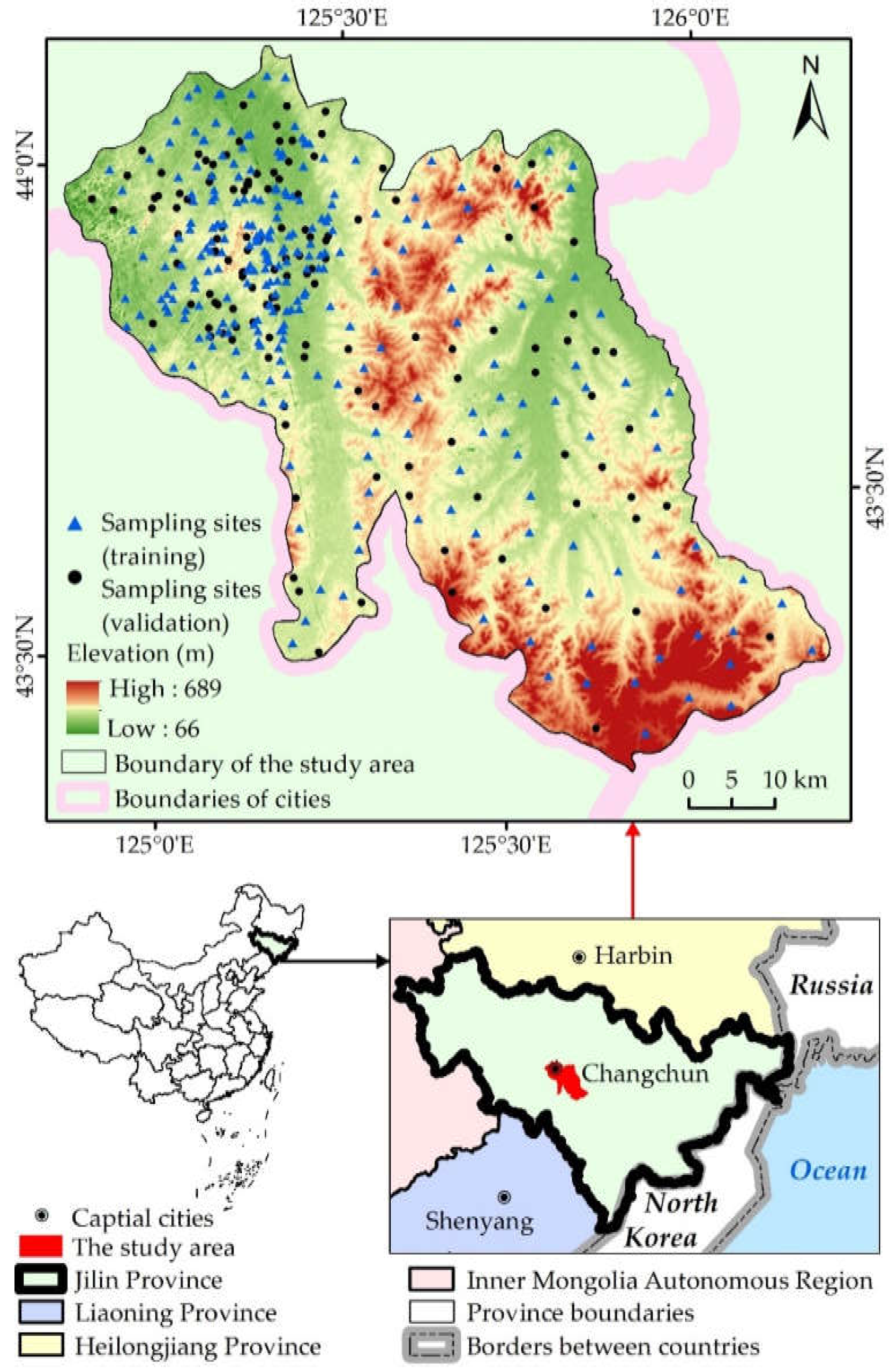
2.1.1. Study Area
2.1.2. Soil Observations
2.1.3. Environmental Variables
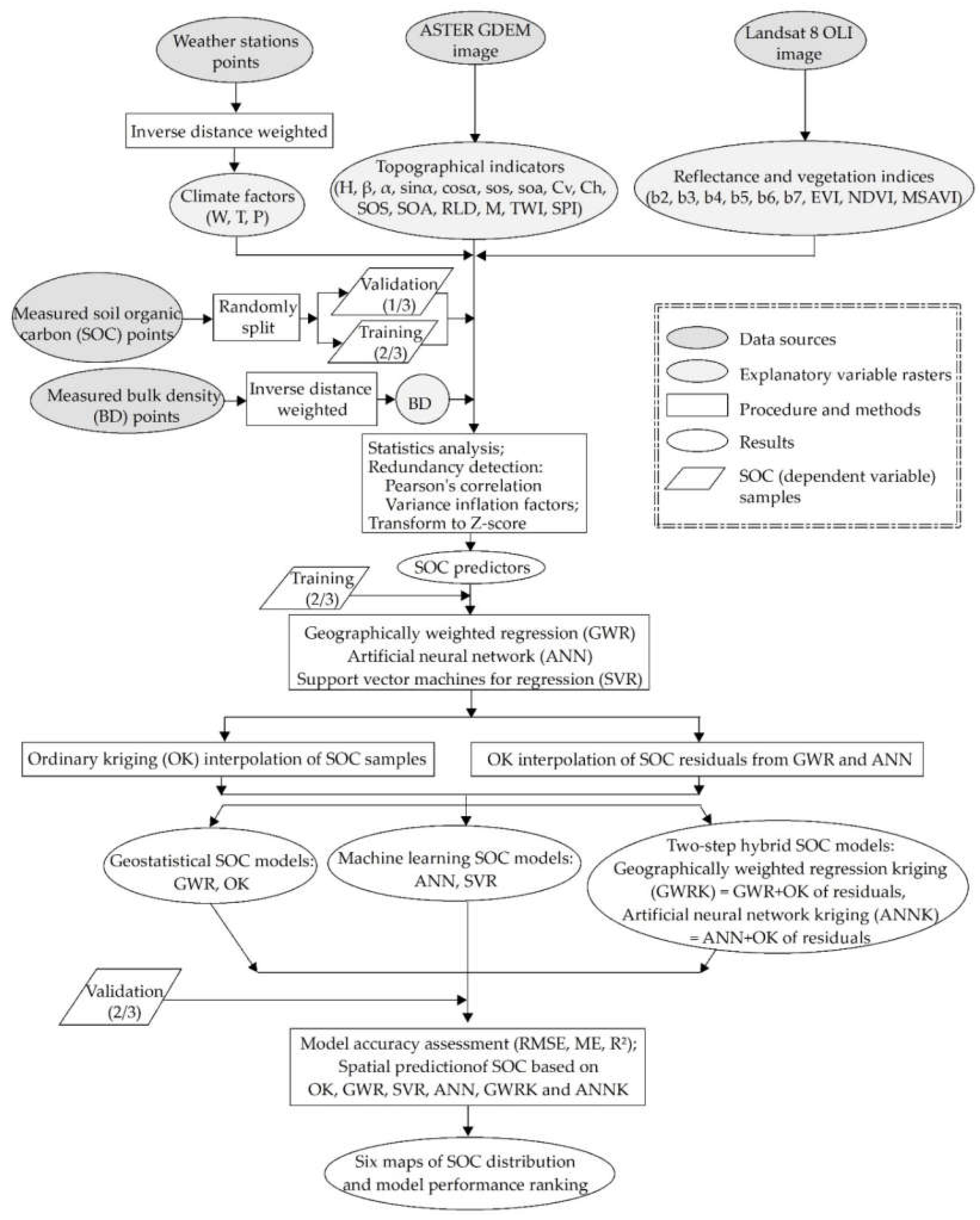
2.2. Modeling and Prediction
2.2.1. Statistical Analysis
2.2.2. Geostatistical Models
2.2.3. Machine Learning Methods
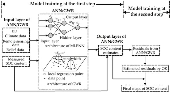
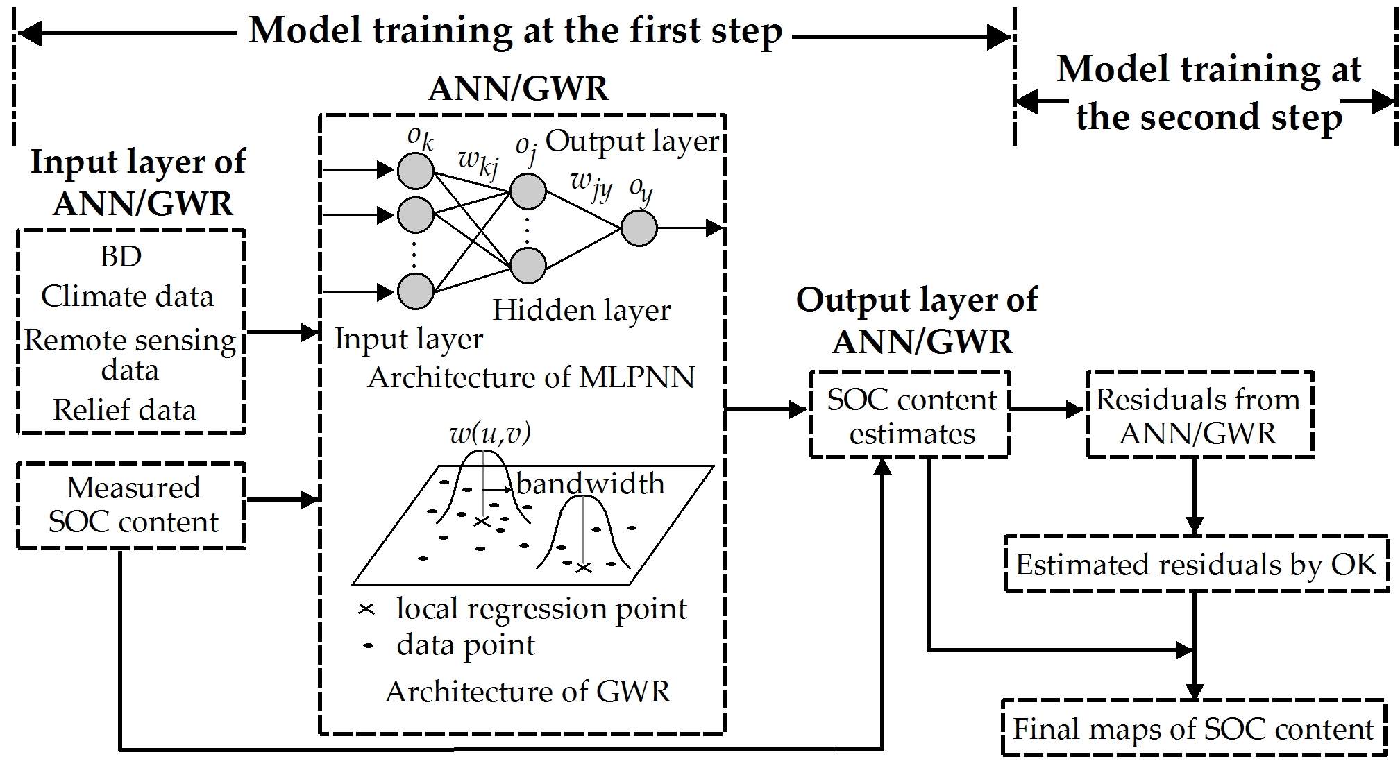
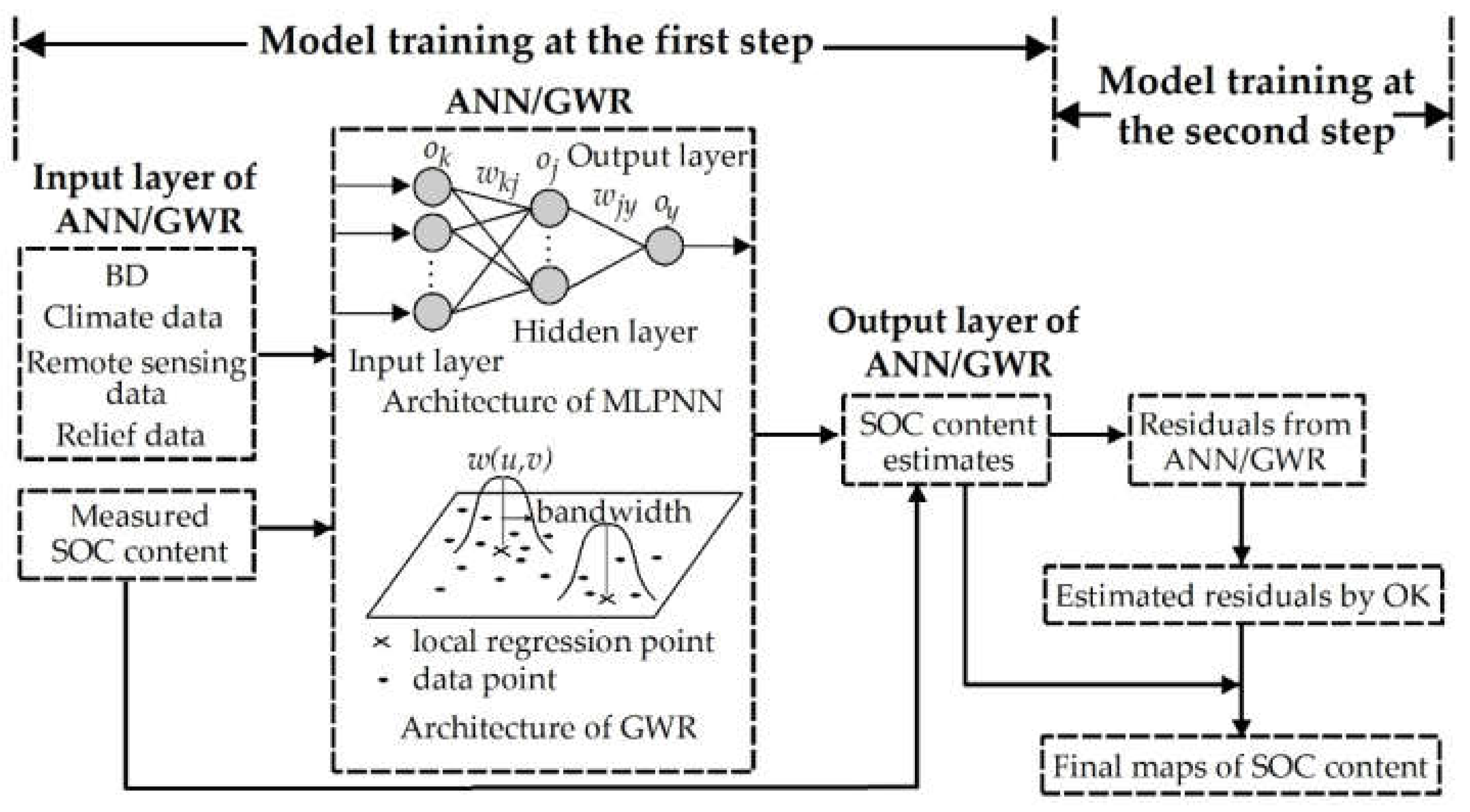
2.2.4. Two-Step Hybrid Approaches
2.2.5. Model Testing and Comparison
3. Results
3.1. Statistics Analysis
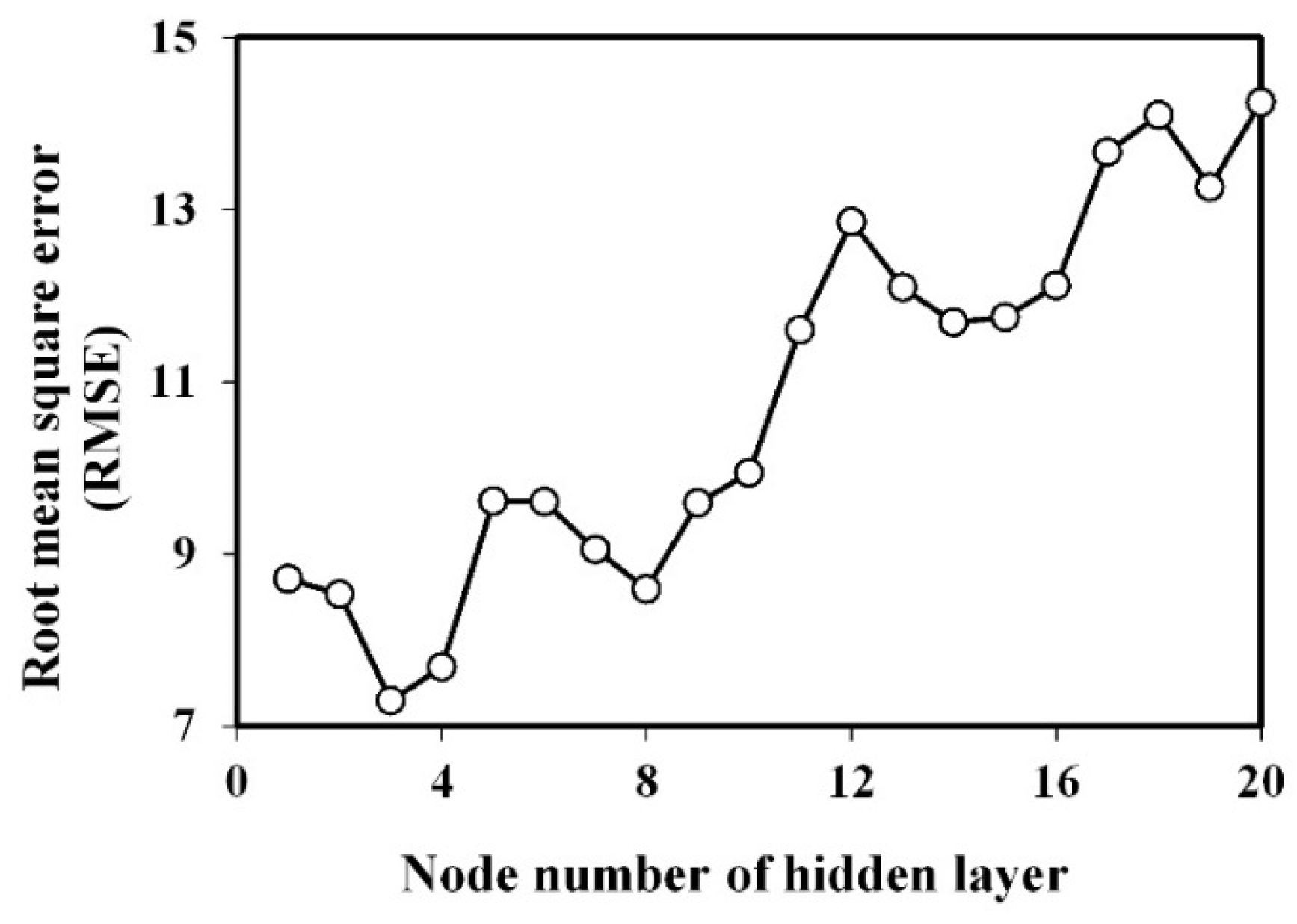
3.2. Models Training of GWR, SVR and ANN
3.3. OK, GWRK and ANNK Training and Six Models Validation
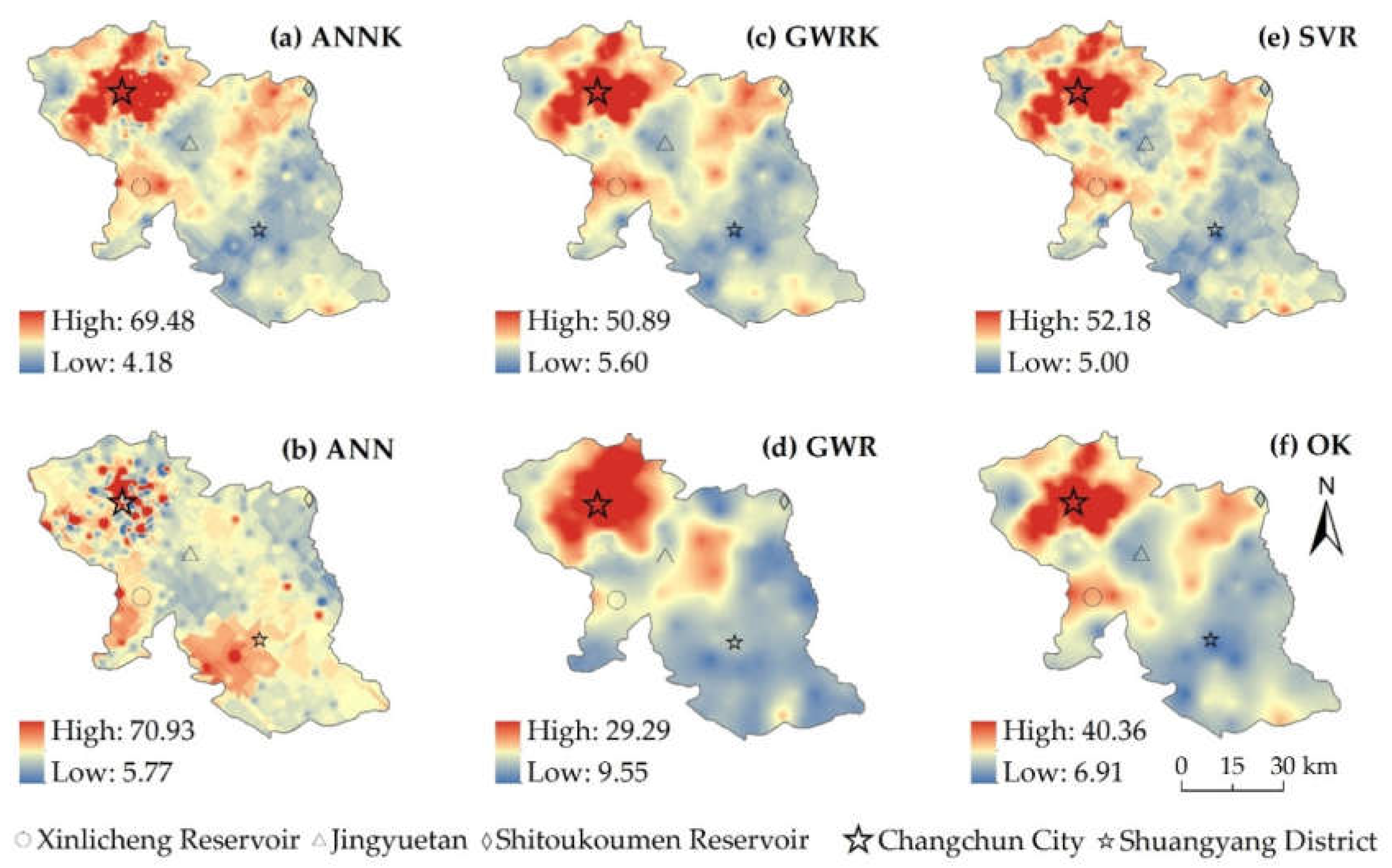
3.4. Spatial Prediction and Mapping of SOC Content
4. Discussion
4.1. Comparison between Intra-Classes of Three DSM Techniques
4.2. Comparison among Geostatistical, ML and Hybrid Techniques
5. Conclusions
Author Contributions
Funding
Acknowledgments
Conflicts of Interest
References
- Jobbágy, E.G.; Jackson, R.B. The vertical distribution of soil organic C and its relation to climate and vegetation. Ecol. Appl. 2000, 10, 423–436. [Google Scholar] [CrossRef]
- Stockmann, U.; Adams, M.A.; Crawford, J.W.; Field, D.J.; Henakaarchchi, N.; Jenkins, M.; Minasny, B.; McBratney, A.B.; de Courcelles, V.D.; Singh, K.; et al. The knowns, known unknowns and unknowns of sequestration of soil organic carbon. Agric. Ecosyst. Environ. 2013, 164, 80–99. [Google Scholar] [CrossRef]
- Davidson, E.A.; Janssens, I.A. Temperature sensitivity of soil carbon decomposition and feedbacks to climate change. Nature 2006, 440, 165–173. [Google Scholar] [CrossRef] [PubMed]
- Lal, R. Soil carbon sequestration impacts on global climate change and food security. Science 2004, 304, 1623–1627. [Google Scholar] [CrossRef]
- Smith, P.; House, J.I.; Bustamante, M.; Sobocká, J.; Harper, R.; Pan, G.; West, P.; Clark, J.; Adhya, T.; Rumpel, C. Global change pressures on soils from land use and management. Glob. Chang. Biol. 2015, 22, 1008–1028. [Google Scholar] [CrossRef]
- Wiesmeier, M.; Munro, S.; Barthold, F.; Steffens, M.; Schad, P.; Kögel-Knabner, I. Carbon storage capacity of semi-arid grassland soils and sequestration potentials in northern China. Glob. Chang. Biol. 2015, 21, 3836–3845. [Google Scholar] [CrossRef] [PubMed]
- Zhang, X.; Xu, X.; Liu, Y.; Wang, J.; Xiong, Z. Global warming potential and greenhouse gas intensity in rice agriculture driven by high yields and nitrogen use efficiency. Biogeosciences 2016, 13, 2701–2714. [Google Scholar] [CrossRef]
- Tiessen, H.; Cuevas, E.; Chacon, P. The role of soil organic matter in sustaining soil fertility. Nature 1994, 371, 783–785. [Google Scholar] [CrossRef]
- Milne, E.; Adamat, R.A.; Batjes, N.H.; Bernoux, M.; Bhattacharyya, T.; Cerri, C.C.; Cerri, C.E.P.; Coleman, K.; Easter, M.; Falloon, P. National and sub-national assessments of soil organic carbon stocks and changes: The GEFSOC modelling system. Agric. Ecosyst. Environ. 2007, 122, 3–12. [Google Scholar] [CrossRef]
- Zhang, H.; Wu, P.B.; Yin, A.J.; Yang, X.H.; Zhang, M.; Gao, C. Prediction of soil organic carbon in an intensively managed reclamation zone of eastern China: A comparison of multiple linear regressions and the random forest model. Sci. Total Environ. 2017, 592, 704–713. [Google Scholar] [CrossRef] [PubMed]
- McBratney, A.B.; Santos, M.L.M.; Minasny, B. On digital soil mapping. Geoderma 2003, 117, 3–52. [Google Scholar] [CrossRef]
- Cambardella, C.; Moorman, T.; Parkin, T.; Karlen, D.; Novak, J.; Turco, R.; Konopka, A. Field-scale variability of soil properties in central Iowa soils. Soil Sci. Soc. Am. J. 1994, 58, 1501–1511. [Google Scholar] [CrossRef]
- Liu, D.; Wang, Z.; Zhang, B.; Song, K.; Li, X.; Li, J.; Li, F.; Duan, H. Spatial distribution of soil organic carbon and analysis of related factors in croplands of the black soil region, Northeast China. Agric. Ecosyst. Environ. 2006, 113, 73–81. [Google Scholar] [CrossRef]
- Zhang, S.; Zhang, X.; Huffman, T.; Liu, X.; Yang, J. Influence of topography and land management on soil nutrients variability in Northeast China. Nutr. Cycl. Agroecosyst. 2011, 89, 427–438. [Google Scholar] [CrossRef]
- Umali, B.P.; Oliver, D.P.; Forrester, S.; Chittleborough, D.J.; Hutson, J.L.; Kookana, R.S.; Ostendorf, B. The effect of terrain and management on the spatial variability of soil properties in an apple orchard. Catena 2012, 93, 38–48. [Google Scholar] [CrossRef]
- Song, C.; Wang, E.; Han, X.; Stirzaker, R. Crop production, soil carbon and nutrient balances as affected by fertilisation in a Mollisol agroecosystem. Nutr. Cycl. Agroecosyst. 2011, 89, 363–374. [Google Scholar] [CrossRef]
- Ou, Y.; Rousseau, A.N.; Wang, L.X.; Yan, B.X. Spatio-temporal patterns of soil organic carbon and pH in relation to environmental factors-A case study of the Black Soil Region of Northeastern China. Agric. Ecosyst. Environ. 2017, 245, 22–31. [Google Scholar] [CrossRef]
- Kumar, S.; Lal, R. Mapping the organic carbon stocks of surface soils using local spatial interpolator. J. Environ. Monit. 2011, 13, 3128–3135. [Google Scholar] [CrossRef] [PubMed]
- Burrough, P.A.; McDonnell, R.A. Principles of Geographical Information Systems; Oxford University Press: New York, NY, USA, 1998. [Google Scholar]
- Meersmans, J.; de Ridder, F.; Canters, F.; de Baets, S.; van Molle, M. A multiple regression approach to assess the spatial distribution of soil organic carbon (SOC) at the regional scale (Flanders, Belgium). Geoderma 2008, 143, 1–13. [Google Scholar] [CrossRef]
- Amare, T.; Hergarten, C.; Hurni, H.; Wolfgramm, B.; Yitaferu, B.; Selassie, Y.G. Prediction of soil organic carbon for Ethiopian highlands using soil spectroscopy. ISRN Soil Sci. 2013, 2013, 720589. [Google Scholar] [CrossRef]
- Yang, Y.; Fang, J.; Tang, Y.; Ji, C.; Zheng, C.; He, J.; Zhu, B. Storage, patterns and controls of soil organic carbon in the Tibetan grasslands. Glob. Chang. Biol. 2008, 14, 1592–1599. [Google Scholar] [CrossRef]
- Doetterl, S.; Stevens, A.; van Oost, K.; Quine, T.A.; van Wesemael, B. Spatially explicit regional scale prediction of soil organic carbon stocks in cropland using environmental variables and mixed model approaches. Geoderma 2013, 204–205, 31–42. [Google Scholar] [CrossRef]
- Lian, G.; Guo, X.D.; Fu, B.J.; Hu, C.X. Prediction of the spatial distribution of soil properties based on environmental correlation and geostatistics. Trans. Chin. Soc. Agric. Eng. 2009, 25, 112–122. [Google Scholar]
- Brunsdon, C.; Fotheringham, A.S.; Charlton, M.E. Geographically weighted regression: A method for exploring spatial nonstationarity. Geogr. Anal. 1996, 28, 281–298. [Google Scholar] [CrossRef]
- Webster, R.; Oliver, M. Geostatistics for Environmental Scientists; John Wiley & Sons: Chichester, UK, 2001. [Google Scholar]
- Elbasiouny, H.; Abowaly, M.; Alkheir, A.A.; Gad, A.A. Spatial variation of soil carbon and nitrogen pools by using ordinary Kriging method in an area of north Nile Delta, Egypt. Catena 2014, 113, 70–78. [Google Scholar] [CrossRef]
- Oliver, M.A.; Webster, R. A tutorial guide to geostatistics: Computing and modelling variograms and kriging. Catena 2014, 113, 56–59. [Google Scholar] [CrossRef]
- Pająk, M.; Halecki, W.; Gąsiorek, M. Accumulative response of Scots pine (Pinus sylvestris L.) and silver birch (Betula pendula Roth) to heavy metals enhanced by Pb-Zn ore mining and processing plants: Explicitly spatial considerations of ordinary kriging based on a GIS approach. Chemosphere 2017, 168, 851–859. [Google Scholar] [CrossRef] [PubMed]
- Mishra, U.; Lal, R.; Slater, B.; Calhoun, F.; Liu, D.; Van Meirvenne, M. Predicting soil organic carbon stock using profile depth distribution functions and ordinary kriging. Soil Sci. Soc. Am. J. 2009, 73, 614–621. [Google Scholar] [CrossRef]
- Eldeiry, A.A.; Garcia, L.A. Comparison of ordinary kriging, regression kriging, and cokriging techniques to estimate soil salinity using Landsat images. J. Irrig. Drain. Eng. 2010, 136, 355–364. [Google Scholar] [CrossRef]
- Fotheringham, A.S.; Brunsdon, C.; Charlton, M.E. Geographically Weighted Regression: The Analysis of Spatially Varying Relationships; Wiley: Chichester, UK, 2002. [Google Scholar]
- Scull, P. A top-down approach to the state factor paradigm for use in macroscale soil analysis. Ann. Assoc. Am. Geogr. 2010, 100, 1–12. [Google Scholar] [CrossRef]
- Harris, P.; Fotheringham, A.; Crespo, R.; Charlton, M. The use of geographically weighted regression for spatial prediction: An evaluation of models using simulated data sets. Math. Geosci. 2010, 42, 657–680. [Google Scholar] [CrossRef]
- Drake, J.M.; Randin, C.; Guisan, A. Modelling ecological niches with support vector machines. J. Appl. Ecol. 2006, 43, 424–432. [Google Scholar] [CrossRef]
- Gautam, R.; Panigrahi, S.; Franzen, D.; Sims, A. Residual soil nitrate prediction from imagery and non-imagery information using neural network technique. Biosyst. Eng. 2011, 110, 20–28. [Google Scholar] [CrossRef]
- Khlosi, M.; Alhamdoosh, M.; Doualk, A.; Gabriels, D.; Cornelis, W.M. Enhanced pedotransfer functions with support vector machines to predict water retention of calcareous soil. Eur. J. Soil Sci. 2016, 67, 276–284. [Google Scholar] [CrossRef]
- Nguyen, P.M.; Haghverdi, A.; Pue, J.D.; Botula, Y.D.; Le, K.V.; Waegeman, W.; Cornelis, W.M. Comparison of statistical regression and data-mining techniques in estimating soil water retention of tropical delta soils. Biosyst. Eng. 2017, 153, 12–27. [Google Scholar] [CrossRef]
- Krishna, G.; Sahoo, R.N.; Singh, P.; Bajpai, V.; Patra, H.; Kumar, S.; Dandapani, R.; Gupta, V.K.; Viswanathan, C.; Ahmad, T.; et al. Comparison of various modelling approaches for water deficit stress monitoring in rice crop through hyperspectral remote sensing. Agric. Water Manag. 2019, 213, 231–244. [Google Scholar] [CrossRef]
- Gunn, S.R. Support Vector Machines for Classification and Regression; University of Southampton: Southampton, UK, 1998. [Google Scholar]
- Haykin, S. Neural Networks: A Comprehensive Foundation; Prentice Hall PTR: Upper Saddle River, NJ, USA, 1998. [Google Scholar]
- Li, Y.F.; Liang, S.; Zhao, Y.Y.; Li, W.B.; Wang, Y.J. Machine learning for the prediction of L. chinensis carbon, nitrogen and phosphorus contents and understanding of mechanisms underlying grassland degradation. J. Environ. Manag. 2017, 192, 116–123. [Google Scholar] [CrossRef]
- Xu, S.X.; Zhao, Y.C.; Wang, M.Y.; Shi, X.Z. Comparison of multivariate methods for estimating selected soil properties from intact soil cores of paddy fields by Vis-NIR spectroscopy. Geoderma 2018, 310, 29–43. [Google Scholar] [CrossRef]
- Garcia, M.; Saatchi, S.; Ustin, S.; Balzter, H. Modelling forest canopy height by integrating airborne LiDAR samples with satellite Radar and multispectral imagery. Int. J. Appl. Earth Obs. Geoinf. 2018, 66, 159–173. [Google Scholar] [CrossRef]
- Takata, Y.; Funakawa, S.; Akshalov, K.; Ishida, N.; Kosaki, T. Spatial prediction of soil organic matter in northern Kazakhstan based on topographic and vegetation information. Soil Sci. Plant Nutr. 2007, 53, 289–299. [Google Scholar] [CrossRef]
- Kumar, S.; Lal, R.; Liu, D. A geographically weighted regression kriging approach for mapping soil organic carbon stock. Geoderma 2012, 189, 627–634. [Google Scholar] [CrossRef]
- Mirzaee, S.; Ghorbani-Dashtaki, S.; Mohammadi, J.; Asadi, H.; Asadzadeh, F. Spatial variability of soil organic matter using remote sensing data. Catena 2016, 145, 118–127. [Google Scholar] [CrossRef]
- Guo, L.; Zhao, C.; Zhang, H.T.; Chen, Y.Y.; Linderman, M.; Zhang, Q.; Liu, Y.L. Comparisons of spatial and non-spatial models for predicting soil carbon content based on visible and near-infrared spectral technology. Geoderma 2017, 285, 280–292. [Google Scholar] [CrossRef]
- Karunaratne, S.B.; Bishop, T.F.A.; Baldock, J.A.; Odeh, I.O.A. Catchment scale mapping of measureable soil organic carbon fractions. Geoderma 2014, 219–220, 14–23. [Google Scholar] [CrossRef]
- Liu, Y.L.; Guo, L.; Jiang, Q.H.; Zhang, H.T.; Chen, Y.Y. Comparing geospatial techniques to predict SOC stocks. Soil Tillage Res. 2015, 148, 46–58. [Google Scholar] [CrossRef]
- Akpa, S.I.C.; Odeh, I.O.A.; Bishop, T.F.A.; Hartemink, A.E.; Amapu, I.Y. Total soil organic carbon and carbon sequestration potential in Nigeria. Geoderma 2016, 271, 202–215. [Google Scholar] [CrossRef]
- Keskin, H.; Grunwald, S.; Harris, W.G. Digital mapping of soil carbon fractions with machine learning. Geoderma 2019, 339, 40–58. [Google Scholar] [CrossRef]
- Wilding, L.G. Spatial Variability: Its Documentation, Accommodation and Implication to Soil Surveys; Soil Spatial Variability: Wageningen, The Netherlands, 1985. [Google Scholar]
- Blake, G.R. Bulk Density; American Society of Agronomy: Madison, WI, USA, 1965. [Google Scholar]
- Nelson, D.W.; Sommers, L.E. Total Carbon, Organic Carbon and Organic Matter; American Society of Agronomy: Madison, WI, USA, 1982. [Google Scholar]
- Li, J.W.; Richter, D.D.; Mendoza, A.; Heine, P. Effects of land-use history on soil spatial heterogeneity of macro- and trace elements in the Southern Piedmont USA. Geoderma 2010, 156, 60–73. [Google Scholar] [CrossRef]
- Wu, Q.; Li, Q.L.; Gao, J.B.; Lin, Q.Y.; Xu, Q.Y.; Groffman, P.M.; Yu, S. Non-algorithmically integrating land use yype with spatial interpolation of surface soil nutrients in an urbanizing watershed. Pedosphere 2017, 27, 147–154. [Google Scholar] [CrossRef]
- Barrios, A.; Trincado, G.; Garreaud, R. Alternative approaches for estimating missing climate data: Application to monthly precipitation records in South-Central Chile. For. Ecosyst. 2018, 5, 28. [Google Scholar] [CrossRef]
- Ma, C.Y.; Wang, J.L.; Chen, Z.; Chen, Z.F.; Liu, Z.D.; Huang, X.Q. An assessment of surface soil moisture based on in situ observations and Landsat 8 remote sensing data. Fresenius Environ. Bull. 2017, 26, 6848–6856. [Google Scholar]
- Wilson, J.P.; Gallant, J.C. Terrain Analysis: Principles and Applications; John Wiley & Sons: New York, NY, USA, 2000. [Google Scholar]
- Zhang, S.M.; Wang, Z.M.; Zhang, B.; Song, K.S.; Liu, D.W.; Li, F.; Ren, C.Y.; Huang, J.; Zhang, H.L. Prediction of spatial distribution of soil nutrients using terrain attributes and remote sensing data. Trans. Chin. Soc. Agric. Eng. 2010, 25, 188–194. [Google Scholar]
- Tang, G.A.; Yang, X. ArcGIS Experimental Course for Spatial Analysis; Science Press: Beijing, China, 2013. [Google Scholar]
- O’brien, R.M. A caution regarding rules of thumb for variance inflation factors. Qual. Quant. 2007, 41, 673–690. [Google Scholar] [CrossRef]
- Were, K.; Bui, D.T.; Dick, Ø.B.; Singh, B.R. A comparative assessment of support vector regression, artificial neural networks, and random forests for predicting and mapping soil organic carbon stocks across an Afromontane landscape. Ecol. Indic. 2015, 52, 394–403. [Google Scholar] [CrossRef]
- Cheadle, C.; Vawter, M.P.; Freed, W.J.; Becker, K.G. Analysis of microarray data using Z score transformation. J. Mol. Diagn. 2003, 5, 73–81. [Google Scholar] [CrossRef]
- Isaaks, E.H.; Srivastava, R.M. An Introduction to Applied Geostatistics; Oxford University Press: Oxford, UK, 1989. [Google Scholar]
- Nakaya, T.; Charlton, M.; Lewis, P.; Brunsdon, C.; Yao, J.; Fotheringham, S. GWR4 User Manual, Windows Application for Geographically Weighted Regression Modelling; Ritsumeikan University: Kyoto, Japan, 2014. [Google Scholar]
- Vapnik, V.N. The Nature of Statistical Learning Theory; Springer: New York, NY, USA, 2000. [Google Scholar]
- Platt, J. Fast Training of Support Vector Machines Using Sequential Minimal Optimization; MIT Press: Cambridge, MA, USA, 1999. [Google Scholar]
- Lee, S.; Evangelista, D.G. Earthquake-induced landslide susceptibility mapping using an artificial neural network. Nat. Hazards Earth Syst. Sci. 2006, 6, 687–695. [Google Scholar] [CrossRef]
- Ottoy, S.; De Vos, B.; Sindayihebura, A.; Hermy, M.; Van Orshoven, J. Assessing soil organic carbon stocks under current and potential forest cover using digital soil mapping and spatial generalisation. Ecol. Indic. 2017, 77, 139–150. [Google Scholar] [CrossRef]
- Song, Y.Q.; Yang, L.A.; Li, B.; Hu, Y.M.; Wang, A.L.; Zhou, W.; Cui, X.S.; Liu, Y.L. Spatial prediction of soil organic matter using a hybrid geostatistical model of an extreme learning machine and ordinary kriging. Sustainability 2017, 9, 754. [Google Scholar] [CrossRef]
- Zhang, C.S.; Tang, Y.; Xu, X.L.; Kiely, G. Towards spatial geochemical modelling: Use of geographically weighted regression for mapping soil organic carbon contents in Ireland. Appl. Geochem. 2011, 26, 1239–1248. [Google Scholar] [CrossRef]
- Yang, Q.Y.; Jiang, Z.C.; Li, W.J.; Li, H. Prediction of soil organic matter in peak-cluster depression region using kriging and terrain indices. Soil Tillage Res. 2014, 144, 126–132. [Google Scholar] [CrossRef]
- Wijewardane, N.K.; Ge, Y.F.; Morgan, C.L.S. Moisture insensitive prediction of soil properties from VNIR reflectance spectra based on external parameter orthogonalization. Geoderma 2016, 267, 92–101. [Google Scholar] [CrossRef]
- Abraham, A. Meta learning evolutionary artificial neural networks. Neurocomputing 2004, 56, 1–38. [Google Scholar] [CrossRef]
- Sakizadeh, M.; Mirzaei, R.; Ghorbani, H. Support vector machine and artificial neural network to model soil pollution: A case study in Semnan Province, Iran. Neural Comput. Appl. 2017, 28, 3229–3238. [Google Scholar] [CrossRef]
- Taghizadeh-Mehrjardi, R.; Nabiollahi, K.; Kerry, R. Digital mapping of soil organic carbon at multiple depths using different data mining techniques in Baneh region, Iran. Geoderma 2016, 266, 98–110. [Google Scholar] [CrossRef]
- Taghizadeh-Mehrjardi, R.; Neupane, R.; Sood, K.; Kumar, S. Artificial bee colony feature selection algorithm combined with machine learning algorithms to predict vertical and lateral distribution of soil organic matter in South Dakota, USA. Carbon Manag. 2017, 8, 277–291. [Google Scholar] [CrossRef]
- Mas, J.F.; Flores, J.J. The application of artificial neural networks to the analysis of remotely sensed data. Int. J. Remote Sens. 2008, 29, 617–663. [Google Scholar] [CrossRef]
- Zhang, C.Y.; Denka, S.; Cooper, H.; Mishra, D.R. Quantification of sawgrass marsh aboveground biomass in the coastal Everglades using object-based ensemble analysis and Landsat data. Remote Sens. Environ. 2018, 204, 366–379. [Google Scholar] [CrossRef]
- Mountrakis, G.; Im, J.; Ogole, C. Support vector machines in remote sensing: A review. ISPRS J. Photogramm. Remote Sens. 2011, 66, 247–259. [Google Scholar] [CrossRef]
- Rossel, R.A.V.; Behrens, T. Using data mining to model and interpret soil diffuse reflectance spectra. Geoderma 2010, 158, 46–54. [Google Scholar] [CrossRef]
- Emamgholizadeh, S.; Shahsavani, S.; Eslami, M.A. Comparison of artificial neural networks, geographically weighted regression and Cokriging methods for predicting the spatial distribution of soil macronutrients (N, P, and K). Chin. Geogr. Sci. 2017, 27, 747–759. [Google Scholar] [CrossRef]
- Ye, H.C.; Huang, W.J.; Huang, S.Y.; Huang, Y.F.; Zhang, S.W.; Dong, Y.Y.; Chen, P.F. Effects of different sampling densities on geographically weighted regression kriging for predicting soil organic carbon. Spat. Stat. 2017, 20, 76–91. [Google Scholar] [CrossRef]
- Kumar, S. Estimating spatial distribution of soil organic carbon for the Midwestern United States using historical database. Chemosphere 2015, 127, 49–57. [Google Scholar] [CrossRef]
- Zeng, C.Y.; Yang, L.; Zhu, A.X.; Rossiter, D.G.; Liu, J.; Liu, J.Z.; Qin, C.Z.; Wang, D.S. Mapping soil organic matter concentration at different scales using a mixed geographically weighted regression method. Geoderma 2016, 281, 69–82. [Google Scholar] [CrossRef]
- Dai, F.Q.; Zhou, Q.G.; Lv, Z.Q.; Wang, X.M.; Liu, G.C. Spatial prediction of soil organic matter content integrating artificial neural network and ordinary kriging in Tibetan Plateau. Ecol. Indic. 2014, 45, 184–194. [Google Scholar] [CrossRef]


| Sources | Variables | Description |
|---|---|---|
| Field Observation | BD | Bulk Density |
| Weather stations | W | Mean relative humidity |
| T | Average temperature | |
| P | Average precipitation | |
| Landsat 8 OLI | b2 | Blue, 0.450–0.515 μm |
| b3 | Green, 0.525–0.600 μm | |
| b4 | Red, 0.630–0.680 μm | |
| b5 | NIR, 0.845–0.885 μm | |
| b6 | SWIR1, 1.560–1.660 μm | |
| b7 | SWIR2, 2.100–2.300 μm | |
| EVI | 2.5 × (b5 − b4)/(b5 + 6 × b4 − 7.5 × b2 + 1) | |
| NDVI | (b5 − b4)/(b5 + b4) | |
| MSAVI | {2 × b5 + 1 – sqrt[(2 × b5 + 1) ^ 2 − 8 × (b5 − b4)]}/2 | |
| ASTER GDEM | H | Altitude |
| β | Slope | |
| α | Aspect | |
| sinα | Sine of aspect, the extent of the location toward the east | |
| cosα | Cosine of aspect, the extent of the location toward the north | |
| C | Curvature | |
| Cv | Vertical curvature | |
| Ch | Horizontal curvature | |
| SOS | Slope of the slope, the curvature of the surface | |
| SOA | Slope of aspect, the curvature of the contour line | |
| RLD | Relief of land surface, Hmax − Hmin | |
| M | Surface roughness, 1/cosβ | |
| TWI | Topographic wetness index, Ln[Ac/tanβ], Ac is the catchment area directed to the vertical flow | |
| SPI | Stream power index, Ln[Ac × tanβ × 100] |
| Algorithms | Software | Necessary Parameters |
|---|---|---|
| Ordinary kriging (OK) | GS+ | Model type, nugget, sill, range |
| Geographically weighted regression (GWR) | GWR | Kernel type, bandwidth selection criteria (AICc) |
| Artificial neural network (ANN) | MATLAB | Learning algorithm, hidden layers, learning rate, training time |
| Support vector machine for regression (SVR) | C (the regularization parameter), kernel (Gaussian radial basis kernel) and its σ (the bandwidth parameter) | |
| Geographically weighted regression kriging (GWRK) | GWR, GS+ | Kernel type, bandwidth selection criteria (AICc), model type, nugget, sill, range |
| Artificial neural network kriging (ANNK) | MATLAB, GS+ | Learning algorithm, hidden layers, learning rate, training time, model type, nugget, sill, range |
| Statistics | Mean | SD 1 | CV 2 | Skewness | Kurtosis | Minimum | Maximum |
|---|---|---|---|---|---|---|---|
| SOC (g·kg−1) | 18.41 | 9.61 | 0.52 | 1.62 | 3.61 | 2.54 | 68.94 |
| BD (g·cm−3) | 1.35 | 0.19 | 0.14 | −0.21 | −0.18 | 0.81 | 1.89 |
| Parameters (g·kg−1) | Model | Range (km) | Nugget | Nugget/Sill | R2 | RSS |
|---|---|---|---|---|---|---|
| Training samples | Exponential | 0.09 | 32.2 | 0.30 | 0.92 | 8.60 |
| RGWR | Spherical | 0.04 | 18.6 | 0.26 | 0.85 | 4.03 |
| RANN | Exponential | 0.05 | 23.4 | 0.23 | 0.97 | 0.99 |
| Evaluation Index | ANNK | ANN | GWRK | GWR | SVR | OK |
|---|---|---|---|---|---|---|
| Mean error (g·kg−1) | −0.38 | −0.59 | −0.61 | 1.63 | −0.53 | −0.71 |
| RMSE(g·kg−1) | 8.89 | 9.47 | 9.54 | 9.92 | 9.13 | 9.81 |
| R2 | 0.60 | 0.48 | 0.47 | 0.30 | 0.51 | 0.32 |
© 2019 by the authors. Licensee MDPI, Basel, Switzerland. This article is an open access article distributed under the terms and conditions of the Creative Commons Attribution (CC BY) license (http://creativecommons.org/licenses/by/4.0/).
Share and Cite
Chen, L.; Ren, C.; Li, L.; Wang, Y.; Zhang, B.; Wang, Z.; Li, L. A Comparative Assessment of Geostatistical, Machine Learning, and Hybrid Approaches for Mapping Topsoil Organic Carbon Content. ISPRS Int. J. Geo-Inf. 2019, 8, 174. https://0-doi-org.brum.beds.ac.uk/10.3390/ijgi8040174
Chen L, Ren C, Li L, Wang Y, Zhang B, Wang Z, Li L. A Comparative Assessment of Geostatistical, Machine Learning, and Hybrid Approaches for Mapping Topsoil Organic Carbon Content. ISPRS International Journal of Geo-Information. 2019; 8(4):174. https://0-doi-org.brum.beds.ac.uk/10.3390/ijgi8040174
Chicago/Turabian StyleChen, Lin, Chunying Ren, Lin Li, Yeqiao Wang, Bai Zhang, Zongming Wang, and Linfeng Li. 2019. "A Comparative Assessment of Geostatistical, Machine Learning, and Hybrid Approaches for Mapping Topsoil Organic Carbon Content" ISPRS International Journal of Geo-Information 8, no. 4: 174. https://0-doi-org.brum.beds.ac.uk/10.3390/ijgi8040174