Spatial Variations in Fertility of South Korea: A Geographically Weighted Regression Approach


1
Department of Population Health, London School of Hygiene and Tropical Medicine, London WC1E 7HT, UK
2
Department of Public Health Science, Graduate School of Public Health, Seoul National University, Seoul 08826, Korea
3
Department of Social Welfare, Graduate School of Social Welfare, Ewha Womans University, Seoul 03760, Korea
*
Author to whom correspondence should be addressed.
ISPRS Int. J. Geo-Inf. 2019, 8(6), 262; https://0-doi-org.brum.beds.ac.uk/10.3390/ijgi8060262
Submission received: 5 May 2019
/
Revised: 28 May 2019
/
Accepted: 4 June 2019
/
Published: 5 June 2019
Abstract
:South Korea has witnessed a remarkable decline in birth rates in the last few decades. Although there has been a large volume of literature exploring the determinants of low fertility in South Korea, studies on spatial variations in fertility are scarce. This study compares the Ordinary Least Squares (OLS) and Geographically Weighted Regression (GWR) models to investigate the potential role of the spatially heterogeneous response of the total fertility rate (TFR) to sociodemographic factors. The study finds that the relationships between sociodemographic factors and TFRs in South Korea vary across 252 sub-administrative areas in terms of both magnitude and direction. This study therefore demonstrates the value of using spatial analysis for providing evidence-based local-population policy options in pursuit of a fertility rebound in South Korea.
1. Introduction
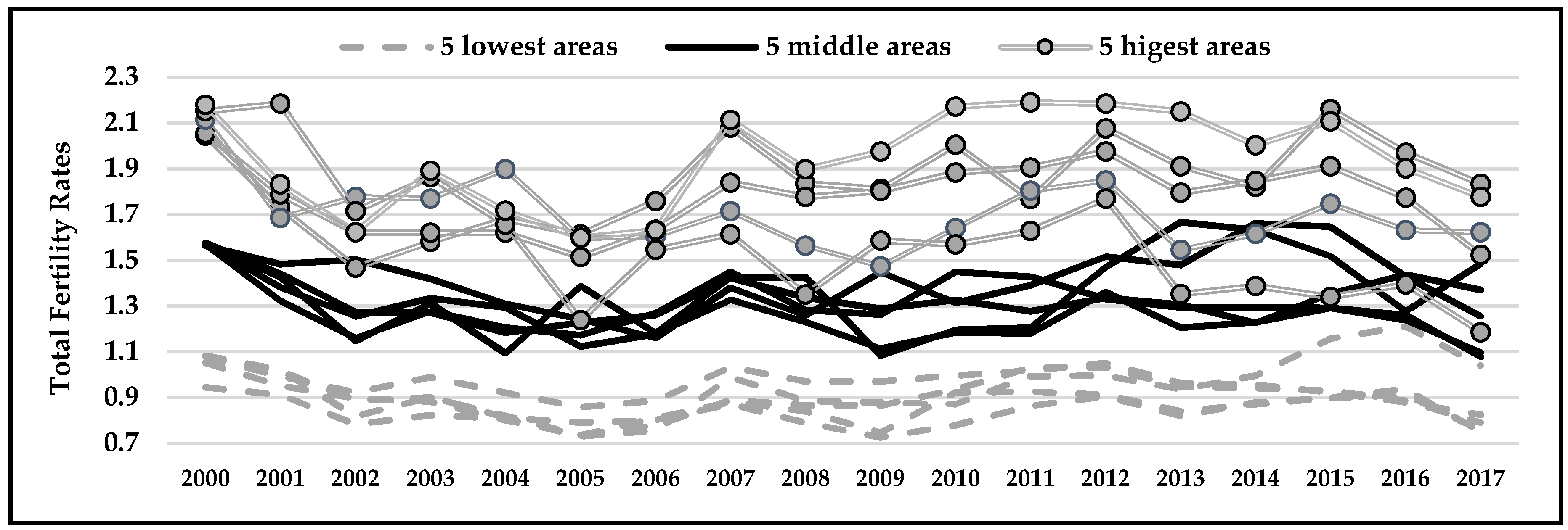
In the last few decades, South Korea has witnessed a remarkable decline in birth rates. Despite the third round of the National Five-Year Plans in pursuit of addressing low-fertility levels since 2006, the total fertility rate (TFR) officially hit 0.98 in 2018 [1]. There has been a large volume of the literature exploring determinants of low fertility in South Korea [2,3,4,5]. However, results of previous studies have varied in terms of the major driving forces and the role of specific factors for fertility declines [6,7,8,9,10]. One reason for the inconsistent results may be derived from variations in the local contexts and characteristics. Although South Korea is known as a relatively homogeneous country, regional fertility levels have not been homogeneous. Figure 1 depicts how local-level TFRs of the five highest, five middle, and the five lowest local areas in 2000 fluctuated until 2017. The figure reveals that changes in local fertility levels were not geographically homogeneous, as local-level TFRs in these areas fluctuated differently in terms of both degree of fluctuation and direction. Instead, it suggests that the fertility-decline process in South Korea is combined with local contexts in which similar sociodemographic factors may result in different fertility outcomes at different places.
In spite of various fertility theories to support fertility variations due to different geographical settings [11], studies examining spatial heterogeneity of fertility in South Korea are scarce. Previous research has shown the regional differences of fertility in South Korea on the basis of the underlying assumption of demographic transition theory [2,12,13], reaching the overriding conclusion that fertility levels were significantly lower in urban areas than rural areas [10,14,15]. While urban–rural analysis shed considerable light on geographical variations in fertility behavior in South Korea, the traditional urban–rural dichotomy is criticized as geographically crude [16]. Lutz further demonstrated that demographic transition theory cannot anticipate the level of fertility in countries at or below replacement fertility, and he remarked that population density in particular has to be included as a variable in studies of regional variation in human fertility [17]. Alternately, social interaction theory argues that fertility and space are closely related because neighboring locations are likely to influence each other through shared cultural and social norms [18,19]. Their argument is that new ideas, innovations, and behaviors are diffused over space through social interactions such as the learning and imitating process. Therefore, such a process takes place in neighboring areas to create spatially similar patterns of fertility, and this process is often independent of urban–rural characteristics [20]. Social interaction theory is also consistent with Tobler’s first law of geography: “Everything is related to everything else, but near things are more related than distant things” [21]. Although several studies have underscored the diffusion effects on fertility decline in South Korea [22,23,24], it is far from clear how the diffusion process spatially occurred. Beyond these causal mechanisms, regional fertility patterns can be explained by migration effects [25]. First, socialization hypothesis says that the fertility behavior of migrants in destination regions reflects fertility preferences in their original regions. Therefore, migrant fertility levels are similar to the fertility levels of the population at the origin regions. Second, adaptation hypothesis states that migrants can be resocialized and adopt the dominant fertility behavior at the destination environment. Third, selection hypothesis explains that people who are inclined to have fewer children possibly migrate to urban areas to enjoy the greater income opportunities offered by cities, and people who are inclined to have more children possibly move to rural areas where costs of raising children are lower. In sum, geographical variations in fertility cannot simply be explained by a single and universal theory because the interconnection between sociodemographic factors and TFRs contains a complex array of local contexts [26].
The development of geographical information systems (GIS) and the increasing availability of georeferencing data have allowed for analyzing spatially heterogeneous patterns of social or demographic phenomena. In dealing with spatial heterogeneity, the Geographically Weighted Regression (GWR) model is particularly relevant to the study of the influence of sociodemographic characteristics on fertility, since the GWR model allows different relationships to exist at different spaces by calibrating multiple regression models using spatial weights [27]. The GWR model can address the specificities of each space and consider that fertility changes in different places may have different responses to changes in sociodemographic variables. Thus, the aim of this study is to conduct spatial analysis and explore spatially heterogeneous relationships between local-level TFRs and sociodemographic factors in South Korea, rather than investigating a global relationship. In order to underpin the application of spatial analysis to regional fertility variations, this paper first examines the spatial autocorrelation of TFRs in South Korea. It then compares the Ordinary Least Squares (OLS) regression model to show global driving factors of TFRs and the GWR model to capture local driving factors. Study findings can thus be expected to attempt to embrace various explanations behind regional fertility differentials and suggest more reasonable and local specific implications for fertility policy-making in South Korea.
2. Materials and Methods
2.1. Data Sources and Study Area
South Korea has 17 province-level administrative divisions, including 1 special city, 1 special autonomous city, 1 special autonomous province, 6 metropolitan cities, and 8 provinces. These divisions are subdivided into 252 local-level divisions, and this study analyzes these 252 local areas. Local-level data were collected from the 2015 Population and Housing Census, which is available at the Korea Statistical Information Service (www.kosis.kr). The 2015 administrative boundary shapefile is linked to the 2015 Population and Housing Census data. The administrative boundary shapefile was obtained from the National Spatial Data Infrastructure Portal (www.nsdi.go.kr).
2.2. Dependent Variable
Total Fertility Rate (TFR) was used as the dependent variable. TFR is defined as the average number of children a woman would bear if she survived through the end of the reproductive age span (15–45), experiencing the age-specific fertility rates of that period at each age. TFR is a period fertility measurement, which is independent of the effect of age structure. Hence, TFR is widely used to compare fertility levels across different places.
2.3. Independent Variables
2.3.1. Number of Childcare Centers
Although the common hypothesis that available, affordable, and acceptable child care should increase fertility has long been part of the research literature [28], empirical studies in the United States and Europe have been inconsistent and often present results that are contrary to hypothetical expectations [29,30,31,32]. Furthermore, Fukai found that an increase in childcare availability in Japan resulted in a small but significant increase in fertility rates only in regions where the propensity for women to work is high, but had no significant effect in other regions [33]. He therefore highlighted that the government should pay attention to regional heterogeneity when formulating childcare policy. In response to low fertility in South Korea, the South Korean government began to provide financial support for promoting childcare availability, rapidly increasing the number of registered childcare centers and kindergartens. However, research results have been inconsistent, showing both the positive and negative effects of the availability of childcare centers on fertility in South Korea [8,9]. Therefore, the number of childcare centers per 1000 children aged 0–5 at the 252 study areas in 2015 was included as an independent variable, which is calculated as (Number of Childcare Centers/Populations Aged 0–5) × 1000.
2.3.2. Female Education
Women’s education is often expected to be associated with delaying or reducing fertility [34,35]. A number of studies has shown that women’s education contributed to delaying marriage and fertility decline in South Korea, although the influence of rising levels of education on fertility decline might be small [6,36]. Despite the general effects of female education on fertility decline, Statistics Korea reported in 2017 that the TFR of female university graduates was higher than female high-school graduates in 2005–2015 [37]. Lee further demonstrated that the period TFR was the lowest for the female population group with the lowest educational category and the highest for the highest educational category, after removing foreign-born women in South Korea [38]. These study results indicate that regional fertility differentials can be caused by the different proportions of female educational levels and, therefore, the proportion of female university graduates aged over 25 at each study areas in 2015 was included as an independent variable.
2.3.3. Population Density
Lutz et al. emphasized that population density is the major determinant of fertility decline [17]. There are different ways in which population density may affect fertility. For Malthus, areas with higher population density cause lower agricultural income, and fertility is delayed (preventive check) compared to areas with lower population density [39]. Sadler et al. explained that, while income is higher in more densely populated areas by agglomeration externalities, fertility decreases, leading to the same final negative relationship between density and fertility [40]. In a modern economy, economists revealed both positive and negative roles of geographical population density for fertility. The positive role of high population density is called “agglomeration economies” [41]. Agglomeration economies often occur in a densely populated region, which results in increasing productivity and wage rate by agglomeration, such as knowledge spill-over across firms and the presence of a more extensive division of labor [42]. As a result, people with more disposable income increase the fertility rate through the positive income effect [43]. On the other hand, agglomeration economies can create negative effects as well by raising the opportunity costs of rearing children through the negative substitution effect [43]. In addition, increased costs of living in densely populated areas may result in “congestion diseconomies”, which reduce disposable income and consequently lower birth rates [44]. These imply that different local contexts may lead to different channels in which population density affects fertility in a negative or positive way. Population density is calculated as Population/Land Area ().
2.3.4. Net Migration Rates
As discussed above in this paper, mobilization of people can cause regional variations in fertility. Therefore, the net migration rate in 2015 was included as an independent variable to assess the migration effect on regional fertility differentials. The net migration rate is measured as ((Number of Immigrants—Number of Emigrants)/Population) × 100. In addition, Sato argues that net migration effects often interact with the effect of population density on fertility variations within a country. He states that a region with stronger agglomeration economies attracts more people to generate congestion diseconomies, which may reduce the region’s fertility rate [45].
2.3.5. International Marriage
The influx of marriage migrants from developing countries to South Korea has increased since 2005, as the Korean government promotes multicultural families as a means to secure the reproductive capacity of the nation [46]. Moreover, another reason for the growth of marriage migrants is the increasing demands for female marriage migrants by men in agricultural areas having difficulties in finding a partner. Lee at al. also demonstrated that growth in international marriages between male South Korean and female Vietnamese individuals has been spurred not only by the ‘marriage squeeze’ in rural areas, but also by the economic motivation of Vietnamese marriage migrants [47]. Therefore, female marriage migrants in South Korea are more likely to settle down in rural areas, and they are expected to have more children. However, empirical studies have shown that Korean–Korean couples experience higher fertility hazards for the first birth and shorter timing for the second birth than foreign couples [48,49]. This study measures the proportion of international marriage as an independent variable in order to explore the different effects of international marriage on fertility at each study area, which is calculated as (Number of Marriages to Foreigners/Number of Marriages) × 100.
2.3.6. Local-Population Growth
Although population growth is regarded as the outcome of fertility changes, this study includes population growth. This is because concerns over the potential risk of so-called “local-population extinction” due to the periodical series of low fertility is rising in local governments [50]. As a result, local governments prioritize policy efforts on achieving targeted population growth and size. Hence, this study attempts to assess how local population growth is associated with local fertility levels for the sake of a sustainable local population size. Population growth is calculated as (Population in 2015 − Population in 2014)/Population in 2014.
2.4. Spatial Auticorrelation
In line with Tobler’s first law of geography, spatial data often display spatial autocorrelation, which means locations close to each other show more similar values than those further apart [51]. Spatial autocorrelation can present a problem for statistical testing because spatially autocorrelated data violate one of the key assumptions of standard statistical analysis, that is, residuals are independent and identically distributed [52]. In order to investigate spatial autocorrelation, Moran’s I index is widely used to test statistics for spatial dependency [53]. The standard Moran’s I statistic is a global measure of spatial autocorrelation, where ‘global’ means the one value for the whole of the study areas [54]. Global Moran’s I can be decomposed into a series of local Moran statistics, which are known as Local Indicators of Spatial Association (LISA) [55]. Global and local Moran indices range between −1 and +1, whereby +1 indicates the perfect clustering of similar values, and –1 presents the perfect clustering of dissimilar values. Local Moran’s I identifies the High–High (HH) clusters and Low–Low (LL) clusters, where geographical clusters have a higher local mean than the global mean or the lower local mean than the global mean. The global mean is the mean value of the z-score for all observations, and the local mean is the z-score of the target location’s neighbors [56]. The formula for Moran’s I is given by the following equation:
2.5. Geographically Weighted Regression Model
The GWR model is local linear regression that allows for examining the spatial variabilities of regression parameters. Global linear regression, for instance, the OLS model, assumes the homogeneous spatial relationship between dependent and independent variables. Therefore, the same stimulus leads to the same response in terms of direction and magnitude in all study areas. The classic global regression model can be expressed as:
where i denotes the i-th location; is the dependent variable; are the coefficients; are the independent variables; represents the error term. However, the relationship between dependent and independent variables can in reality be spatially heterogeneous. In order to capture the spatially varying relationships between variables, the GWR model allows for conducting separate regressions at each location. According to Fotheringham, Brunsdon, and Charlton, the basic equation of the GWR model is as follows [27,57]:
where i denotes the i-th location; is the dependent variable; are the coefficients; are the independent variables; represent the longitude and latitude coordinates of the i-th location; is the error term. As the GWR model is a weighted model in terms of geographical distance, it embeds spatial autocorrelation in the regression. Parameters are estimated by matrix form
where is a vector of local estimation of is the diagonal weighting matrix relative to the position of ; is the vector of the dependent variable. The matrix contains the geographical weights in diagonal and 0 in its off-diagonal elements.
Hence, varies with the change of The assumption is that observations near one another have a greater influence on each other’s parameter estimates than observations farther apart, which coincides with Tobler’s first law. In addition, the choice of weighting is important in the GWR, as it determines how many neighbors are to be included in the matrix. Among various available weighting schemes, this study adopted Gaussian weights and the bi-square weighting function, which are commonly used. The function is as follows:
where is the Euclidean distance between location i, at which parameters are estimated, and specific location p, at which data are observed. b is the bandwidth size that is the maximum distance from regression location i, and b defines how many nearby observations should be included in the matrix. This study determines bandwidth size by adopting the adaptive method [58]. Bandwidth can be optimized by the Akaike Information Criterion (AIC) that can be also used for the comparison of the goodness of fit between global and local regression models. Following the development of georeferencing data and the GIS technique, the GWR model is increasingly used in environmental and social-science studies. Hence, this study explores and compare the OLS and GWR models to investigate the spatial heterogeneity of fertility patterns in South Korea. The descriptive statistics and the OLS model were conducted in R (version 3.5.0). Spatial autocorrelation analysis and the GWR model were handled with ArcGIS (version 10.5).
3. Results
3.1. Descriptive Statistics
Table 1 shows the descriptive statistics of all study variables. The table describes that the local-level TFR, on average, was about 1.33. Three areas with TFRs below 0.9 were all located in the capital. Only four study areas had TFRs higher than the replacement level (TFR 2.1), and they were mostly found in the southwestern part of South Korea, South Jeolla Province. The average number of childcare centers per 1000 children was 17, but disparities between areas in terms of the number of childcare centers were large. For ‘female education’, around 35 percent of the female population aged over 25 had a university education, where a high proportion of female university graduates (>60%) were identified mostly in the capital city. Logged ‘population density’ was significantly high in Seoul and Busan, which are the two most urbanized province-level areas in South Korea. Although the average net migration rate and population growth were about zero, figures largely varied across study areas. The proportion of international marriage was about 6 percent on average, but 20 percent of registered marriages in some areas within rural provinces were international marriage.
3.2. Global OLS Model
Table 2 presents the summary of the OLS results. Overall, the independent variables explain 44% of regional fertility levels, and the AIC was –93.97. In terms of the multicollinearity of the study variables, Variance Inflation Factor (VIF) values show that there are no serious redundancy problems with regard to explanatory variables, as no value was higher than 7.5 [59]. Female education and population density had the expected negative relationships with local-level TFRs in 2015, and both variables were statistically significant. In contrast to general expectations, the number of childcare centers and international marriages showed a negative relationship with local-level TFRs, indicating that the increasing number of childcare centers and more marriages to foreigners decreased local-level TFRs in 2015 after controlling for other study variables. Population growth and net migration rates were positively correlated with local-level TFRs, although net migration was not statistically significant. As discussed above, the global regression model assumes that the relationship between dependent and independent variables is homogeneous at all study areas, which cannot identify the spatial heterogeneity of TFRs. Therefore, the global regression model is unable to assess spatial nonstationarity—the relationships between independent and dependent variables vary over space [27]. The OLS diagnostic results in Table 2 shows that the Koenker (BP) statistic was statistically significant (p < 0.01), which indicates the relationships modeled are not consistent, either due to nonstationarity or heteroskedasticity. In addition, the Jarque–Bera (JB) statistic was also statistically significant (p < 0.01), which shows that OLS model predictions can be biased. Lastly, Moran’s I of the residuals from the OLS model showed that residuals are not statistically random (p < 0.05), which indicates that residuals are spatially correlated. Thus, the OLS model may not be the best approach to investigate the relationship between the selected study variables and local-level TFRs in 2015. Hence, the same independent variables were explored with the GWR model.
3.3. Spatial Autocorrelation and Geographiccal Weighted Regression Model
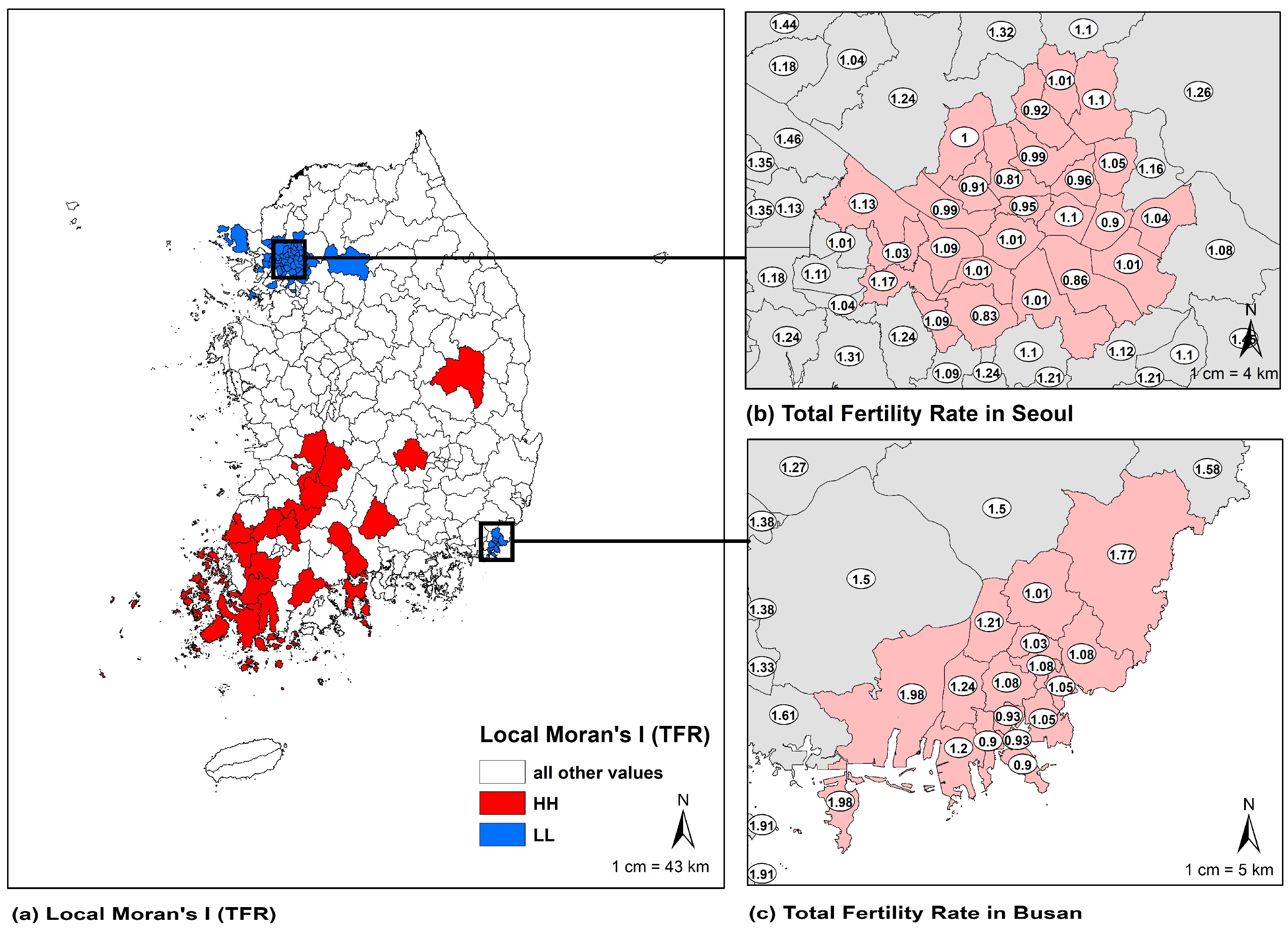
This study calculated the global Moran’s I to assess the spatial autocorrelation of local-level TFRs in South Korea. The global Moran’s I of local-level TFRs was 0.340 (z-score = 28.316, p < 0.001), indicating significant positive spatial autocorrelation of local-level TFRs. In order to further investigate the spatial features of TFR, the local Moran’s I was measured, and Figure 2 shows the local spatial correlation of local-level TFRs. Low–Low (LL) clusters (blue color) were mainly spotted in Seoul and Busan, which are the first and second most populous and urbanized areas in South Korea. High–High (HH) clusters (red color) were found to exhibit geographically scattered distribution. However, HH clusters were mostly displayed in southwestern areas (Jeolla Province), where agricultural areas and aging populations are proportionately high. The spatial autocorrelation of local TFRs in 2015 statistically clarifies the existence of the spatial heterogeneity of fertility levels in South Korea, which thereby requires a locally sensitive regression model.
Table 3 shows the summary of the GWR model. The overall adjusted R-squared value showed that study variables explained 55.4% of local-level TFRs, which is higher than the result in the OLS model (44.0%). In addition, the AIC also improved, from –93.370 in the OLS model to –127.502 in the GWR model. Figure 3 shows the geographical distribution of local R-squared values and the standard deviation of residuals. Local R-squared values were not the same in the study areas, varying between 16.8% and 63.0%. In particular, local R-squared values were higher than the OLS value of 44.5% in northwestern and southeastern areas. The map of the local R-squared values indicates that the relationship between local fertility levels and sociodemographic factors varies across space.
Additionally, the map of standard deviation of residuals shows that the GRW model significantly mitigated spatial autocorrelation problems of the residuals, as standard residuals in most study areas were measured within the range of −1.96 to 1.96 (95% confidence level). Table 3 also presents the percentages of study areas with a statistical significance at 10% for independent variables (t-value > 1.645 or t-value < 1.645), where t-statistics were measured by dividing each local coefficient by the local standard errors of each independent variable [56,60]. As the adaptive method identified 122 neighbors for each local estimation, z-statistics were used to estimate the t-statistics in this study. The table summarizes the descriptive statistics (minimum, maximum, mean, and standard deviation) of coefficients for independent variables. Apart from population growth, all independent variables had both negative and positive coefficients, which was not revealed in the global regression model. Figure 4 displays the distribution of coefficients and the significance level of each independent variable at the study areas. The maps visually demonstrate that the directions, magnitudes, and significance levels of independent variables relative to local-level TFRs vary over space.
The number of childcare centers per 1000 children aged 0–5 revealed the bidirectional effects on local-level TFRs, where around 15 percent of the study areas were positively related to local TFRs. As shown in Figure 4a, positive associations were clustered in areas around the capital city, Seoul, which is consistent with Fukai’s study to show a positive relationship between the availability of childcare centers and TFRs only in regions with high female labor-force participation. Therefore, the increasing number of childcare centers may have increased TFRs around capital cities by improving the life–work balance of the high proportion of working women. Female education (proportion of university graduates) is negatively related to local TFRs in most study areas (96%), which more or less corresponds to the OLS model. This suggests that increases in women’s education are generally associated with lower TFRs. However, Figure 4b shows that positive relations (blue areas) were found in central west areas (North Jeolla Province), where the proportions of the aging population over 60 and agricultural lands are high. In addition, local governments in North Jeolla significantly implement direct cash-transfer programs to avoid a rapidly aging society and promote births. It may suggest that conventional norms about marriage and fertility combined with cash grant programs for births in neighboring areas may partially offset the negative impact of women’s education in North Jeolla. Similarly, population density was negatively related to local-level TFRs in most study areas (98%), with 77% of the study areas being of statistical significance. This finding implies that the negative effects of population density on fertility were dominant in South Korea. However, as shown in Figure 4c, positive effects were recognized around the Jecheon and Chungju areas in North Chungcheong Province. Jecheon and Chungju are located within the landlocked province in the center of South Korea, serving as a major traffic route. Jecheon and Chungju are emerging as the hub for the biomedical industry in South Korea, and housing prices have been in the bottom 20 percentile of the 252 study areas. Thus, one possible explanation for the positive effect of population density is that the inflow of a working-age population seeking job opportunities and low living costs stimulated positive income effects by the ‘agglomeration of economies’ around Jecheon and Chungju in North Chungcheong Province. Despite the few areas with significant t-values, the positive and negative effects of net migration were geographically divided to a large extent. Positive associations (30.56%) were clustered in northeastern and southwestern areas, and negative associations (69.44%) were spotted in northwestern and southeastern areas. This finding is partially consistent with the LISA map in Figure 2a, as negative effects of net migration were found around Seoul and Busan. This suggests that net migration effects on local-level TFRs are slightly consistent with the effects of population density. Increasing population in cities in pursuit of socioeconomic opportunities is incrementally influenced by the negative effects of population density, adopting low fertility behavior in urban cities. In terms of international marriage, the GWR model shows bidirectional effects on local-level TFRs, with about 96 percent negative effects and 4 percent positive effects. This suggests that the socialization effects by marriage migrants were weak in 2015. Instead, marriage migrants were less inclined to have children in South Korea, as marriage migrants were accustomed to a low fertility environment in South Korea, or more marriage migrants were triggered by economic motivation. However, few areas with a positive relationship with local-level TFRs were located around the central–west areas (Daejoen). Daejoen is known as the Silicon Valley of South Korea and also as the home of advanced science- and technology-research institutes. Therefore, in contrast to other areas, foreign migrants in Deajoen are likely to have a higher educational level with better job opportunities, which reasonably leads to different fertility behavior from international couples in other areas in South Korea. Population growth indicates a positive relation with local-level TFRs in all study areas. In addition, almost 95 percent of study areas showed statistical significance, which is consistent with the OLS result. However, the magnitude of the effects varies across space. The effects were relatively low in northern and southwestern areas, where aging populations and agricultural land are proportionately high, and the capital city.
4. Discussion
In order to explore the spatial heterogeneity of fertility in South Korea, this study compares the OLS and GWR models. The result confirms that the relationship between local-level TFRs and the selected sociodemographic factors varies across regions in both magnitude and direction. Although various studies of fertility in South Korea have explored geographical variations in fertility based on rural and urban settings [14,15], this study shows that responses of local-level total fertility rates to sociodemographic factors spatially vary beyond the crude rural and urban dichotomy.
Indeed, the urban–rural dichotomy based on demographic transitional theory is still a powerful explanation for regional fertility differentials in South Korea. The LISA result illustrates that HH patterns of TFRs are spatially clustered around areas of agricultural use, and LL patterns of TFRs are spatially clustered in the two most densely populated and urbanized areas. Moreover, bidirectional effects of net migration rates on TFRs more or less coincides with the result of the LISA map. In other words, the inflow of migrants to LL clustered areas is more likely to be associated with lower fertility due to the strong effects of urbanization and population density, whereas the inflow of migrants to HH clustered areas is positively associated with TFRs, probably due to the light effects of urbanization and population density. Despite the positive effects of population growth on TFRs, the magnitude of their coefficients can vary, possibly owing to the contribution of different age compositions to population growth in urban and rural areas. The magnitude was relatively small in northern and southwestern areas, and around the capital city in 2015. Northern and southwestern areas have high proportions of agricultural lands and elderly populations; therefore, population growth contributed by the elderly population may pose the weak effects on TFRs. Although population growth in the capital city is more likely to be influenced by the younger population, the weak effects of population growth on TFRs could be generated by strong urban effects such as high housing prices and population density. On the other hand, population growth in other areas could be more influenced by a younger population that may create stronger effects on TFRs. In addition, the positive effects of the number of childcare centers per 1000 children on TFRs around the capital city seems to be consistent with Fukai’s result that the availability of childcare centers is only positively related to TFR in urban areas, where female labor-force participation is significantly high [33]. This suggests that the increasing number of childcare centers around the capital city may improve the work–life balance to reduce the opportunity costs of raising children in South Korea.
However, as prior studies have also shown, geographical fertility variations are also caused by the effect of migration regardless of the degree of urbanization [25]; some sociodemographic factors do not comply with the geographical patterns of fertility based on rural–urban gradients in South Korea due to the characteristics of migrants. Although population density poses strong negative effects on TFRs, the GWR model indicates that the positive effects of population density on TFRs can be recognized in certain areas. For example, in this study, Jecheon and Chungju are emerging as the hub for the biomedical industry in South Korea, with a large number of jobs created. Moreover, housing prices around Jecheon and Chungju have been in the bottom 20 percentile of the 252 study areas. As a result, the proportion of an active working-age population, aged 30–59, has increased in the last 10 years in Jecheon and Chungju, and the average marriage age of North Chungcheong Province for both male and female fell to the lowest between the 17 provinces in 2018. The positive effects of population density on TFRs in Jecheon and Chungju correspond to Sato’s arguments that ‘agglomeration of economies’ and ‘congestion diseconomies’ stimulated by net migration from less to more or more to less densely populated areas partially determine the geographical features of fertility [45]. Hence, the influx of an active working-age population to less densely populated areas around Jecheon and Chungju in pursuit of job opportunities and low-living-cost conditions may create positive income effects on fertility through ‘agglomeration of economies’, whereas the effect of ‘congestion diseconomies’ can be relatively offset. In addition, international marriage is often expected to increase fertility levels by the socialization effects of marriage migrants from developing countries [61]. In contrast to general expectations, the negative association between international marriage and local-level TFRs in 2015 reflects that the income motivation of marriage migrants (selection effect) is now strong, or their fertility behaviors have become accustomed to South Korea’s low-fertility environment (adoption effect). Nonetheless, this study shows that international marriage can cause positive effects on TFRs in few areas. For instance, Deajeon, located in the central–western area of South Korea, is known as the Silicon Valley of South Korea, where foreign migrants in Deajeon are often highly educated. High-income and better job opportunities available for them may cause different and procreative fertility behaviors compared to foreign couples in other regions.
In addition to the effects of migration and urbanization, regional fertility differentials could be in part driven by social-interaction effects [18]. For example, female education is known as a major driving force for fertility decline. This study also shows that the high proportion of female university graduates is negatively associated with TFRs in the global model and most study areas in the GWR model. However, female education was positively associated with TFRs around North Jeolla Province in 2015. North Jeolla has high proportions of an elderly population and agricultural lands. Therefore, conventional norms about marriage and fertility behavior may still exist in some areas of North Jeolla. Furthermore, in order to address a rapidly aging society, local governments in North Jeolla actively support the high amount of cash grants to promote births. This may suggest that conventional ideas about fertility behavior, together with the diffusion of strong cash-transfer programs in North Jeolla, may alleviate the negative influence of women’s education on TFRs.
Hence, this study confirms that relationships between local-level TFRs and sociodemographic factors can vary across space, beyond the simple urban–rural dichotomy. Moreover, in accordance with Tobler’s first law of geography, this study visually illustrates how associations between local-level TFRs and sociodemographic factors are spatially clustered and related. However, this study has a few limitations. First, this study only investigates the spatial heterogeneity of fertility patterns for a single year and therefore temporal effects on fertility may be missed. Recently, the geographically and temporal weighted regression (GTWR) model was developed in order to analyze spatial and temporal patterns. Therefore, GTWR should be applied to fertility studies in South Korea. Second, economic or age-specific variables that certainly influence regional fertility variations are not included in this study. More research is required to investigate inclusive driving forces for local-level TFRs. That said, further spatial regression models should be developed that are able to not only investigate spatial variations in fertility, but also deal with the degree of multicollinearity between local-level variables.
5. Conclusions
This study demonstrates that relationships between local-level TFRs and sociodemographic factors are spatially heterogeneous in South Korea. The results can be summarized concisely; the effects of selected socio-demographic factors on TFRs spatially vary across:
Urban and densely populated areas: Low fertility rates were particularly clustered in the two most urbanized and densely populated areas. In addition, net migration rates were negatively associated with TFRs around the two areas. Despite the positive effects of population growth on TFRs, it was exceptionally weak around the capital city due to strong urban effects. Interestingly, the increasing number of childcare centers only raised TFRs around the capital city, possibly by improving the life–work balance of high female labor-force participation. These findings are partially consistent with the urban–rural dichotomy.
Special areas: Although international marriage and population density showed negative effects on local-level TFRs in general, positive effects were identified in Daejeon and around Jecheon and Chungju in North Chungcheong Province, respectively. These areas are characterized by their specialized industries that attract highly educated foreigners to Deajeon and more working-age population to Jecheon and Chungju. These findings imply that it is important to consider who migrates to where [25].
Rural districts: Despite the overall negative effects of higher women’s educational levels on TFRs, women’s education increased TFRs in North Jeolla Province, where proportions of agricultural lands and elderly populations are high. Conventional norms about marriage and fertility, together with the diffusion of strong cash-transfer programs in neighboring areas to promote births, probably offset the effects of women’s education in North Jeolla, which more or less coincides with social-interaction theory.
In conclusion, regional fertility variation in South Korea cannot be explained by a single and universal theory, as different local contexts have to be considered. The policy implication for fertility policy in South Korea is that a one-size-fits-all solution to address persistent low-fertility may be necessary but insufficient in pursuit of a fertility rebound. Instead, local-specific population policies have to be more frequently cultivated. In particular, in the era of geoinformation, spatial analysis including the GWR model should be more applied to population research in South Korea in order to provide evidence-based local policy options.
Author Contributions
Conceptualization, Myunggu Jung and Youngtae Cho; Data curation, Myunggu Jung; Formal analysis, Myunggu Jung; Investigation, Myunggu Jung, Woorim Ko, Yeohee Choi, and Youngtae Cho; Methodology, Myunggu Jung and Youngtae Cho; Software, Myunggu Jung; Supervision, Youngtae Cho; Validation, Youngtae Cho; Visualization, Myunggu Jung; Writing—original draft, Myunggu Jung; Writing—review and editing, Myunggu Jung, Woorim Ko, Yeohee Choi, and Youngtae Cho
Funding
This study was supported by the National Research Foundation of Korea grant funded by the Korean government (No.21B20151213037, 2017R1C1B1004892).
Acknowledgments
The authors would like to thank the anonymous reviewers for their constructive comments that contributed to improving the final version of the paper. They would also like to thank the Editors for their generous support during the review process.
Conflicts of Interest
The authors declare no conflict of interest.
References
- Statistics-Korea. Provisional Result of 2018 Vital Stataststics; Statistics-Korea: Daejeon, Korea, 2018. [Google Scholar]
- Kim, D.-S. Theoretical explanations of rapid fertility decline in Korea. Jpn. J. Popul. 2005, 3, 2–25. [Google Scholar]
- Anderson, T.; Kohler, H.-P. Education fever and the East Asian fertility puzzle: A case study of low fertility in South Korea. Asian Popul. Stud. 2013, 9, 196–215. [Google Scholar] [CrossRef] [PubMed]
- Kim, H.S. Female labour force participation and fertility in South Korea. Asian Popul. Stud. 2014, 10, 252–273. [Google Scholar] [CrossRef]
- Kan, M.-Y.; Hertog, E. Domestic division of labour and fertility preference in China, Japan, South Korea, and Taiwan. Demogr. Res. 2017, 36, 557–588. [Google Scholar] [CrossRef] [Green Version]
- KIHASA. A Study of Fertility Changes in Korea: Based on National Fertility and Family Health Survey (1974–2012); Korea Institute for Health and Social Affairs: Seoul, Korea, 2016. [Google Scholar]
- Kim, J. Female education and its impact on fertility. IZA World Labor 2016, 228, 1–10. [Google Scholar] [CrossRef]
- Seo, M.; Yang, M.; Kang, K. Micro & Macro Approach on Relationship between Child Care Policy and Fertility; Korea Institute for Health and Social Affairs: Seoul, Korea, 2016. [Google Scholar]
- Lee, S.; Choi, H.; Jung, H.E. Evaluation on Effectiveness of Policies in Response to Low Fertility; Korea Institute for Health and Social Affairs: Seoul, Korea, 2010. [Google Scholar]
- Yoo, H.-J.; Hyun, S.-M. The effects of economic resources on marriage-delaying. Korea J. Popul. Stud. 2010, 33, 75–101. [Google Scholar]
- Hirschman, C. Why fertility changes. Annu. Rev. Sociol. 1994, 20, 203–233. [Google Scholar] [CrossRef]
- Lee, S.-S. Low fertility and policy responses in Korea. Jpn. J. Popul. 2009, 7, 57–70. [Google Scholar]
- Jun, B.; Lee, J. The Tradeoff between Fertility and Education: Evidence from the Korean Development Path; FZID Discussion Paper: Stuttgart, Germany, 2014. [Google Scholar]
- Kwon, T.; Kim, T.; Kim, D.-S.; Eun, K.-S. Unerstanding Fertility Transition in Korea; Ilsinsa: Seoul, Korea, 1997. [Google Scholar]
- Lee, S.; Choi, H. Social structural Determinants of Regional Variations in Fertility. Adv. Sci. Technol. Lett. 2016, 131, 60–63. [Google Scholar]
- Kulu, H.; Boyle, P.J. High Fertility in City Suburbs: Compositional or Contextual Effects? Eur. J. Popul. 2009, 25, 157–174. [Google Scholar] [CrossRef]
- Lutz, W.; Testa, M.R.; Penn, D.J. Population density is a key factor in declining human fertility. Popul. Environ. 2006, 28, 69–81. [Google Scholar] [CrossRef]
- Cleland, J.; Wilson, C. Demand theories of the fertility transition: An iconoclastic view. Popul. Stud. 1987, 41, 5–30. [Google Scholar] [CrossRef]
- Bongaarts, J.; Watkins, S.C. Social interactions and contemporary fertility transitions. Popul. Dev. Rev. 1996, 22, 639–683. [Google Scholar] [CrossRef]
- Casterline, J.B.; Population, National Research Council (US) Committee on Population. Diffusion processes and fertility transition: Introduction. In Diffusion Processes and Fertility Transition: Selected Perspectives; National Academies Press (US): Washington, DC, USA, 2001. [Google Scholar]
- Tobler, W.R. A computer movie simulating urban growth in the Detroit region. Econ. Geogr. 1970, 46, 234–240. [Google Scholar] [CrossRef]
- Kwon, T.-H. The Historical Background to Korea’s Demographic Transition; Harvard University Press: Cambridge, MA, USA, 1981; pp. 1–26. [Google Scholar]
- Yoo, S.H. Educational differentials in cohort fertility during the fertility transition in South Korea. Demogr. Res. 2014, 30, 1463–1494. [Google Scholar] [CrossRef] [Green Version]
- Kye, B. Cohort effects or period effects? Fertility decline in South Korea in the twentieth century. Popul. Res. Policy Rev. 2012, 31, 387–415. [Google Scholar] [CrossRef]
- Kulu, H. Migration and fertility: Competing hypotheses re-examined. Eur. J. Popul./Rev. européenne de Démographie 2005, 21, 51–87. [Google Scholar] [CrossRef]
- Courgeau, D. Family formation and urbanization. Popul. Engl. Sel. 1989, 44, 123–146. [Google Scholar]
- Brunsdon, C.; Fotheringham, A.S.; Charlton, M.E. Geographically weighted regression: A method for exploring spatial nonstationarity. Geogr. Anal. 1996, 28, 281–298. [Google Scholar] [CrossRef]
- Myrdal, A. Nation and Family; the Swedish Experiment in Democratic Family and Population Policy; MIT Press: Cambridge, MA, USA, 1968. [Google Scholar]
- Rindfuss, R.R.; Guzzo, K.B.; Morgan, S.P. The changing institutional context of low fertility. Popul. Res. Policy Rev. 2003, 22, 411–438. [Google Scholar] [CrossRef]
- Blau, D.M.; Robins, P.K. Fertility, Employment, and Child-Care Costs—A Dynamic Analysis. Popul. Index 1986, 52, 393. [Google Scholar]
- Mason, K.O.; Kuhlthau, K. The Perceived Impact of Child-Care Costs on Womens Labor Supply and Fertility. Demography 1992, 29, 523–543. [Google Scholar] [CrossRef] [PubMed]
- Rindfuss, R.R.; Guilkey, D.K.; Morgan, S.P.; Kravdal, O. Child-Care Availability and Fertility in Norway. Popul. Dev. Rev. 2010, 36, 725–748. [Google Scholar] [CrossRef] [PubMed]
- Fukai, T. Childcare availability and fertility: Evidence from municipalities in Japan. J. Jpn. Int. Econ. 2017, 43, 1–18. [Google Scholar] [CrossRef]
- Bongaarts, J. Completing the fertility transition in the developing world: The role of educational differences and fertility preferences. Popul. Stud. 2003, 57, 321–335. [Google Scholar] [CrossRef] [PubMed]
- Caldwell, J.C. Mass Education as a Determinant of the Timing of Fertility Decline. Popul. Dev. Rev. 1980, 6, 225–255. [Google Scholar] [CrossRef]
- Choe, M.K.; Retherford, R.D. The contribution of education to South Korea’s fertility decline to ‘lowest-low’ level. Asian Popul. Stud. 2009, 5, 267–288. [Google Scholar] [CrossRef]
- Statistics-Korea. Analysis of Birth, Death, Marriage and Divorce by Educational Level: 2000–2015; Statistics Korea: Daejeon, Korea, 2017. [Google Scholar]
- Lee, E. Educational differences in period fertility: The case of South Korea, 1996–2010. Demogr. Res. 2018, 38, 309–320. [Google Scholar] [CrossRef]
- Malthus, T.R. An Essay on the Principle of Population: Or, a View of its Past and Present Effects on Human Happiness, with an Inquiry into Our Prospects Respecting the Future Removal or Mitigation of the Evils Which It Occasions; Reeves and Turner: London, UK, 1878. [Google Scholar]
- Sadler, M.T. The Law of Population: A Treatise, in Six Books; in Disproof of the Superfecundity of Human Beings, and Developing of the Real Principle of Their Increase; Murray, J., Ed.; Nabu Press: Charleston, SC, USA, 2011. [Google Scholar]
- Morita, T.; Yamamoto, K. Economic Geography, Endogenous Fertility, and Agglomeration; Research Institute of Economy, Trade and Industry (RIETI): Tokyo, Japan, 2014. [Google Scholar]
- Fujita, M.; Thisse, J.-F. Economics of Agglomeration: Cities, Industrial Location, and Globalization; Cambridge University Press: Cambridge, UK, 2013. [Google Scholar]
- Becker, G.S. An economic analysis of fertility. In Demographic and Economic Change in Developed Countries; Columbia University Press: New York, NY, USA, 1960; pp. 209–240. [Google Scholar]
- Richardson, H.W. Economies and diseconomies of agglomeration. In Urban Agglomeration and Economic Growth; Springer Science & Business Media: Berlin, Germany, 1995; pp. 123–155. [Google Scholar]
- Sato, Y. Economic geography, fertility and migration. J. Urban Econ. 2007, 61, 372–387. [Google Scholar] [CrossRef]
- Kim, G.; Kilkey, M. Marriage Migration Policy in South Korea: Social Investment beyond the Nation State. Int. Migr. 2018, 56, 23–38. [Google Scholar] [CrossRef]
- Lee, H.; Williams, L.; Arguillas, F. Adapting to Marriage Markets: International Marriage Migration from Vietnam to South Korea. J. Comp. Fam. Stud. 2016, 47, 267–288. [Google Scholar] [CrossRef]
- Kim, H.-S.; Kim, K.; Jun, K.-H. Mate Selection Pattern and Fertility Differentials among Married Immigrants in Korea. In Cross-Border Marriage: Global Trends and Diversity; Korea Institute for Health and Social Affairs: Seoul, Korea, 2012; pp. 235–278. [Google Scholar]
- Kim, H.S. Fertility differentials between Korean and international marriage couples in South Korea. Asian Popul. Stud. 2018, 14, 43–60. [Google Scholar] [CrossRef]
- Lee, S.-l.; Yi, J. Fertility and the Proportion of Newlyweds in Different Municipalities. KIHASA Res. Brief 2018, 32, 1–6. [Google Scholar]
- Dormann, C.F.; McPherson, J.M.; Araújo, M.B.; Bivand, R.; Bolliger, J.; Carl, G.; Davies, R.G.; Hirzel, A.; Jetz, W.; Daniel Kissling, W.; et al. Methods to account for spatial autocorrelation in the analysis of species distributional data: A review. Ecography 2007, 30, 609–628. [Google Scholar] [CrossRef]
- Legendre, P. Spatial autocorrelation: Trouble or new paradigm? Ecology 1993, 74, 1659–1673. [Google Scholar] [CrossRef]
- Tiefelsdorf, M. The saddlepoint approximation of Moran’s I’s and local Moran’s I’s reference distributions and their numerical evaluation. Geogr. Anal. 2002, 34, 187–206. [Google Scholar] [CrossRef]
- Harris, R. Quantitative Geography; Sage Publication Ltd.: London, UK, 2016. [Google Scholar]
- Anselin, L. Local indicators of spatial association—LISA. Geogr. Anal. 1995, 27, 93–115. [Google Scholar] [CrossRef]
- Wang, S.; Shi, C.; Fang, C.; Feng, K. Examining the spatial variations of determinants of energy-related CO2 emissions in China at the city level using Geographically Weighted Regression Model. Appl. Energy 2019, 235, 95–105. [Google Scholar] [CrossRef]
- Fotheringham, A.S.; Oshan, T.M. Geographically weighted regression and multicollinearity: Dispelling the myth. J. Geogr. Syst. 2016, 18, 303–329. [Google Scholar] [CrossRef]
- Fotheringham, A.S. Trends in quantitative methods I: Stressing the local. Prog. Hum. Geogr. 1997, 21, 88–96. [Google Scholar] [CrossRef]
- Neter, J.; Kutner, M.H.; Nachtsheim, C.J.; Wasserman, W. Applied Linear Statistical Models; McGraw-Hill & Irwin: Chicago, IL, USA, 1996. [Google Scholar]
- Chasco Yrigoyen, C.; García, I.; Vicéns, J. Modeling Spatial Variations in Household Disposable Income with Geographically Weighted Regression; University Library of Munich: Munich, Germany, 2007. [Google Scholar]
- Toulemon, L. Fertility among immigrant women: New data a new approach. Popul. Soc. 2004, 400, 1–4. [Google Scholar]
Figure 1.
Fluctuation of local-level total fertility rates (TFRs).

Figure 2.
(a) Local Moran’s I of local TFRs; (b) TFRs in Seoul; (c) TFRs in Busan.

Figure 3.
(a) R-squared values; (b) standard deviation of residuals.

Figure 4.
Spatial distribution of GWR local coefficients: (a) Childcare Centers; (b) Female Education; (c) Population Density; (d) Net Migration; (e) International Marriage; (f) Population Growth.
Figure 4.
Spatial distribution of GWR local coefficients: (a) Childcare Centers; (b) Female Education; (c) Population Density; (d) Net Migration; (e) International Marriage; (f) Population Growth.


Table 1.
Descriptive statistics (in 2015).
| Category | Variable | Mean | Std. Dev. | Min. | Max. |
|---|---|---|---|---|---|
| Dependent variable | Total Fertility Rate | 1.33 | 0.26 | 0.81 | 2.46 |
| Independent variable | Childcare Centers (per 1000) | 17.48 | 4.27 | 7.38 | 31.79 |
| Female Education (%) | 35.24 | 11.42 | 18.36 | 79.15 | |
| (log) Population Density | 2.84 | 0.94 | 1.25 | 4.42 | |
| Net Migration Rate (%) | 0.112 | 2.026 | –4.4 | 16.3 | |
| International Marriage (%) | 6.25 | 3.10 | 2.45 | 20.00 | |
| Population Growth (%) | 0.39 | 1.96 | –3.05 | 15.51 |
Table 2.
Summary of Ordinary Least Squares (OLS) statistics.
| Variable | Coefficient | Std. Error | t-Value | p-Value | VIF | |
|---|---|---|---|---|---|---|
| Constant | 2.04 *** | 0.098 | 20.763 | 0.000 | — | |
| Childcare Center (per 1000 children) | –0.009 *** | 0.003 | –2.820 | 0.000 | 1.129 | |
| Female Education (%) | –0.005 *** | 0.001 | –3.338 | 0.000 | 1.929 | |
| (log) Population Density () | –0.122 *** | 0.020 | –6.093 | 0.000 | 2.307 | |
| Net migration Rate (%) | 0.001 | 0.006 | 0.107 | 0.914 | 1.022 | |
| International Marriage (%) | –0.009 * | 0.005 | –1.681 | 0.094 | 1.766 | |
| Population Growth (%) | 0.042 *** | 0.007 | 6.299 | 0.000 | 1.067 | |
| OLS Diagnostics | AIC | –93.37 | Koenker(BP) | 34.584 *** | Moran’s I | 0.035 *** |
| Adj | 0.440 | Jarque–Bera | 122.996 *** | |||
Note: *** significant at 1% level; ** significant at 5% level; * significant at 10% level.
Table 3.
Summary of Geographically Weighted Regression (GWR) statistics.
| Variable | GWR Coefficients | % of (+) or (−) Coefficients | % of t-Values | ||||
|---|---|---|---|---|---|---|---|
| Min | Max | Mean | Std. | (+) | (−) | p < 0.1 | |
| Childcare Centers (per 1000 children) | −0.027 | 0.005 | −0.007 | 0.008 | 15.08% | 84.92% | 30.95% |
| Female Education (%) | −0.012 | 0.003 | −0.006 | 0.003 | 3.97% | 96.03% | 81.75% |
| (log)Population Density () | −0.159 | 0.046 | −0.104 | 0.041 | 1.98% | 98.02% | 77.38% |
| Net Migration Rate (%) | −0.014 | 0.025 | −0.002 | 0.005 | 30.56% | 69.44% | 0.79% |
| International Marriage (%) | −0.059 | 0.003 | −0.002 | 0.013 | 3.57% | 96.43% | 55.95% |
| Population Growth (%) | 0.015 | 0.076 | 0.044 | 0.013 | 100% | 0% | 94.84% |
| GWR Diagnostics | Adj | 0.548 | AIC | −127.502 | |||
© 2019 by the authors. Licensee MDPI, Basel, Switzerland. This article is an open access article distributed under the terms and conditions of the Creative Commons Attribution (CC BY) license (http://creativecommons.org/licenses/by/4.0/).
Share and Cite
MDPI and ACS Style
Jung, M.; Ko, W.; Choi, Y.; Cho, Y. Spatial Variations in Fertility of South Korea: A Geographically Weighted Regression Approach. ISPRS Int. J. Geo-Inf. 2019, 8, 262. https://0-doi-org.brum.beds.ac.uk/10.3390/ijgi8060262
AMA Style
Jung M, Ko W, Choi Y, Cho Y. Spatial Variations in Fertility of South Korea: A Geographically Weighted Regression Approach. ISPRS International Journal of Geo-Information. 2019; 8(6):262. https://0-doi-org.brum.beds.ac.uk/10.3390/ijgi8060262
Chicago/Turabian StyleJung, Myunggu, Woorim Ko, Yeohee Choi, and Youngtae Cho. 2019. "Spatial Variations in Fertility of South Korea: A Geographically Weighted Regression Approach" ISPRS International Journal of Geo-Information 8, no. 6: 262. https://0-doi-org.brum.beds.ac.uk/10.3390/ijgi8060262
Note that from the first issue of 2016, this journal uses article numbers instead of page numbers. See further details here.