Evaluation of Topological Consistency in CityGML †


Institute of Photogrammetry and Remote Sensing, Karlsruhe Institute of Technology (KIT), Englerstr. 7, 76131 Karlsruhe, Germany
*
Author to whom correspondence should be addressed.
†
This paper is an extended version of our paper published in the proceedings of the ISPRS Technical Commission IV Symposium 2018.
ISPRS Int. J. Geo-Inf. 2019, 8(6), 278; https://0-doi-org.brum.beds.ac.uk/10.3390/ijgi8060278
Submission received: 4 April 2019
/
Revised: 3 June 2019
/
Accepted: 8 June 2019
/
Published: 14 June 2019
(This article belongs to the Special Issue Multidimensional and Multiscale GIS)
Abstract
:Boundary representation models are data models that represent the topology of a building or city model. This leads to an issue in combination with geometry, as the geometric model necessarily has an underlying topology. In order to allow topological queries to rely on the incidence graph only, a new notion of topological consistency is introduced that captures possible topological differences between the incidence graph and the topology coming from geometry. Intersection matrices then describe possible types of topological consistency and inconsistency. As an application, it is examined which matrices can occur as intersection matrices, and how matrices from topologically consistent data look. The analysis of CityGML data sets stored in a spatial database system then shows that many real-world data sets contain many topologically inconsistent pairs of polygons. It was observed that even if data satisfy the val3dity test, they can still be topologically inconsistent. On the other hand, it is shown that the ISO 19107 standard is equivalent to our notion of topological consistency. In the case when the intersection is a point, topological inconsistency occurs because a vertex lies on a line segment. However, the most frequent topological inconsistencies seem to arise when the intersection of two polygons is a line segment. Consequently, topological queries in present CityGML data cannot rely on the incidence graph only, but must always make costly geometric computations if correct results are to be expected.
1. Introduction
Spatial data models that are designed for the purpose of analysis beyond mere visualisation need the following properties:
- correctness,
- consistency.
Correctness refers here to correctness of geometry and of topology. If data are stored redundantly, then consistency issues arise. However, storing data without redundancy does not guarantee consistency. For example, CityGML has a geometry model and a separate topology model. As geometry itself has an underlying topology, it follows that, by design, CityGML does not guarantee the absence of contradictions between the topology coming from geometry and its topological model. It is the scope of this article to exhibit the carelessness with respect to this kind of topological consistency when CityGML is used for modelling spatial data.
Topological queries like “find all objects at the boundary of object A” or “how close are objects A and B topologically”, where topological nearness of A and B means that there is a short sequence , , ..., such that is in the boundary of or is in the boundary of , can be expected to be most efficiently answered by using the incidence graph of the topological model for given spatial data. The incidence graph is a structure that models the relation “is bounded by”, and answering those queries ideally need not resort to the application of geometric operations like intersection because the incidence graph correctly models the topology. Geometric operations become costly especially when many objects are geometrically close, but topologically not. On the other hand, if objects are topologically near but not geometrically, then they are not considered for the topological query if geometry is used as a basis. Index structures based on Euclidean geometry (like e.g., R-tree) become sub-optimal because they need to take into account objects that are further away than necessary. Thus, a desideratum is a topological index that relies on the topological model only, ignoring the underlying geometry. This is the topic of ongoing work. A necessary condition for the correctness of such an approach is that the topology underlying the geometrical model coincides with that of the topological model. In other words, it is assumed that the model is topologically consistent, a notion that will be made more precise in this article.
CityGML has become a widespread format for urban building data in various levels of detail (LoDs). Biljecki et al. [2] give an overview of different applications of 3D city models. If the data stored in CityGML is to be used for efficient analysis beyond visualisation, they are necessary to be topologically consistent. Otherwise, topological queries yield incorrect results. However, in this present study it turns out that real-world CityGML datasets mostly have different kinds of topological inconsistencies.
The incidence graph is a finite representation of the topology of a spatial model. It has a simple relational database representation through one table for the objects, and another for the topology-defining relation [3]. It is also shown that its storage complexity is quadratic in the number of objects, and this is in general the most efficient to be expected [4]. Furthermore, this data model is universal in that it captures any possible finite topological representation of data [3]. The literature contains various differing notions of topological consistency, cf. e.g., [5,6,7,8]. Bradley [9] gives an overview of topological data models and introduces topological consistency in the context of smart cities. Jahn et al. [10] give a first definition of topological consistency which relates geometry and the incidence graph in the context of distributed big geographical data, and define a measure for topological inconsistency based on Betti numbers of finite partially ordered sets. Alam et al. [11] have a list of consistency rules for topology and semantics in which they do not allow more than two polygons to have a common edge. Gröger and Plümer [12] require a consistent model to represent a finite tesselation of . This excludes polygons not bordering a solid, like e.g., a building with free walls. Ledoux and Meijers [13] define a notion of topological consistency which is a special case of the one considered here. They, for example, do not allow polygons with holes or punctures, and they develop an algorithm for extruding planar polygons for serving as building models. Biljecki et al. [14] reduce redundancies in synthetic CityGML data and thus improve the topological consistency.
Applications of such topological consistency are shown, e.g., in Steuer et al. [15], where the volume of buildings in CityGML is approximated by overcoming topological errors. This approach is useful for indoor routing and healing of building models. In general, we emphasise that any topological query in one way or the other makes use of the underlying topology and thus naturally can be applied to the incidence graph in the case that the data are topologically consistent in our sense.
The contribution of this article can be summarised as follows:
- A new definition of topological consistency that ensures the equality of the incidence graph and the topology coming from geometry,
- In contrast to the definitions in the literature, all possible incidence graphs are accepted as topologically consistent, if the above requirement is fulfilled,
- A definition of intersection matrices for capturing the possible types of topological consistency and inconsistency,
- A deduction of which intersection matrices can possibly occur, and which intersection matrices come from topologically consistent data,
- An analysis of intersection matrices for polygon pairs in various CityGML data sets,
- The fact that complying with the ISO 191907 standard guarantees topological consistency and vice versa.
The latter result means that consistency evaluation methods based on the ISO 19107 standard can detect all kinds of topological inconsistencies. However, correctly modeled CityGML data are not required to be topologically consistent. Hence, costly geometric computations are needed for evaluating topological queries in CityGML.
The literature contains methods for checking topological consistency based on checking for errors contained in a proper subset of all possible errors. One prominent example for this turns out to be val3dity [16]. Hence, one can conclude that passing the val3dity test does not necessarily mean the data to comply with the ISO 19107 standard.
In Section 2, we explain first how topology and geometry are modelled in CityGML, followed by a detailed introduction to our notion of topological consistency. The intersection matrix is then introduced as a first means for recognising topological consistency and distinguishing between different types of topological inconsistencies when the configuration consists of two polygons. Section 3 contains our results for a collection of CityGML data sets, followed by a discussion in Section 4 and a conclusion and outlook in Section 5.
2. Methodology
After an explanation of how topology is modelled in CityGML, we will give a definition of topological consistency which is given if and only if the topology of the incidence graph coming from a boundary representation of geometry coincides with the topology underlying the geometry. An intersection matrix then shows which primitive types (point, line, polygon, etc.) have a non-empty intersection with other primitive types. In the end, we explain how this concept was implemented in order to evaluate CityGML data.
2.1. Topology in CityGML
The geometrical and topological models of CityGML are closely related [17,18]. The spatial properties of CityGML objects are represented by objects of the geometry model of the Geography Markup Language (GML3) [19]. This model is based on the ISO Standard 19107 “Spatial Schema”, which represents three-dimensional geometries according to the well-known Boundary Representation [20]. The GML3 geometry model consists of primitives that can be combined to form complexes, composite geometries, or aggregates. For every dimension, there is a geometrical primitive, such as Point, Curve, Surface and Solid. Points are represented as coordinate triples. The representation of surfaces and curves is restricted to planar polygons. Planar polygons are given by lists of coordinate triples which form the outer and inner boundaries. All coordinates of the outer boundary and of the optional inner boundaries (forming holes in the polygon) must be located in the same plane. Similarly, only straight lines, complying with the GML3 class LineString, are allowed in CityGML.
On the other hand, CityGML provides the explicit modelling of topology, for example the sharing of geometry objects between features or other geometries. One part of space should be represented only once by a geometry object and be referenced by all features or more complex geometries which are defined or bounded by this geometry object. Thus, redundancy should be avoided and explicit topological relationships between the parts should be preserved. Instead of implementing topology with own XML-tags, CityGML uses the XML concept of XLinks, which is provided by GML3. However, there is no need to model the topology in this way to get a valid CityGML file.
We see from the explanations above that there are two competing topological models in CityGML: the one derived from the boundary representation of geometry, and the one provided by the XLink concept. It is now obvious that it is easy to model topological contradictions, i.e., CityGML is by design not consistent. In the following subsections, we will see that it is possible to violate consistency even by using the boundary representation model only.
2.2. Topological Consistency
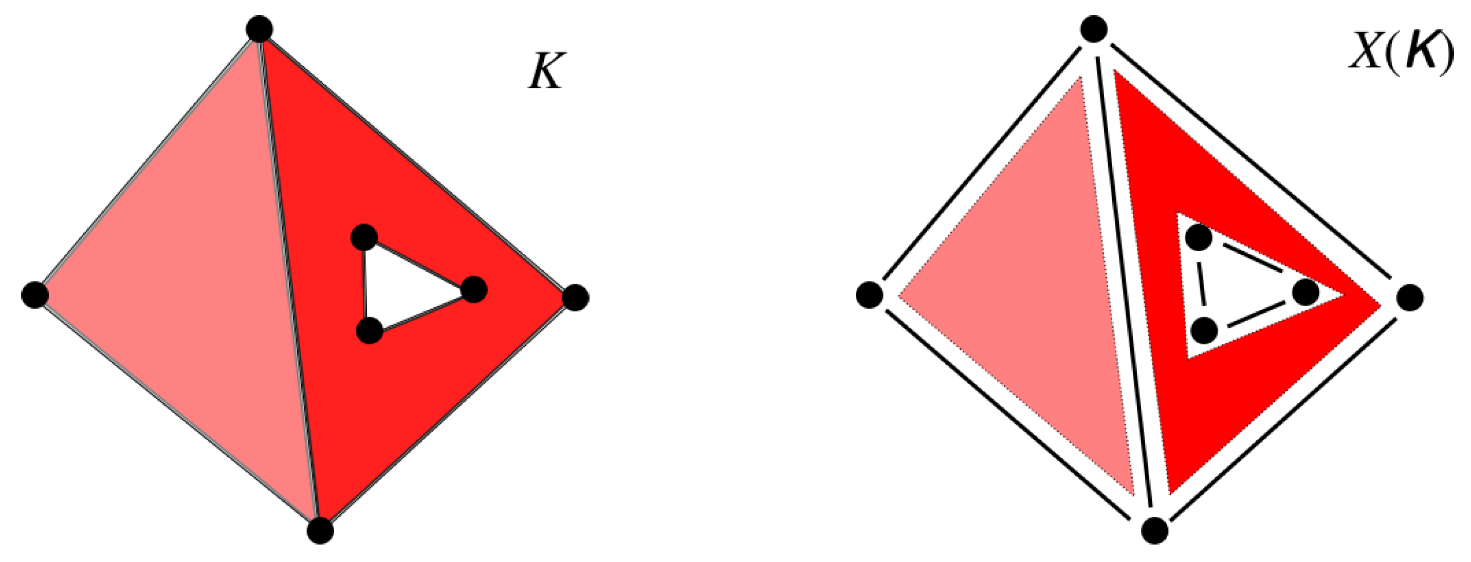
Spatial models of geometry can be finite. For this, the geometry K is partitioned into pieces (often these are cells), and then each piece is considered as an element of a finite set X. In order to model the boundary relationship between the pieces, a topology is defined on the finite set X which represents that boundary relationship. It turns out that X becomes a partially ordered set (aka poset). This allows for using the finite poset X alone for topological queries on K without resorting to the geometry in K. Figure 1 illustrates this process, where a configuration of two polygons forms a partition of geometry K (left) into points, lines and surfaces as the pieces (called faces). The finite poset is illustrated in Figure 1 (right), where the individual faces are now considered as elements without any further structure by themselves. Structure is given by the partial ordering called bounded by, where a face f is bounded by another face , if the piece corresponding to is part of the boundary of the piece F corresponding to f. Consistency issues arise, when a geometry K is given by a configuration of several geometric objects, as then it may happen that K is not a partitioning because pieces overlap. The remainder of this section is devoted to developing the theory which makes this aspect of the topology of spatial entities precise, leading to a general definition of topological consistency.
Consider a topological model of spatial objects modelled as a polytope complex, i.e., a cw complex [21] whose (open) cells are the interiors of polytopes of various dimensions. Assume that all vertices are given coordinates. The incidence graph represents the topology of the model correctly, if and only if the intersection of two distinct open cells is empty. The topology of the incidence graph is that of a finite partially ordered set X, where the partial order is given by the “bounded-by”-relation:
This is a so-called -topology. It is well-known that the -topologies on a finite set are in one-to-one correspondence with the partial orders on that set [22].
We are aware of the fact that our main reference [22] for finite topological spaces is in German. Readers who are not willing to struggle with that language can find the results of that article needed for the present article in the beginning of [23] which deals with topics far more deeper than what is relevant for the task of the present article. We want to remark, however, that most articles on the theory of finite topological spaces usually cite results in [22] without translating the proofs into English, when it comes to presenting the basic results of that theory.
We also want to remark that in this subsection; we use some standard notions from topology which we do not always explain. The reader who would like to learn about the relevant definitions from topology is referred to textbooks on topology, e.g., [24].
The relationship between cw complexes and finite -topolgies is as follows. If is a cw-complex, then there is a surjective map
where X is the finite set whose elements are the cells of . The topology on X is the final topology of (cf. [24]), and it turns out that this is given by the -topology as described above [25]. We are going to develop this idea more precisely in what follows.
A cw complex has for each n-cell c of a so-called characteristic map
which is a continuous map from the n-ball to , and which takes the interior of homeomorphcially to c, and the boundary of to the union of k-cells of with . We will assume that the restriction of to the boundary of is a homeomorphism onto its image. A cw complex satisfying this condition is called regular.
Lemma 1.
The final topology on X for π coincides with the -topology given by ≤.
Proof.
First, we will prove that is continuous, if X is given the -topology induced by ≤. For this, let
This is the unique minimal open neighbourhood of x w.r.t. the -topology [22]. Now, if is a k-cell, then
is the union of with the union of all m-cells with and containing in their boundaries. This is an open set for the topology on [21]. As the form a basis for the -topology on X [22], it follows that is continuous, if X is given the -topology.
Now, we will show that is open, i.e., maps open sets to open sets, if X is given the -topology induced by ≤. Let be an open set. For , let be the unique cell containing x. Then, for
it holds true that
Now, V is the union of open neighbourhoods of points that are minimal with respect to the condition that they are unions of cells. It follows that
is the minimal open neighbourhood of . Hence, is the union of , i.e., open.
As is continuous and open, if X is given the -topology, it follows that this is the final topology for . Namely, if is a topology on X such that is continuous, let be open w.r.t. . As is continuous, it follows that is open in . As is open for the topology on X given by ≤, it follows that is open for this -topology. Hence, the topology given by ≤ is finer than . □
The elements of this -topological space X we also call cells. The space X is called the cell poset of , and the map is called the canonical cell map.
We are interested in the closure of cells:
Lemma 2.
It holds true that
for .
Proof.
This is proved in [22]. □
An important example is that of polyhedra. Let P be a polyhedron in . It has an associated regular cw-complex whose cells are the open faces of P. We denote the cell poset of as and call it the face poset of P. If an n-face f of P is allowed to have k holes, then it is no longer a cell, but there is also a cell-like complex associated with P, called face complex, which is obtained for this face by a continuous map of the unit ball with k holes to P such that the interior maps homeomorphically to f, and the boundary maps homeomorphically into the union of the ℓ-faces of P with . Thus, this is a generalisation of regular cell complex to the case of cells having holes.
Again, there is the face poset with the canonical face map
which is continuous and open (the proof of Lemma 1 carries over to this more general case).
Now, we assume to be a finite set of polyhedra in , possibly with holes which are open polyhedra. We call a configuration. We define
and endow it with the -topology given by the following partial ordering ≤:
where is the partial ordering defining the -topology on .
In contrast to the case of a cw complex or a poyhedron with holes, there is in general not a natural continuous projection .
Definition 1.
A configuration is topologically consistent, if
for every .
This definition is equivalent to the existence of a canonical face map:
Lemma 3.
A configuration is topologically consistent, if and only if the map
is well-defined, where
and is the face containing x. In this case, K can be given the structure of a face complex whose ‘cells’ are homeomorphic to balls with finitely many holes.
Proof.
is topologically consistent, if and only if K is partitioned into faces of polygons from with holes. This is equivalent to being well-defined. In this case, the face complex structure is given by imitating a regular cw complex structure, only that the characteristic maps are from balls with holes instead of just balls. □
This notion leads to a method of deciding whether a configuration of cells is a true cw or face complex by inspecting the finite topological space .
For example, let consist of two distinct polygons P and whose cells are the faces, edges and vertices. Assume that a vertex v of P lies in the interior of an edge e of . Then, has overlapping cells, and thus K is not a cw complex. On the other hand, we have in that
This means that is not topologically consistent.
The definition of topological consistency here extends the definition of [9] and differs from that of [10] or [26]. Observe that our definition of topological consistency also includes the situation where the ‘cells’ of a complex are allowed to have polytope-shaped holes. In that case, it is the topology of the incidence graph which is correctly represented by the model, if and only if it is topologically consistent. Notice that the model can consist of a single, a few, or many objects which may or may not form one or several buildings.
The philosophy behind our definition of topological consistency is that the incidence graph coming from the boundary representation models the “desired” topology, whereas the actual geometric embeddings of the primitives (by giving their corners coordinates) produces a topology which may be different from the incidence graph topology. This idea is captured in the definition of geometric realization ([27], Section 4.49):
and this is what we also mean when we say that the topology coming from geometry coincides with the topology of the incidence graph.“geometric complex whose geometric primitives are in a 1-to-1 correspondence to the topological primitives of a topological complex, such that the boundary relations in the two complexes agree”
An analysis of CityGML data showed that it is possible to have topologically inconsistent models in CityGML with or without using XLink (cf. Section 2.1).
2.3. Comparison with Other Notions of Topological Consistency
The introduction refers to several different notions of topological consistency in the literature, and some possible but consistent situations which they do not capture. It follows that the notion of topological consistency in the literature implies topological consistency in our sense, but not every configuration which is topologically consistent in our sense is topologically consistent in the literature.
Another issue is the kind of topological consistency inherent in the ISO 19107 standard. A validation tool for ISO/OGC standards is given by the tool val3dity. An inspection of the list of possible errors which val3dity can find reveals that not all configurations passing the val3dity test are topologically consistent in our sense. In the following subparagraph, we give some examples.
Comparison with the ISO 19107 Standard and Val3dity
In Section 4.45 of [27], the notion of geometric complex is defined as a
“set of disjoint geometric primitives where the boundary of each geometric primitive can be represented as the union of other geometric primitives of smaller dimension within the same set”.(emphasis added by the authors)
An immediate consequence of the disjointness requirement is
Theorem 1.
Any configuration complies with the ISO 19107 standard if and only if it is topologically consistent.
A common publically available tool for comparing with the ISO/OGC standards is val3dity [16]. Consulting the documentation of val3dity reveals a long list of possible errors. We find that there are some errors not contained in that list, as they are not considered to be errors by val3dity. For example, when a pair of distinct shells is taken, the following constraints are not captured:
- Vertex with Face. A Vertex of a A may not have a non-empty intersection with a face of B.
- Edge with Edge. A non-empty intersection of an edge of A with an edge of B must be an edge both of A and B.
- Edge with Face. An edge of A may not have a non-empty intersection with a face of B.
- Face with Face. A non-empty intersection of a face of A with a face of B must be a face of both A and B.
These constraints follow from the disjointness requirement in the definition of geometric complex in the ISO 19107 standard. Thus, we have
Corollary 1.
If a configuration passes the val3dity test, it is not necessarily topologically consistent.
Proof.
This is an immediate consequence of Theorem 1 and our observation on the non-captured errors. □
One can easily see that these consistency rules must be satisfied, if one wants to use the incidence graph e.g., for querying connectedness: If in A and B there are no common vertices, edges or faces, then the two shells are not connected, unless they violate the above rules. These consistency rules are satisfied by our notion of topological consistency.
2.4. Intersection Matrix
Based on the definition of topological consistency in Section 2.2, it becomes clear that it is necessary to intersect each polygon P with each other polygon to check the topological consistency. For this purpose, we define an intersection matrix as follows in two steps: Let be two configurations in , and let be their corresponding face posets as in in Section 2.2. Then, we define the matrix
Now, there is a map
where is the dimension of face x. Now, there is an induced matrix
We call this matrix the intersection matrix for and . If , then we will write
instead of in order to emphasise it as a symmetric square matrix.
In this study, we are mainly interested in the (symmetric) intersection matrix , where , respectively , is the configuration of the faces, edges and vertices of polygons P, respectively . Notice that we can write
where stands for vertex, stands for edge, and stands for face. The above means that is a table of the form
with . Notice that our intersection matrix is not related to Egenhofer’s 9-intersection matrix from [28]. For polygons , we will also write instead of , and I instead of when it is clear which pair of polygons is being considered.
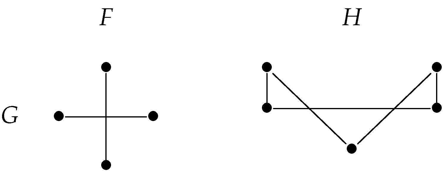
As an example, consider the situation in Figure 2. Although we are mainly interested in polygons, we will consider this simple example consisting of vertices and edges (and no faces). Hence, the intersection matrices are -matrices. Both configurations of points and line segments are topologically inconsistent, as in each case there are two line objects whose intersection is a point which is not an object of the configuration. The intersection matrices for the configurations, viewed as consisting of line segments, are
The configuration on the right of Figure 2 can be viewed as the boundary of a topologically inconsistent polygon. Another type of topologically inconsistent polygon is given when one vertex lies in the interior of an edge. Then, the intersection matrix of the boundary configuration is
depending on whether two edges intersect in their interiors or not.
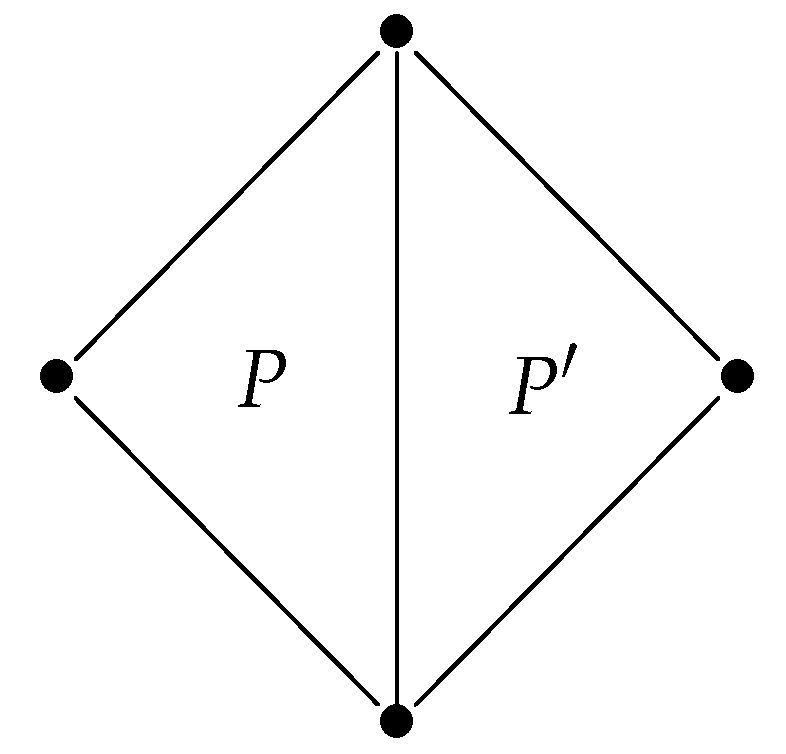
A topologically consistent configuration of two distinct triangles (this time with faces) is shown in Figure 3. The corresponding intersection matrix is the following -matrix:
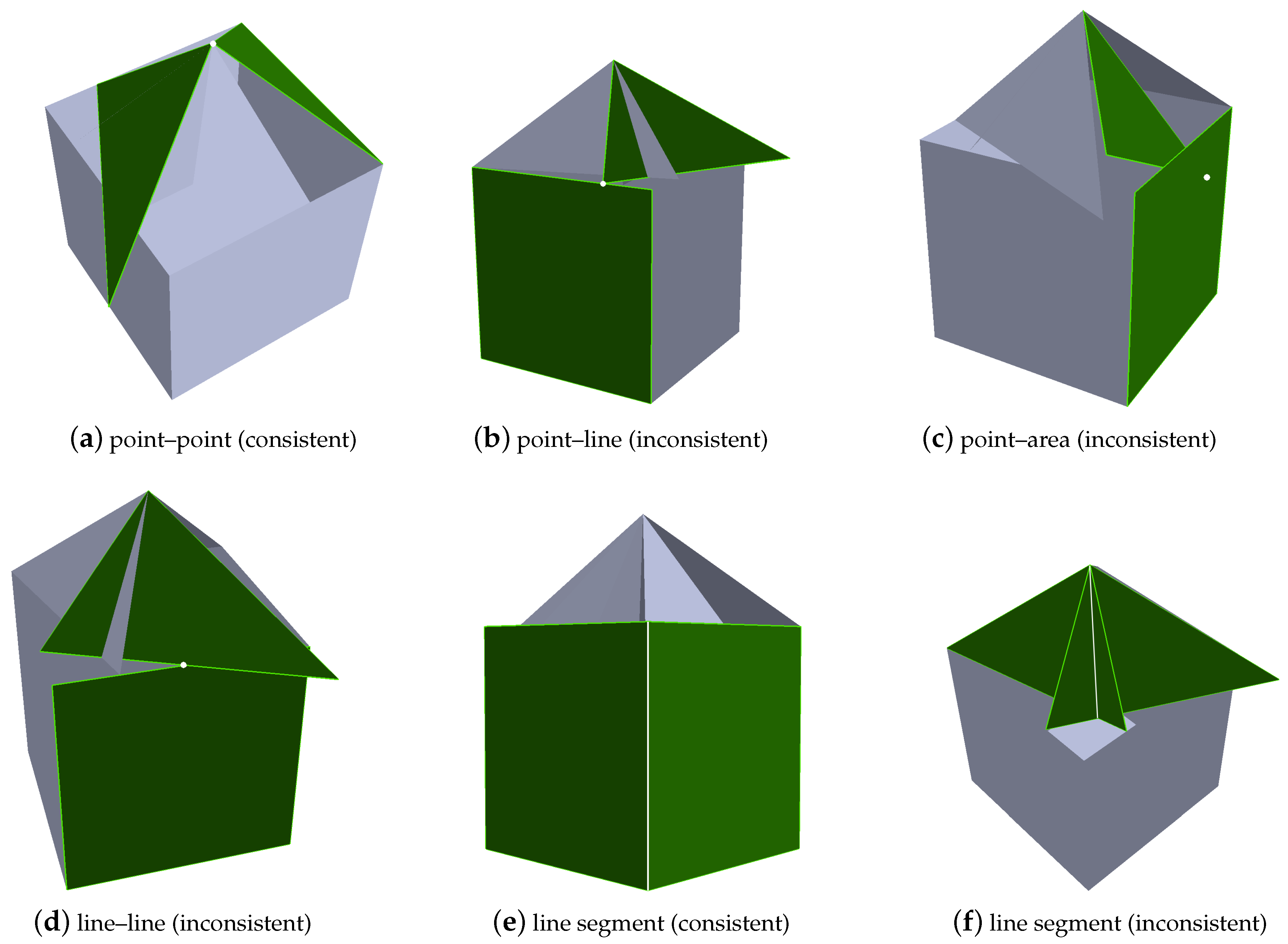
In Figure 4e, a three-dimensional constellation of two polygons is depicted that has the same corresponding intersection matrix.
2.5. Intersection Matrices of CityGML Data
CityGML has many different ways for defining entities in different contexts. However, in the case of surfaces in , the geometry used is that of polygons with holes by defining circular lists of coordinate triples (points in ) representing the vertices. From this information, it is possible to extract the vertices, edges and face of a polygon in order to compute intersection matrices. For example, it is possible to store the same configuration as a CompositeSurface or as a MultiSurface, although not all of the latter kind are allowed to be of the former kind, if the specifications of CityGML are followed correctly. We remark that, in this study, we do not check whether the data sets actually follow the specifications of CityGML correctly, we are only interested in extracting the cell posets of polygons in order to compute intersection matrices. Thus, the intersection matrix or the fact whether a polygon pair is topologically consistent or not does not depend on its (possibly incorrect) representation within a CityGML-file.
2.6. Diagonal Intersection Matrices
We will see below that, when intersecting two topologically consistent planar polygons P and in 3D, there are 54 ways in which the intersection matrix I can be populated. Of these, precisely four possible configurations can be topologically consistent. In these cases, I is a diagonal matrix:
Theorem 2.
If a configuration of two boundary representation geometries is topologically consistent, then its intersection matrix is a diagonal matrix.
Proof.
If the intersection matrix is not a diagonal matrix, this means that geometric objects of different dimensions intersect. This, however, means that Definition 1 is violated, i.e., the configuration is not topologically consistent. □
However, intersection matrix I being a diagonal matrix does not imply that the configuration is topologically consistent, as the following theorem shows.
Theorem 3.
Let a configuration of two planar polygons in be given, and let I be its intersection matrix. Then, the following statements hold true:
- 1.
- .
- 2.
- If or , then this configuration is topologically consistent.
- 3.
- If , , or , then this configuration is topologically inconsistent.
- 4.
- If or and P, lie in the same plane, then this configuration is topologically consistent. In the latter case, it follows that .
- 5.
- If or and P, do not lie in the same plane, then this configuration is topologically inconsistent.
Proof.
1. P and are closed subsets of . Hence, their intersection is also closed. However, if , then this intersection equals the non-empty intersection of the interiors of P and which is open in the connected space . However, the only subsets of which are closed and open are the empty set and the whole space . This cannot be.
2. In case , the intersection is empty. Hence, the configuration is topologically consistent. In case , the intersection is given by the intersection of vertices from P with vertices from . As distinct vertices cannot intersect, the configuration is topologically consistent.
3. Assume . In this case, only edge pairs have a non-empty intersection, and this must be a single point lying in their interiors. Hence, they cannot be the same edge.
Assume now, . This case is similar to the case , except that also the interiors of P and intersect. Again, all intersecting edge pairs must intersect in single points in their interiors, hence cannot be equal.
Assume finally that . In this case, the interiors of P and cannot coincide, as otherwise the two boundary curves must coincide. However, then also some edge has an intersection with some other boundary object.
In all three cases, it follows that the configuration is topologically inconsistent.
4. If or and P, lie in the same plane, then edges intersect other edges in whole edges or not at all. This suffices to see that the configuration is topologically consistent. In the latter case, it follows that .
5. If P and do not lie in the same plane, then line segments can intersect only in single points in their interiors. Hence, the configuration is topologically inconsistent. □
In [1], the intersection matrix is erroneously said to always come from a topologically consistent configuration of polygon pairs.
Theorem 4.
All diagonal matrices except occur as intersection matrices. The two ambiguous matrices according to Theorem 3 can be realised with topologically consistent as well as with topologically inconsistent configurations of polygon pairs in .
Proof.
Clearly, can be realised as an intersection matrix.
We have realised four diagonal intersection matrices in CityGML: realisations of inconsistent configurations modelled in CityGML with intersection matrices and are shown in Figure 4d,f. The topologically consistent configuration having the latter intersection matrix is given by .
Topologically consistent configurations with intersection matrices and are shown in Figure 4a,e.
In order to realise in a topologically inconsistent manner, let P be a polygon and a non-convex polygon with two vertices touching P in a vertex and a line, respectively.
The matrix can be realised as follows: let P and be squares having the same side length and not lying in the same plane. This configuration can be made such that the intersection of their interiors is a line segment without endpoints. These missing endpoints can be made to coincide with intersections of edges of P and by moving parallel to P along the direction of a pair of opposite edges of P.
The same method also realises : let the squares P and have two common vertices which are opposite to another in P as well as in . □
2.7. Intersection Matrices for Intersection Type Point
If the intersection of two polygons is a point, then there can occur four different intersection matrices. These four matrices can be given the following descriptive names:
As seen above, ‘point–point’ describes a topologically consistent, whereas ‘point–line’, ‘point–area’ and ‘line–line’ describe topologically inconsistent configurations of two distinct polygons. These four intersection constellations are depicted in Figure 4a–d, where you can see a simple synthetic example of a house with different kinds of topological inconsistencies.
2.8. Intersection Matrices for Arbitrary Polygon Pairs
Theorem 5.
Out of the symmetric -matrices with entries in , precisely 54 can occur as intersection matrices for pairs of planar polygons in .
Proof.
Let be planar polygons in . We can define as the -intersection matrix for the boundaries, as a -intersection matrix, and as a -intersection matrix. Now, we can define
where and
Clearly, if is a valid intersection matrix, then
and the supports of the three matrices are pairwise disjoint.
- First, observe that all possibilities for each of , , can be realised by pairs of planar polygons in , so their counts , respectively , are:
- Observe that any and any can be realised simultaneously. Namely, any can be realised in such a way that . In addition, if we want , then any exceptcan be realised with P and in the same plane. The latter intersection matrix can be realised with P and lying in non-parallel planes and with their interiors intersecting.
- Simultaneous realisation of and . The caseis the only one that needs special attention: In this case, the boundary points of any edge intersecting must have a non-empty intersection with the boundary of . This can be realised with in a common plane, or with in . In all other cases, all possible two values of are feasible.
- Simultaneous realisation of and . Ifthen two vertices of P lie in the boundary of . This means that the two matricesare impossible. However, all six of the others are realisable in this case. In all three other cases of , all eight possibilities for are realisable.
Summary. In total, there are 12 possibilities in case
and in all three of the other cases, there are possible realisations. Thus, all in all, there are
possible intersection matrices for planar polygons in . □
2.9. Implementation
From the previous subsections, we see that it was necessary to first calculate the intersection geometry (a geometric query), and then to check if the intersection is a union of common boundary objects (a topological query) for all pairs of polygons.
In order to make these topological and geometric queries, the CityGML data were imported into a 3D city database schema. 3DCityDB is a free Open Source package consisting of a database schema and a set of software tools to import, manage, analyse, visualise, and export virtual 3D city models according to the CityGML standard [30,31,32]. The database schema results from a mapping of the object oriented data model of CityGML 2.0 to the relational structure of a spatially-enhanced relational database management system (SRDBMS). The 3DCityDB supports the commercial SRDBMS Oracle (with ‘Spatial’ or ‘Locator’ license options) and the Open Source SRDBMS PostGIS which is an extension to the free RDBMS PostgreSQL and which was used for this work. 3DCityDB is in use in real-life production systems in many places around the world and is also being used in a number of research projects. As an example, consider [33]. According to [30], the cities of Berlin, Potsdam, Munich, Frankfurt, Zurich all keep and manage their virtual 3D city models within an instance of 3DCityDB. The included Importer/Exporter software tool allows for high performance importing and exporting of CityGML datasets according to CityGML versions 2.0 and 1.0. The tool allows the processing of very large datasets, even if they include XLinks between CityGML features or XLinks to three-dimensional GML geometry objects [34,35].
The implementation uses SFCGAL functions [36]. SFCGAL is a wrapper for the Computational Geometry Algorithms Library [37] that intends to implement 2D and 3D operations on OGC standard models (Simple Feature Access, CityGML, ...). Using the C API of SFCGAL, PostGIS exposes some of SFCGAL’s functions in spatial databases and can be patched for more functions.
The first part of the intersection analysis was done directly in the database using SQL queries, taking advantage of spatial indices. In order to effect this, the Procedural Language/PostgreSQL Structured Query Language (PL/pgSQL) [38] was used to write a function. PL/pgSQL was introduced to extend PostgreSQL’s SQL capabilities. For each intersecting pair of polygons, the intersection geometry was calculated and the geometry type of the intersection geometry was determined and the results were written into a newly created table in the database. For this purpose, corresponding SFCGAL functions were used, which are provided by PostGIS. PostGIS aims to support the SQL option of the OGC Simple Features Access standard [39]. Previously, all polygons were checked for validity, i.e., they were tested for planarity and self-intersection, and the position and orientation of interior rings were checked. For the validity check, the SFCGAL function isValid3d was used, which had to be patched to PostGIS, as the st_isValid function provided by PostGIS can only process two-dimensional geometries. The numerical uncertainties are defined by the default values used in SFCGAL functions st_isValid and st_3dintersects.
The intersection matrix operators were then implemented directly in C++ within the SFCGAL framework, since the SFCGAL functions provided by PostGIS were not sufficient to perform the necessary queries directly on the database. For this purpose, the pairs of polygons whose intersection geometry type is Point or a line segment (i.e., LineString consisting of only two points) were first exported from the database, and then further processed by a C++ function. For now, only these two types of intersection geometries have been considered, as they occur most often in CityGML datasets and it is quite easy for them to determine the intersection constellation. If the intersection geometry is a point, then, as described in Section 2.4, there are four possible intersection matrices, of which exactly one comes from a topologically consistent configuration. To determine the intersection matrix, it is first checked if the point of intersection is equal to one of the vertices of one or both of the intersected polygons. If a matching vertex is found on both polygons, it means that both polygons intersect at that point. For this configuration, the intersection matrix corresponds to ’point–point’. This case is topologically consistent. If no matching vertex is found on either of the two polygons, then the intersection matrix corresponds to ’line–line’, as this is only possible when two edges of the polygons intersect. If the intersection point is identical to a vertex of one of the two intersected polygons, then it is further tested whether it lies on one edge of or inside the other polygon. If it lies on one edge of the other polygon, then the intersection matrix corresponds to ’point–line’ and if it lies within the interior of the other polygon, the intersection matrix corresponds to ’point–area’.
For the intersection geometry type line segment, a distinction was made only between consistent and inconsistent, since it would be very costly to determine the exact intersection matrices for all possible configurations. In fact, the set of all possible configurations of two distinct polygons for a given intersection matrix has not yet been found, except in the case when the intersection is a point. To distinguish between consistent and inconsistent intersection constellations of a line segment, it is sufficient to check if both polygons contain the intersection geometry, i.e., whether the line segment is identical to an edge of both polygons. If so, the configuration is topologically consistent; otherwise, it is inconsistent.
3. Results
For this study, real-world CityGML data sets were used as shown in Table 1. The largest data set contains the whole city of Berlin in LoD2. This data set was generated from extracted cadastral data. The CityGML files were downloaded from [40]. The data set can be viewed via links provided on the Github page of the 3dcitydb-web-map project [41]. In addition, five data sets from Karlsruhe were examined. These data sets come from the “Liegenschaftsamt” of the city of Karlsruhe. Four of them contain single streets or small residential areas of the city of Karlsruhe, which were generated from LIDAR data and modelled in LoD2. The data set “Karlsruhe KIT/CS” covers an area of 1.73 × 1.14 km. Its layout can be seen in Figure 8. The two other real-world data sets are available in LoD1. These are the whole city of Potsdam and the village Waldbrücke, which is part of the municipality Weingarten near Karlsruhe. The Potsdam data set is included in the download package of the 3DCityDB and Waldbrücke was downloaded from the CityGML homepage.
Table 1 shows a list of the CityGML data sets used in this study together with the number of polygons and non-empty intersections of distinct polygons. The column “valid polygons” gives the proportion of valid polygons within the data set as imported into a 3DCityDB database. Column “intersections” gives the total number of all non-empty intersections made with valid polygons. The columns “inconsistent buildings” give the proportion of buildings containing invalid polygons or a topologically inconsistent point or line segment intersection, or an intersection of types TIN (Triangulated Irregular Network) or Triangle. In addition, “val3dity” gives the proportion of buildings containing invalid solids according to val3dity. Notice that the number of non-empty intersections captures all polygons from the whole data set, even if they belong to different buildings. Thus, if, e.g., two individual buildings in one data set are not found to have topologically inconsistent pairs of polygons, it may happen that there is a pair in the union of the two buildings which is topologically inconsistent. In fact, our method is to check any given pair of polygons for topological (in)consistency, without taking any other properties into account, like the buildings they belong to.
It can be seen that, for all data sets except Berlin, the vast majority of polygons are valid, i.e., are both planar and without self-intersections and if there exists an interior ring, its position and orientation are correct. In particular, they are topologically consistent. The values may differ from previous results given in [1] because this time all CityGML objects were imported into the databases instead of just importing the buildings.
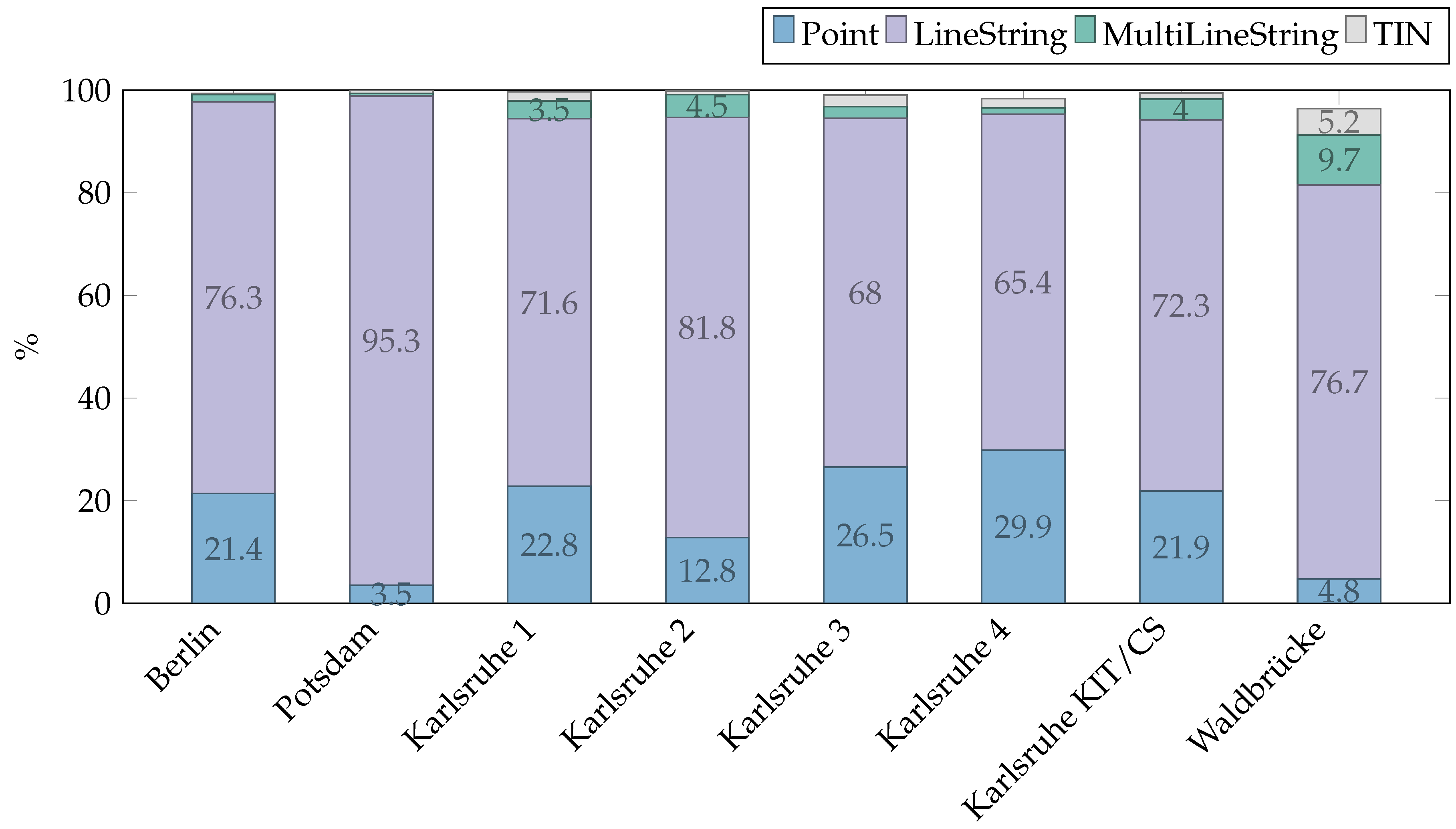
Figure 5 shows the percentages of polygon intersection types when the intersection is non-empty and the two polygons are distinct. A MultiLineString is a union of LineStrings with at least two components. TIN stands for Triangulated Irregular Network and means that the configuration is topologically inconsistent, as the intersection contains a surface strictly contained in the faces of both polygons. The other types may or may not be topologically consistent. It can be seen that the intersection is, in the vast majority of instances, either a point or a line segment. This is the reason why these two types of intersections were further investigated. In addition, the data sets from Karlsruhe have a high proportion of intersections of the type Point.
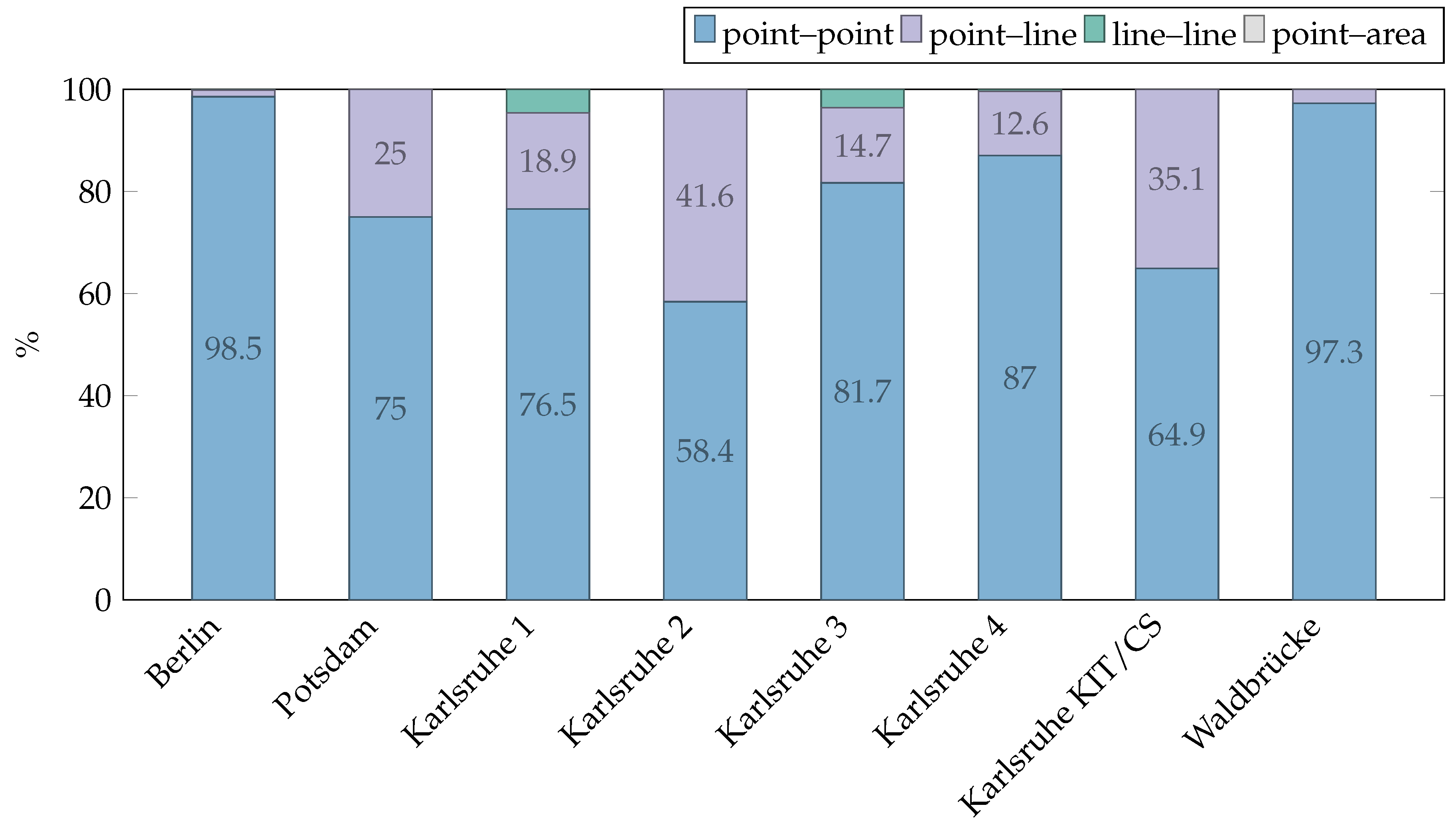
Figure 6 shows the relative frequencies of occurrences of the four intersection matrices when the intersection of two distinct polygons is a point. The majority consists of the topological consistent case of ‘point–point’. However, most data sets have a large proportion of topologically inconsistent intersection matrices of type ‘point–line’.
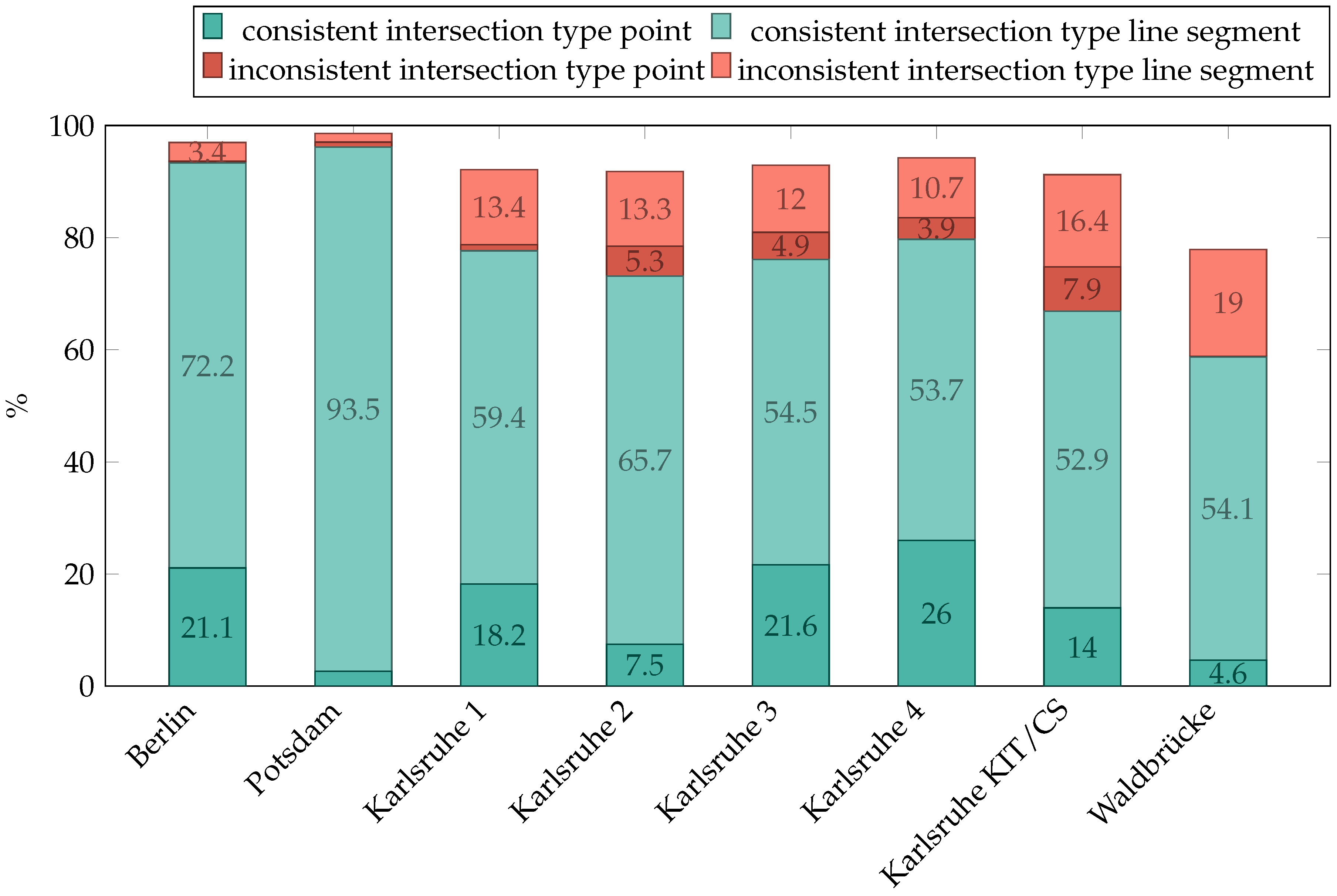
Figure 7 shows the proportion of topologically consistent or inconsistent polygon pairs when the intersection is a point or a line segment (special case of the type LineString). These are by far the most frequent intersection types.
4. Discussion
The results show that there is a high inhomogeneity between the data sets. The distribution of the intersection types and the proportion of topologically inconsistent constellations seem to depend on the type of data collection and the Level of Detail.
In [16], a tool is described named val3dity for validating solids against the ISO/OGC specifications defined in CityGML and various other 3D data formats. This tool also checks if pairs of distinct solids intersect in their interiors. However, it does not verify if they intersect in a topologically inconsistent way in their boundaries, as seen in Corollary 1. This would necessitate the check of intersecting polygon pairs. Different to val3dity, the aim of this work here is to check topological consistency regardless of the conformity to the corresponding standards. For example, the topologically inconsistent example house used here for illustration purposes has been run through val3dity and has been found ‘valid’, when it is modelled as a combination of MultiSurfaces, which is correct according to the CityGML standard. The comparison of val3dity to our methodology is only possible if building shells are modelled as Solid, which means one exterior shell minus possible interior shells. The assignment of polygons to buildings becomes problematic if the building shell is modelled as MultiSurface geometries instead of Solid. For this reason, buildings with inconsistent polygons and polygon pairs can only be determined in case they are modelled as Solid (cf. Table 1). Notice that our approach is to check any polygon pair which potentially has a non-intersection without regarding any non-geometric properties like the building they belong to. In this way, e.g., inconsistencies between buildings which are consistent themselves could be found.
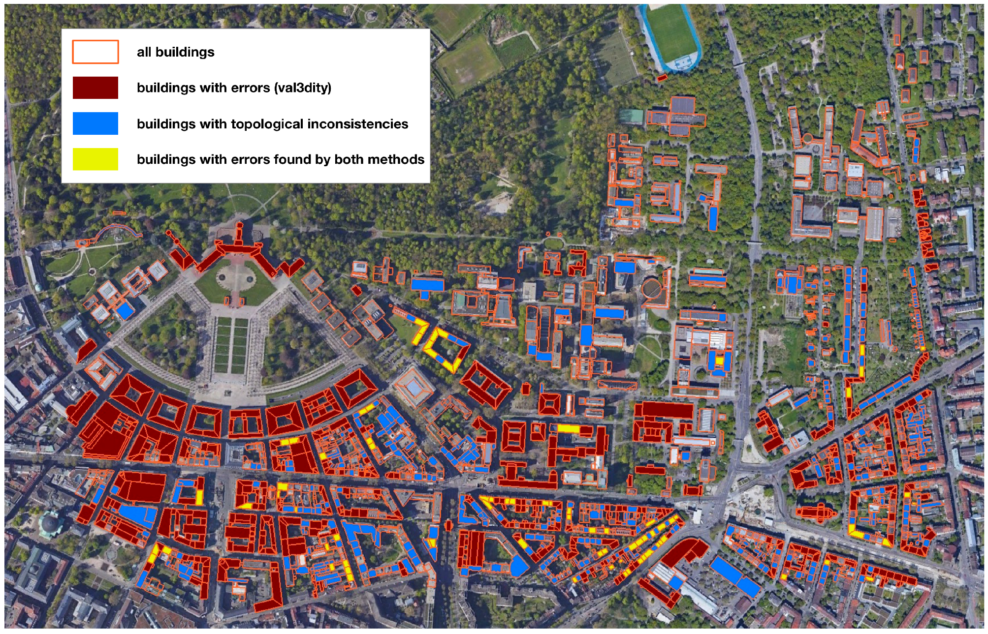
For the data sets “Berlin” and “Karlsruhe KIT/CS”, the inconsistent buildings found by our topological analysis and those found by val3dity (version 2.1.1) have been compared by their identifiers. Due to the differing definitions of error or inconsistency, the overlap is relatively small. In the “Berlin” data set, we have identified 6392 distinct buildings with inconsistencies in the database. For the analysis with val3dity, we have exported the whole database as one CityGML file. In addition, 723 inconsistent buildings have been identified by val3dity this way. Both sets of resulting building identifiers have an overlap of 113 identical building identifiers found by both methods. In the “Karlsruhe KIT/CS” data set, we found 497 inconsistent buildings, and val3dity found 319 with 78 buildings being in both sets (cf. Figure 8).
In [42], the most common geometric and semantic errors in CityGML data are analysed. They find that the most common topological errors are that polygons are not properly oriented, and that geometries are not properly “snapped”. From what is stated there, one can see that our approach is, on the one hand, a further differentiation of that error type, and, on the other hand (unlike loc. cit.), we do not require a building to consist of solids only, as long as the polygons intersect in common boundary elements, e.g., balconies, porches, and shelters often have geometries which do not form a shell, i.e., are non-closed surfaces.
5. Conclusions
The aim of boundary representation models is to represent the topology underlying geometric models. However, in order to correctly represent the topology, the correctness of the incidence graph of the B-Rep model is needed. This is only the case if the topology underlying the geometric model coincides with the topology underlying the B-Rep model—in other words, if the data are topologically consistent in our sense. In the case of CityGML, it is possible to model correctly according to the standard and still have a topologically inconsistent model. A consequence is that CityGML does not comply with the ISO 19107 standard.
Towards distinguishing between different forms of topological inconsistency, the intersection matrix defined here is a first indicator. However, some matrices are ambiguous: they can come from both consistent and inconsistent configurations. A classification of these matrices has been done. In particular, it has been shown which matrices can occur as intersection matrices, and that intersection matrices of topologically consistent data are diagonal matrices.
The results show that many buildings modelled in CityGML contain a large number of polygon pairs forming a topologically inconsistent configuration. Some of these buildings pass through the test of val3dity, which often found other kinds of errors in the buildings studied for this article. The fact that the observed overlap between our method and val3dity is very small shows that the notion of topological consistency considered here complements the plethora of consistency definitions for topological models of geographical objects. The one considered here relates geometry and the incidence graph in a way that the topology of the underlying geometric model must coincide with the topology from the incidence graph. In the case of the buildings under study, the distribution of their inconsistency types varies, the most frequent inconsistent case being when the intersection of two polygons is a line segment. When the intersection is a point, the most frequent inconsistency is given by a vertex lying in the interior of a line segment. As efficient topological queries rely on the correctness of the incidence graph, it follows that the data studied here are not suitable for analysis which goes beyond mere visualisation. Consequently, when producing a geometry model in CityGML from point cloud data, it is necessary to include a check for topological consistency in the sense of this article. Furthermore, a desideratum is to find ways of healing topological inconsistent data, possibly depending on the type of topological inconsistencies encountered.
Author Contributions
The authors jointly contributed to the concept of this paper, the discussion of derived results, and the writing of the paper. The implementation of the framework and the evaluation of the framework on CityGML data sets were done by Anna Giovanella and Sven Wursthorn.
Funding
This research was partially funded by the Deutsche Forschungsgemeinschaft under Grant No. BR 3513/12-1.
Acknowledgments
We acknowledge support by the Deutsche Forschungsgemeinschaft and Open Access Publishing Fund of the Karlsruhe Institute of Technology. The Liegenschaftsamt of the City of Karlsruhe is thanked for data sets. The anonymous referees are thanked for valuable criticism which led to corrections of errors and to a better exposition of the contents of this article. In particular, one referee contributed to the insight that the ISO 19107 standard is equivalent to our notion of topological consistency for configurations as defined in this article.
Conflicts of Interest
The authors declare no conflict of interest.
References
- Giovanella, A.; Bradley, P.E.; Wursthorn, S. Detection and evaluation of topological consistency in CityGML datasets. ISPRS Ann. Photogramm. Remote Sens. Spat. Inf. Sci. 2018, 4, 59–66. [Google Scholar] [CrossRef]
- Biljecki, F.; Stoter, J.; Ledoux, H.; Zlatanova, S.; Çöltekin, A. Applications of 3D City Models: State of the Art Review. ISPRS Int. J. Geo-Inf. 2015, 4, 2842–2889. [Google Scholar] [CrossRef] [Green Version]
- Bradley, P.; Paul, N. Using the relational model to capture topological information of spaces. Comput. J. 2010, 53, 69–89. [Google Scholar] [CrossRef]
- Paul, N. Topologische Datenbanken für Architektonische Räume. Ph.D. Thesis, Universität Karlsruhe, Karlsruhe, Germany, 2008. [Google Scholar]
- Joksić, D.; Bajat, B. Elements of spatial data quality as information technology support for sustainable development planning. Spatium 2004, 11, 77–83. [Google Scholar] [CrossRef]
- Li, S. On topological consistency and realization. Constraints 2006, 11, 3151. [Google Scholar] [CrossRef]
- Kang, H.; Li, K. Assessing topological consistency for collapse operation in generalization of spatial databases. In Perspectives in Conceptual Modeling; Akoka, J., Ed.; Lecture Notes in Computer Science; Springer: Berlin/Heidelberg, Germany, 2005; Volume Voume 3770. [Google Scholar]
- Rodriguez, M.; Brisaboa, N.; Meza, J.; Luaces, M. Measuring consistency with respect to topological dependency constraints. In Proceedings of the 18th SIGSPATIAL International Conference on Advances in Geographic Information Systems, San Jose, CA, USA, 3–5 November 2010; pp. 182–191. [Google Scholar]
- Bradley, P. Supporting Data Analytics for Smart Cities: An Overview of Data Models and Topology. In Statistical Learning and Data Sciences SLDS 2015; Gammerman, A., Vovk, V., Papadopoulos, H., Eds.; Lecture Notes in Computer Science; Springer: Cham, Switzerland, 2015; Volume 9047, pp. 406–413. [Google Scholar]
- Jahn, M.; Bradley, P.; Al-Doori, M.; Breunig, M. Topologically consistent models for efficient big geo-spatio-temporal data distribution. ISPRS Ann. Photogramm. Remote Sens. Spat. Inf. Sci. 2017, IV-4/W5, 65–72. [Google Scholar] [CrossRef]
- Alam, N.; Wagner, D.; Wewetzer, M.; von Falkenhausen, J.; Coors, V.; Pries, M. Towards Automatic Validation and Healing of CityGML Models for Geometric and Semantic Consistency. In Innovations in 3D Geo–Information Sciences; Isikdag, U., Ed.; Springer International Publishing: Cham, Switzerland, 2014; pp. 77–91. [Google Scholar]
- Gröger, G.; Plümer, L. How to Achieve Consistency for 3D City Models. Geoinformatica 2011, 15, 137–165. [Google Scholar] [CrossRef]
- Ledoux, H.; Meijers, M. Topologically consistent 3D city models obtained by extrusion. Int. J. Geogr. Inf. Sci. 2011, 25, 557–574. [Google Scholar] [CrossRef] [Green Version]
- Biljecki, F.; Ledoux, H.; Stoter, J. Improving the Consistency of Multi-LOD CityGML Datasets by Removing Redundancy. In 3D Geoinformation Science: The Selected Papers of the 3D GeoInfo 2014; Breunig, M., Al-Doori, M., Butwilowski, E., Kuper, P.V., Benner, J., Haefele, K.H., Eds.; Lecture Notes in Geoinformation and Cartography; Springer International Publishing: Cham, Switzerland, 2015; pp. 1–17. [Google Scholar]
- Steuer, H.; Machl, T.; Sindram, M.; Liebel, L.; Kolbe, T. Voluminator—Approximating the Volume of 3D Buildings to Overcome Topological Errors. In AGILE 2015; Bacao, F., Santos, M., Painho, M., Eds.; Lecture Notes in Geoinformation and Cartography; Springer: Cham, Switzerland, 2015. [Google Scholar]
- Ledoux, H. val3dity: Validation of 3D GIS primitives according to the international standards. Open Geospat. Data Softw. Stand. 2018, 3, 1. [Google Scholar] [CrossRef]
- Gröger, G.; Plümer, L. CityGML—Interoperable semantic 3D city models. ISPRS J. Photogramm. Remote Sens. 2012, 71, 12–33. [Google Scholar] [CrossRef]
- Gröger, G.; Kolbe, T.H.; Nagel, C.; Häfele, K.H. OGC City Geography Markup Language (CityGML) Encoding Standard; Open Geospatial Consortium: Wayland, MA, USA, 2012. [Google Scholar]
- Cox, S.; Daisey, P.; Lake, R.; Portele, C.; Whiteside, A. Geography Markup Language (GML) Encoding Specification; Open Geospatial Consortium: Wayland, MA, USA, 2002. [Google Scholar]
- Foley, J.D.; van Dam, A.; Feiner, S.K.; Hughes, J.F. Computer Graphics: Principles and Practice in C, 2nd ed.; Addison–Wesley Professional: Boston, MA, USA, 1996. [Google Scholar]
- Hatcher, A. Algebraic Topology; Cambridge University Press: Cambridge, MA, USA, 2002. [Google Scholar]
- Alexandrov, P. Diskrete Räume. Matematicheskii Sbornik (N.S.) 1937, 2, 501–518. [Google Scholar]
- Barmak, J. Algebraic Topology of Finite Topological Spaces and Applications; Lecture Notes in Mathematics; Springer: Cham, Switzerland, 2011; Volume 2032. [Google Scholar]
- Jähnich, K. Topology; Undergraduate Texts in Mathematics; Springer: New York, NY, USA, 1984. [Google Scholar]
- Björner, A. Posets, Regular CW Complexes and Bruhat Order. Eur. J. Comb. 1984, 5, 7–16. [Google Scholar] [CrossRef] [Green Version]
- Bradley, P.; Paul, N. Topologically Consistent Space, Time, Version, and Scale Using Alexandrov Topologies. In Contemporary Strategies and Approaches in 3D, Information Modeling; Kumar, B., Ed.; IGI Global: Hershey, PA, USA, 2018; pp. 52–82. [Google Scholar]
- ISO/TC 211. ISO 19107:2003 Geographic Information—Spatial Schema. 2003. Available online: https://www.iso.org/obp/ui/#iso:std:iso:19107:ed-1:v1:en (accessed on 3 June 2019).
- Egenhofer, M.J. Reasoning about binary topological relations. In Advances in Spatial Databases; Günther, O., Schek, H.J., Eds.; Springer: Berlin/Heidelberg, Germany, 1991; pp. 141–160. [Google Scholar]
- Giovanella, A. Automatische Redundanzfreie Generierung von Topologie aus Multidimensionalen Geographischen Datenbeständen. Ph.D. Thesis. in progress.
- 3DCityDB. 3DCityDB Database Schema for CityGML. 2018. Available online: https://www.3dcitydb.org/3dcitydb/3dcitydbhomepage/ (accessed on 25 April 2018).
- Stadler, A.; Nagel, C.; König, G.; Kolbe, T. Making interoperability persistent: A 3D geo database based on CityGML. In 3D Geo–Information Sciences; Lee, J., Zlatanova, S., Eds.; Lecture Notes in Geoinformation and Cartography; Springer: Berlin/Heidelberg, Germany, 2009; Chapter 11; pp. 175–192. [Google Scholar]
- Yao, Z.; Nagel, C.; Kunde, F.; Hudra, G.; Willkomm, P.; Donaubauer, A.; Adolphi, T.; Kolbe, T.H. 3DCityDB—A 3D geodatabase solution for the management, analysis, and visualization of semantic 3D city models based on CityGML. Open Geospat. Data Softw. Stand. 2018, 3, 5. [Google Scholar] [CrossRef]
- Chaturvedi, K.; Yao, Z.; Kolbe, T. Web-based Exploration of and Interaction with Large and Deeply Structured Semantic 3D City Models using HTML5 and WebGL. In 35. Wissenschaftlich–Technische Jahrestagung der DGPF; Deutsche Gesellschaft für Photogrammetrie, Fernerkundung und Geoinformation e.V.: München, Germany, 2015. [Google Scholar]
- Kunde, F. CityGML in PostGIS—Portierung, Anwendung und Performanz–Analyse am Beispiel der 3DCityDB Berlin. Master’s Thesis, Universität Potsdam, Potsdam, Germany, 2012. [Google Scholar]
- Kunde, F.; Nagel, C.; Herrerruela, J.; Ross, L.; Kolbe, T.H. 3D-Stadtmodelle in PostGIS mit der 3D City Database. Proceedings of Tagungsband der FOSSGIS-Konferenz, Rapperswil, Switzerland, 12–14 June 2013. [Google Scholar]
- SFCGAL. Simple Features Wrapper Library for CGAL. 2018. Available online: http://www.sfcgal.org (accessed on 25 April 2018).
- CGAL. Computational Geometry Algorithms Library. 2018. Available online: http://www.cgal.org/ (accessed on 25 April 2018).
- Eisentraut, P. PostgreSQL: Das offizielle Handbuch; Verlag Moderne Industrie: Landsberg am Lech, Germany, 2003. [Google Scholar]
- Herring, J.R. OpenGIS® Implementation Standard for Geographic Information—Simple Feature Access—Part 2: SQL Option; Technical Report OGC 06-104r4; Open Geospatial Consortium Inc.: Wayland, MA, USA, 2010. [Google Scholar]
- Berlin Business Location Center. Berlin 3D—Download Portal. 2018. Available online: http://www.businesslocationcenter.de/en/downloadportal (accessed on 29 April 2018).
- Chair of Geoinformatics, Technical University of Munich. Cesium-Based 3D Viewer and JavaScript API for the 3D City Database. 2019. Available online: https://github.com/3dcitydb/3dcitydb-web-map (accessed on 30 April 2018).
- Biljecki, F.; Ledoux, H.; Du, X.; Stoter, J.; Soon, K.H.; Khoo, V.H.S. The most common geometric and semantic errors in CityGML datasets. ISPRS Ann. Photogramm. Remote Sens. Spat. Inf. Sci. 2016, IV-2/W1, 13–22. [Google Scholar] [CrossRef]
Figure 1.
A topologically consistent configuration given as a partitioned space K (left) and its face poset (right).
Figure 1.
A topologically consistent configuration given as a partitioned space K (left) and its face poset (right).

Figure 2.
Two topologically inconsistent situations.

Figure 3.
A topologically consistent configuration of two distinct triangles G (left) and (right).

Figure 4.
Simple synthetic example of a house with different kinds of topological inconsistencies. The green geometries depict the different types of intersection constellations.
Figure 4.
Simple synthetic example of a house with different kinds of topological inconsistencies. The green geometries depict the different types of intersection constellations.

Figure 5.
Proportions of the most frequent non-empty polygon intersection types.

Figure 6.
Intersection matrices when intersection is a point.

Figure 7.
Topologically consistent and inconsistent configurations with point and line segment intersections.
Figure 7.
Topologically consistent and inconsistent configurations with point and line segment intersections.

Figure 8.
Building layout of the “Karlsruhe KIT/CS” data set with topologically inconsistent buildings found by both methods. Background layer: ©2019 Google, CityGML data: ©City of Karlsruhe, Liegenschaftsamt, 2019.
Figure 8.
Building layout of the “Karlsruhe KIT/CS” data set with topologically inconsistent buildings found by both methods. Background layer: ©2019 Google, CityGML data: ©City of Karlsruhe, Liegenschaftsamt, 2019.


Table 1.
List of CityGML data sets used in this study.
| Valid | Number of | Number of | Inconsistent Buildings | ||
|---|---|---|---|---|---|
| Data Set Name | Polygons [%] | Intersections | Buildings | [%] | Val3dity [%] |
| Berlin | 35.1 | 511,204 | 51,211 | 12.5 | 1.4 |
| Potsdam | 100.0 | 9074 | 97 | 22.7 | 0.0 |
| Karlsruhe 1 | 86.7 | 4564 | 95 | 84.2 | 0.0 |
| Karlsruhe 2 | 92.5 | 3530 | 67 | 55.2 | 7.5 |
| Karlsruhe 3 | 90.4 | 4410 | 64 | 51.6 | 0.0 |
| Karlsruhe 4 | 80.8 | 5066 | 104 | 68.3 | 1.9 |
| Karlsruhe KIT/CS | 87.8 | 430,384 | 1125 | 44.2 | 19.1 |
| Waldbrücke | 93.6 | 20,644 | 491 | 4.3 | 1.4 |
© 2019 by the authors. Licensee MDPI, Basel, Switzerland. This article is an open access article distributed under the terms and conditions of the Creative Commons Attribution (CC BY) license (http://creativecommons.org/licenses/by/4.0/).
Share and Cite
MDPI and ACS Style
Giovanella, A.; Bradley, P.E.; Wursthorn, S. Evaluation of Topological Consistency in CityGML. ISPRS Int. J. Geo-Inf. 2019, 8, 278. https://0-doi-org.brum.beds.ac.uk/10.3390/ijgi8060278
AMA Style
Giovanella A, Bradley PE, Wursthorn S. Evaluation of Topological Consistency in CityGML. ISPRS International Journal of Geo-Information. 2019; 8(6):278. https://0-doi-org.brum.beds.ac.uk/10.3390/ijgi8060278
Chicago/Turabian StyleGiovanella, Anna, Patrick Erik Bradley, and Sven Wursthorn. 2019. "Evaluation of Topological Consistency in CityGML" ISPRS International Journal of Geo-Information 8, no. 6: 278. https://0-doi-org.brum.beds.ac.uk/10.3390/ijgi8060278
Note that from the first issue of 2016, this journal uses article numbers instead of page numbers. See further details here.