Article

Impact of a Vicinity of Airport on the Prices of Single-Family Houses with the Use of Geospatial Analysis

by
Radosław Cellmer
1,
Mirosław Bełej
1,* and
Jan Konowalczuk
2
1
Institute of Geospatial Engineering and Real Estate, University of Warmia and Mazury in Olsztyn, Prawocheńskiego 15, 10-720 Olsztyn, Poland
2
Department of Real Estate Economics and Investment, Cracow University of Economics, ul.Rakowiecka 27, 31-510 Krakow, Poland
*
Author to whom correspondence should be addressed.
ISPRS Int. J. Geo-Inf. 2019, 8(11), 471; https://0-doi-org.brum.beds.ac.uk/10.3390/ijgi8110471
Submission received: 3 September 2019 / Revised: 2 October 2019 / Accepted: 19 October 2019 / Published: 23 October 2019
(This article belongs to the Special Issue Applications of GIScience for Land Administration)

Abstract

:
This article analyses the adverse impact of Chopin Airport in Warsaw on the prices of single-family houses located within the aircraft noise impact zone. The specific feature of the largest airport in Poland is its location within the city limits and the resulting direct surroundings of both multi- and single-family housing developments. Not only is the nuisance due to the proximity of the airport resulting from the actual exposure to an excessive noise level but also from legal restrictions associated with the Limited Use Area (LUA). The study used statistical modeling by applying a classic multiple regression model, spatial autoregressive model and geographically weighted regression model. Moreover, Geographical Information System (GIS) tools and geostatic modeling were used to visualise the results. The modeling results clearly show the significant impact of the neighborhood nuisance and the related spatial distribution of real estate prices. In addition, the geographically weighted regression model indicates that the proximity to an airport adversely affects the rate of price changes over time.

1. Introduction

Airports and aviation make up an important contribution to local, regional and state economies. The influence on local and regional economic activity extends well beyond the airport site. The location of airports influences the geographic distribution of industries and can be a significant factor in the decisions of certain industries to locate in a specific province or region [1]. In urbanised areas, airports are the specific centres of the local transport infrastructure that determines significant intensification of the road and rail infrastructure network. The specific nature of air traffic necessitates efficient transport, particularly public transport (buses, trams, local railway) from the urban area or region to the airport zone. This results in an increase in the investment attractiveness of the areas located in the vicinity of the airport, both in terms of commercial and residential investments. The literature on the subject mentions many positive effects of an airport’s impact on the community and economic development, including an increase in employment [2], an increase in the local community income [3], an increase in infrastructural amenities for the local community [1], an increase in local business innovativeness [4], and an increase in the tourism traffic volume [5].
Apart from the undoubted benefits of the sustainable development of society, airports and aviation also generate some general (social and economic) costs. There is no doubt that an increase in the level of aircraft noise is, and will continue to be, an increasingly serious problem for people living in the vicinity of airports (both large international airports and less important local ones). Three factors influence noise burden: the number of flights, the level of noise emitted by each airplane and the time of flight [6]. In many cases, there is a strong tension between economic sustainability (long-term economic growth, stable employment, infrastructure development), and environmental sustainability (limitation of negative externalities—noise, pollution) of the airport’s operation. As a consequence, airport growth influences local planning and is often converted into restrictive local zoning plans, limiting potential development on the affected area in order to eliminate negative externalities [7]. Therefore, the establishment or enlargement of an airport always results in the occurrence of nuisance associated with its proximity, and the inability to meet the environmental protection standards related to noise. According to Polish regulations, where the results of the environmental impact assessment proceedings provide evidence indicating that despite the application of technical, technological and organisational solutions in airports, environmental quality standards cannot be met, a so-called limited use area (LUA) needs to be established. Although the introduction of such an area in the immediate vicinity of an airport limits the possibility for using real estate (principles of land development and its uses), it supports the owners in obtaining compensation for these limitations (and the necessity to withstand the exceeded noise standards), as well as provides an opportunity to obtain financial resources for the acoustic upgrading of their houses.
The article makes an attempt to determine the impact of Poland’s Warsaw Chopin Airport’s adverse effects on the prices of single-family houses located within the limited use zone and in close proximity outside this zone. Therefore, the main aim of the study is to determine, using statistical modeling, the differences in prices between real estate located within the LUA and outside this zone.

2. Theoretical Basic of Conducted Research

The assessment of the adverse impact of airports on the housing market has been the subject of numerous scientific studies using a number of research methods. The relationship between the housing prices and the proximity of the Paris–Charles-de-Gaulle (CDG) airport was the subject of research conducted by [8]. The negative impact on the price of real estate has been analysed by applying a hedonic pricing method and evaluating the consequences in terms of environmental inequalities and social justice. Moreover, this article draws attention to the increase in population density in the Noise Exposure Plans (NEP) areas despite the increased noise levels and the limitations of the uses of these areas. The hedonic price method was also used to find a statistically significant negative relationship between residential real estate values and airport noise and the proximity to the airport in the Reno–Sparks area [9,10]. Trojanek R. et al. [6] analysed the impact of aircraft noise on housing prices using the hedonic method and the OLS (ordinary least squares), WLS (weighted least squares), SAR (spatial autoregressive model) and SEM (spatial error model) models.
The fundamental issue from the perspective of this study is the analysis referring to the selection of the appropriate form of a model describing the relationships occurring in the housing market, including in particular the relationship between the real estate features and prices. As a general rule, studies into the relationships in housing markets are carried out through the application of the multiple linear regression model [11]. The classic form of the multiple linear regression model can be described using the following formula:
y = β X + ε
where:
  • y—is a response variable,
  • β—is a vector of coefficients (model parameters),
  • X—is a matrix of explanatory variables,
  • ε—is a vector of random components of the model.
Classic regressive models applied for the analysis of the real estate market usually do not directly consider the potential interactions (spatial autocorrelation), which may occur between the level of a particular phenomenon in the space, and assume the stability of the process (spatial homogeneity) associated with the development of prices within the geographical space. Spatial autocorrelation refers to the occurrence of interdependencies between observations in the geographical space, while heterogeneity refers to the general, systematic variability in the preservation of a particular process within the entire space. In the spatial econometrics’ literature, the negative consequences of ignoring the presence of spatial autocorrelation and/or spatial heterogeneity are well known, hence numerous publications on market analysis and price prediction propose the application of spatial models [12,13]. Spatial effects can be taken into account in many ways, i.e., by applying the spatial econometric model [14], spatially switching regression [15], random coefficient models [16], semi-logarithmic model using a row-standardized distance based spatial weight matrix [17], or geographically weighted regression [18].
This article applied the spatial autoregressive (SAR) model and the geographically weighted regression (GWR) model, in addition to the application of a classical multiple regression model for the assessment of the impact of the Warsaw Chopin Airport’s effects on the prices of single-family houses.
Spatial regressive models are applied in situations when real estate prices or the remainders of transaction price regressive models are spatially correlated. The application of spatial regression models [13,19] is particularly justified in a situation when transaction prices are affected by continuous factors that characterise the condition of the environment (air pollution, noise, the level of urban greenery saturation). Detailed principles concerning the construction and testing of spatial autoregressive models are provided by Anselin L. [15] and Arbia G. [20], among others. Besner C. [21] demonstrated that the application of autoregressive models significantly improved the prediction accuracy. A general form of models considering spatial lag, also referred to as spatial autoregressive models (SAR), is as follows:
y = ρ W y + X β + ε
where:
  • X—is a matrix of explanatory variables,
  • β—is a vector of coefficients (model parameters),
  • ε ~ ~N(0,σ2I) is a vector of model errors,
  • Wy—is defined as a spatially lagged response variable and
  • ρ—is a spatial autocorrelation coefficient.
The basis for the application of geographically weighted regression is an assumption that model parameters can be estimated separately at each point of the space for which the values of the response variable and explanatory variables are known. Interactions occurring between tested objects in space are, in many cases, characterised by the fact that the elements located nearby most frequently have more similarities than the objects that are far from each other. The application of this principle enables an estimation of the model parameters in a particular location, on the assumption that the observations made at points located closer to the point under study will have a correspondingly greater weight than the observations located at a further distance [22]. Geographically weighted regression according to [23] should be used as a method for exploring spatial nonstationarity. The equation of a typical GWR model will take the following form:
Y = β 0 ( x i , y i ) + β 1 ( x i , y i ) X + ε i
or, for multiple explanatory variables:
Y = β 0 ( x i , y i ) + j = 1 k β j ( x i , y i ) X j + ε i ,   for   i = 1 , 2 ,   n
where the value of model parameters is related to the location, in this case expressed by coordinates (xi, yi). Hence, β0 is the constant of the model, βj is a regression coefficient for the j-th variable, while εi is a random error of the model in a location with coordinates (xi, yi). Geographically weighted regression is widely used to analyse the spatial dynamics of real estate prices. Among other things, in the paper [24] GWR model has been adopted for analyzing the housing market in the city of Potenza (Basilicata, southern Italy), in order to identify homogeneous areas and to define the marginal contribution that a single location (outlined by these areas) gives to the market value of the property. Spatiotemporal effects of main impact factors on residential land price in major cities of China have been the topic of research [25]. In this study, it has been provided a perspective analysis of the changes of residential land prices in 2008, 2011 and 2014 based on the land price monitoring records of 105 cities and then conducted a geographically weighted regression (GWR) analysis on the relationships between residential land price and three major impact factors (i.e., immigrant population, gross domestic product (GDP) and investment in residential buildings). In interesting paper of [26] a GWR model is established to explore spatially varying relationships between house price and floor area with sampled house prices in London. It can be stated that in recent years, there has been an increasing interest in the application of geographically weighted regression on housing market for example in research of [27,28,29,30,31].

3. Data Description

The study aimed at the identification of the impact of the airport’s effects on the prices of single-family houses was conducted in the capital city of Poland, Warsaw. Warsaw Chopin Airport (IATA: WAW, ICAO: EPWA) is the largest airport in Poland, used by approximately 17 million passengers in 2018. The airport is located in the administrative area of the city of Warsaw and the Pruszkowski, Piaseczyński and Warszawski Zachodni Poviats (administrative units). The airport covers an area of approximately 680 hectares. Residential developments with dominant low-rise single-family buildings are located in the immediate vicinity of the airport. The operation of such a large airport within the city limits causes a number of inconveniences for the inhabitants, including noise emission, environmental pollution and limitations on the use of real estate. The Mazowieckie Voivodeship Regional Assembly has established in 2011 a special limited use area (LUA) around the Warsaw Chopin Airport, in which standards for the noise generated by aircraft and the airport infrastructure are exceeded. To determine the borders of the LUA, short-term noise indicators, in relation to one day, were adopted: LAeq D (day—from 6.00 a.m. to 10.00 p.m.) and LAeq N (night—from 10.00 p.m. to 6.00 a.m.). The external border of the LUA is based on the isolines LAeq D = 55 dB for the daytime and LAeq N = 45 dB for the nighttime. The internal border of the LUA is determined by the airport boundary. Localization of airport and boundaries of LUA are presented in Figure 1.
The limited use area for the Fryderyk Chopin in Warsaw (Figure 1 yellow) covers the area of 105.85 km2, inhabited by about 320 thousand people. The two subzones Z1 (Figure 1 green) and Z2 (Figure 1 pink) have been additionally delimited in the LUA with special restrictions:
-
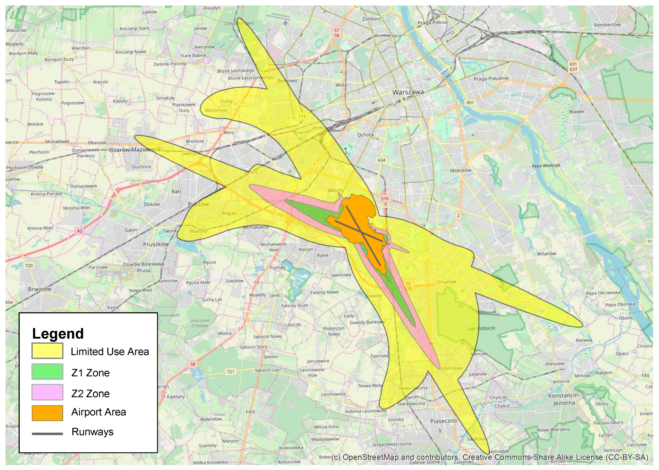
Prohibition to design the areas in the spatial development plans for the development of single and multi-family houses (Z1), residential and commercial buildings (Z1), buildings for short or long-term stays of children and young people (Z1, Z2), hospitals and social welfare homes (Z1, Z2);
-
Prohibition to changes to the function of existing ones—prohibition to changes to the function of existing ones: residential buildings (Z1), buildings for short or long-term stays of children and young people (Z1, Z2), hospitals and social welfare homes (Z1, Z2);
-
An obligation to apply anti-noise protection in newly designed and existing residential buildings (in the entire LUA area);
-
The necessity to endure noise exceeding acceptable standards (in the whole LUA area).
Residents of a limited use area (LUA) may claim compensation for restrictions on the use of their property or even demand the purchase of all or part of the real estate. Thus, the main goal of our research is to determine the differences in prices between real estate located within the LUA and outside this zone.
The study used 288 transactions of sales of single-family houses (2013–2017), derived from the register of real estate price and value kept by the Municipal Office in Warsaw and the relevant Poviat Administrator’s Office. More specifically, the prices of 1 m2 of single-family houses (typical, two-storey detached, semi-detached, and terraced buildings) from the resale market, located within the Warsaw Chopin Airport’s impact zone, were adopted for the analysis. During the period under analysis, 78 house sale transactions took place within the limited use area (LUA), which accounts for 27% of the total number of transactions, while 211 transactions were carried out outside this zone (LUA_OUT). Basic descriptive statistics are presented in Table 1.
Figure 2 shows the scatter plot of real estate unit prices over time for both tested groups of single-family house prices. Interpenetrating distributions of residential real estate prices within the LUA and outside the LUA are noticeable. However, within the entire group, single-family houses located outside the LUA tend to obtain higher prices than those located within the LUA.
For the purposes of the construction of the classic multiple regression model, the spatial autoregressive model (SAR), and the geographically weighted regression (GWR) model, the logarithm of the price of 1 m2 of a single-family house was adopted as the response variable instead of the real estate price. The adoption of the algorithm was dictated by both the relatively large differences in prices and the distribution characterised by strong negative skew. Each of the adopted 288 real estate sale transactions is also described with a number of attributes that are explanatory variables in the applied statistical models. The source of the description of data for explanatory variables was cadastral data acquired from the Warsaw Municipal Office and Poviat Administration Offices, Open Street and an own field visit. As a result, a set of variables was defined, along with their characteristics presented in Table 2.

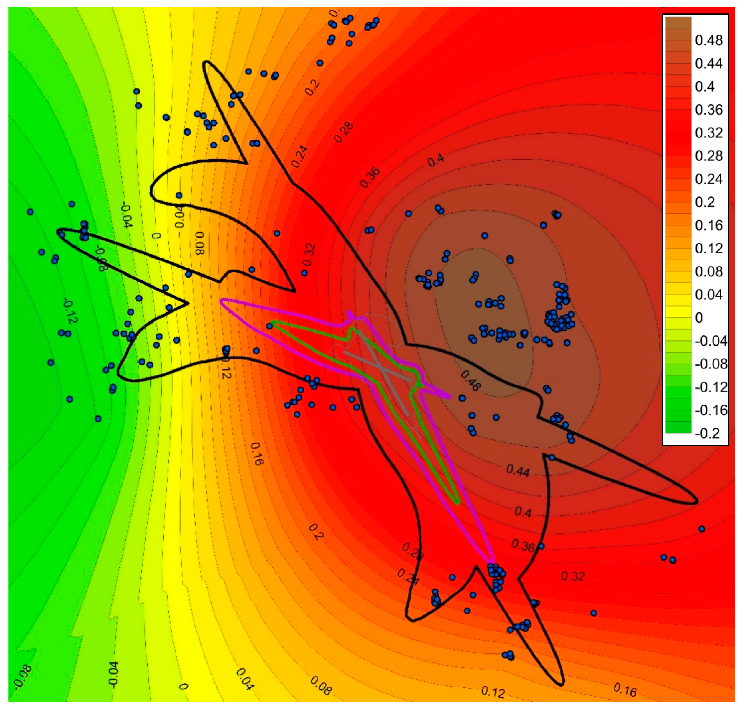
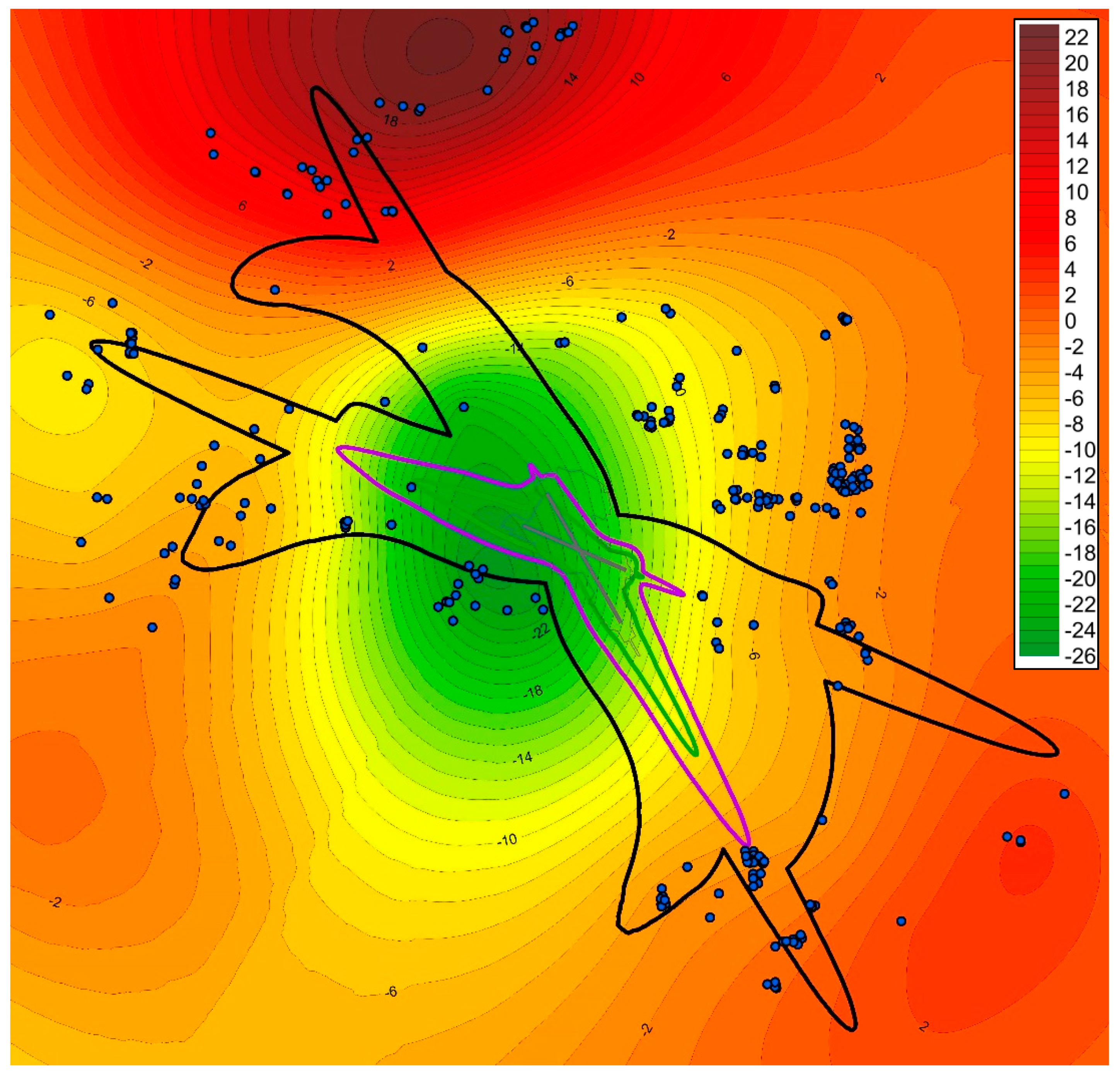
4. Results and Discussion

In order to identify the magnitude of impact of the Warsaw Chopin Airport’s effects on the spatial development of prices of real estate with single-family houses, three statistical models were developed, namely:
-
A multiple regression model;
-
A spatial autoregressive model (SAR);
-
A geographically weighted regression model (GWR).
For the purposes of the construction of the multiple regression model, the following were adopted as explanatory variables: the state of development (SZ), additional buildings on the plot (DB), building type (FZ), floor area of a single-family house (PU), plot area (PD), distance from the airstrip at the airport (OP), and the location within and outside of the Chopin Airport’s LUA. Model estimation results are presented in Table 3.
All variables adopted for the analysis were characterised by statistically significant, estimated parameters (p < 0.05). At the same time, the parameter standing by the LUA variable (location within the limited use area) proved to be the most statistically significant. The value of this parameter, at the variable of the impact of location over the limited use area, amounts to −31.11 (i.e., e−0.3727−1). Based on this parameter, it can be concluded that the average price of real estate located within the LUA is lower by 31.11% than real estate located outside this area. However, the coefficient of fitting of the multiple regression model to empirical data, measured using the determination coefficient (R2 = 0.26), is rather low, and therefore the obtained result is uncertain.
During the analyzes, it was found that there is a significant spatial autocorrelation of transaction prices (logarithms from prices). Moran I’s spatial autocorrelation coefficient was 0.3425 (Figure 3). On this basis, it can be concluded that the use of spatial autoregressive models is justified.
For the purposes of the construction of the SAR model, the following were adopted as explanatory variables: the state of repair and functional condition (STU), the state of development (SZ), additional buildings on the plot (DB), building type (FZ), floor area of a single-family house (PU), plot area (PD), and the location within and outside of the Chopin Airport’s limited use area (LUA). Model estimation results are presented in Table 4.
For most of the variables left in the spatial autoregressive model, the estimated parameters are statistically significant. Estimation of the parameter with the LUA variable, i.e., the impact of location within the limited use area and outside it is statistically significant (p < 0.01). It can therefore be concluded that unit prices of single-family houses located within the LUA are lower by about 14% (i.e., e−0.152−1) than the prices of real estate outside the LUA. Figure 4 shows a visualisation of the spatial component of the spatial delay model resulting from spatial autocorrelation of transaction prices, expressed as signal = λWy. The logarithm of this impact ranged from −0.159 to +0.182, hence the relative impact ranges from −15% to 20%.
For the purposes of the GWR model construction with reference to the relationship of the logarithm of the price of 1 m2 of a single-family house to a single explanatory variable that defines the location both within and outside the limited use area (LUA), the βOOU coefficient was determined. The spatial diversity of the βOOU coefficient value in the log-linear GWR model indicates that an adverse impact of the LUA variable may be observed mainly in the western part of the area under analysis (Figure 5) and may reach the value of −13% (i.e., e−0.143−1). In the eastern part, however, the impact is negative and amounts to as much as 60% (i.e., e0.489−1). At the same time, the value of statistics t indicates that, within this area, this is a statistically significant variable.
The spatial diversity of the rate of changes in single-family house prices, estimated based on the GWR model with a single explanatory variable (Data), indicates a downward trend in the unit prices in the vicinity of the airport (up to 25% per annum), while at a greater distance, the trend in the price change is positive (Figure 6). This enables the suggestion of a hypothesis that the proximity of an airport has an adverse effect on the rate of increase in prices. However, the spatial distribution of the price change coefficient does not coincide with the limited use area, yet the centre of the lowest values is located in the central part of the airport in Warsaw.

5. Conclusions

Proximity to an airport involves nuisance resulting primarily from the exceeding of environmental protection standards related to noise. Not only does the nuisance result from the actual exposure to an excessive noise level, but also from legal restrictions associated with the introduction of the LUA. The conducted study indicates that the real estate market reflects this nuisance in the form of lower prices of real estate located within the limited use area in the vicinity of the airport. Both the classic multiple regression model and the spatial autoregressive model indicate that the variable indicating the location of real estate within the LUA is statistically significant, with the prices of real estate in the vicinity of the airport being lower by 14% to 30% than the prices of real estate located outside the limited use area. Moreover, the geographically weighted regression model indicates that the proximity to an airport adversely affects the rate of price changes due to the passage of time.
The results of the conducted study confirm that the real estate market significantly responds to the nuisance related to the effects of Warsaw Chopin Airport. This is an important premise for making decisions on the compensation related to a decrease in real estate value, and on funding the costs of an improvement of the acoustic value of buildings exposed to excessive noise.

Author Contributions

Conceptualization, Radosław Cellmer and Mirosław Bełej; Data curation, Jan Konowalczuk; Formal analysis, Radosław Cellmer and Mirosław Bełej; Investigation, Jan Konowalczuk; Methodology, Radosław Cellmer and Mirosław Bełej; Visualization, Radosław Cellmer and Mirosław Bełej The participation of the first two authors is equal in value.

Funding

This research received no external funding.

Acknowledgments

The authors express sincere gratitude to the Journal Editor and the anonymous reviewers who spent their valued time to provide constructive comments and assistance to improve the quality of this paper.

Conflicts of Interest

The authors declare no conflicts of interest.

Abbreviations

LUALimited use area
LUA_OUTLimited use area (outside)
GWRGeographically weighted regression
SARSpatial autoregressive model

References

  1. Cooper, R. Airports and economic development: An overview. Transp. Res. Rec. 1990, 125–133. [Google Scholar]
  2. Green, R.K. Airports and economic development. Real Estate Econ. 2007, 35, 91–112. [Google Scholar] [CrossRef]
  3. Button, K.; Doh, S.; Yuan, J. The role of small airports in economic development. J. Airpt. Manag. 2010, 4, 125–136. [Google Scholar]
  4. Warffemius, P.; Van der Hoorn, T.; Klaassen, H. The importance of agglomeration effects for distribution centres around Amsterdam Airport Schiphol. J. Airpt. Manag. 2010, 4, 265–279. [Google Scholar]
  5. Costa, V.; Almeida, C. Low-Cost Carriers Local Economy and Tourism Development at Four Portuguese Airports. A Model of Cost–Benefit Analysis. J. Spat. Organ. Dyn. 2015, 3, 245–261. [Google Scholar]
  6. Trojanek, R.; Tanaś, J.; Raslanas, S.; Banaitis, A. The impact of aircraft noise on housing prices in Poznan. Sustainability 2017, 9, 2088. [Google Scholar] [CrossRef]
  7. Batóg, J.; Foryś, I.; Gaca, R.; Głuszak, M.; Konowalczuk, J. Investigating the Impact of Airport Noise and Land Use Restrictions on House Prices: Evidence from Selected Regional Airports in Poland. Sustainability 2019, 11, 412. [Google Scholar] [CrossRef]
  8. Sedoarisoa, N.; Desponds, D.; Dalmas, L.; Lavandier, C. Housing prices and the proximity of the Paris–Charles-de-Gaulle (CDG) airport. L’Espace Géograph. 2017, 46, 61–78. [Google Scholar] [CrossRef]
  9. Kaufman, H.F.; Espey, M.; Englin, J.E. No plane, big gain? airport noise and residential property values in the Reno-Sparks area. Choices 1998, 13. [Google Scholar] [CrossRef]
  10. Espey, M.; Lopez, H. The impact of airport noise and proximity on residential property values. Growth Chang. 2000, 31, 408–419. [Google Scholar] [CrossRef]
  11. Mark, J.; Goldberg, M.A. Multiple regression analysis and mass assessment: A review of the issues. Apprais. J. 1998, 56, 89. [Google Scholar]
  12. Bowen, W.M.; Mikelbank, B.A.; Prestegaard, D.M. Theoretical and empirical considerations regarding space in hedonic housing price model applications. Growth Chang. 2001, 32, 466–490. [Google Scholar] [CrossRef]
  13. Bourassa, S.C.; Cantoni, E.; Hoesli, M. Predicting House Prices with Spatial Dependence: A Comparison of Alternative Methods. J. Real Estate Res. 2010, 32, 139–160. [Google Scholar]
  14. LeSage, J.P.; Pace, R.K. Introduction to Spatial Econometrics; CRC Press: Boca Raton, FL, USA, 2009. [Google Scholar]
  15. Anselin, L. Spatial Dependence and Spatial Structural Instability in Applied Regression Analysis. J. Reg. Sci. 2006, 30, 185–207. [Google Scholar] [CrossRef]
  16. Longford, N. Random Coefficient Models; Oxford University Press: Oxford, UK, 1995. [Google Scholar]
  17. Andersson, H.; Jonsson, L.; Ögren, M. Property prices and exposure to multiple noise sources: Hedonic Regression with road and railway noise. Environ. Resour. Econ. 2010, 45, 73–89. [Google Scholar] [CrossRef]
  18. Fotheringham, A.S.; Brunsdon, C.; Charlton, M. Geographically Weighted Regression: The Analysis of Spatially Varying Relationships; John Wiley & Sons: Hoboken, NJ, USA, 2002. [Google Scholar]
  19. Conway, D.; Li, Q.C.; Wolch, J.; Kahle, C.; Jerrett, M. A Spatial Autocorrelation Approach for Examining the Effects of Urban Greenspace on Residential Property Values. J. Real Estate Fin. Econ. 2010, 41, 150–169. [Google Scholar] [CrossRef]
  20. Arbia, G. Spatial Econometrics: Statistical Foundations and Applications to Regional Convergence; Springer: Berlin, Germany, 2006. [Google Scholar]
  21. Besner, C. A spatial autoregressive specification with a comparable sales weighting scheme. J. Real Estate Res. 2002, 24, 193–211. [Google Scholar]
  22. Charlton, M.; Fotheringam, S. Geographically Weighted Regression; White Paper; National University of Ireland Maynooth: Maynooth, Ireland, 2009. [Google Scholar]
  23. Brunsdon, C.; Fotheringham, A.S.; Charlton, M.E. Geographically weighted regression: A method for exploring spatial nonstationarity. Geogr. Anal. 1996, 28, 281–298. [Google Scholar] [CrossRef]
  24. Manganelli, B.; Pontrandolfi, P.; Azzato, A.; Murgante, B. Using geographically weighted regression for housing market segmentation. Int. J. Bus Intell. Data Min. 2014, 9, 161–177. [Google Scholar] [CrossRef]
  25. Yang, S.; Hu, S.; Li, W.; Zhang, C.; Torres, J.A. Spatiotemporal Effects of Main Impact Factors on Residential Land Price in Major Cities of China. Sustainability 2017, 9, 2050. [Google Scholar] [CrossRef]
  26. Lu, B.; Charlton, M.; Fotheringhama, A.S. Geographically weighted regression using a non-Euclidean distance metric with a study on London house price data. Proc. Environ. Sci. 2011, 7, 92–97. [Google Scholar] [CrossRef]
  27. Wu, H.; Jiao, H.; Yu, Y.; Li, Z.; Peng, Z.; Liu, L.; Zeng, Z. Influence Factors and Regression Model of Urban Housing Prices Based on Internet Open Access Data. Sustainability 2018, 10, 1676. [Google Scholar] [CrossRef]
  28. Dziauddin, M.F.; Powe, N.; Alvanides, S. Estimating the Effects of Light Rail Transit (LRT) System on Residential Property Values Using Geographically Weighted Regression (GWR). Appl. Spat. Anal. Policy 2015, 8, 1–25. [Google Scholar] [CrossRef]
  29. Wu, B.; Li, R.; Huang, B. A geographically and temporally weighted autoregressive model with application to housing prices. Int. J. Geogr. Inf. Sci. 2014, 28, 1186–1204. [Google Scholar] [CrossRef]
  30. McCord, M.; Davis, P.T.; Haran, M.; McGreal, S.; McIlhatton, D. Spatial variation as a determinant of house price: Incorporating a geographically weighted regression approach within the Belfast housing market. J. Financ. Manag. Prop. Constr. 2012, 17, 49–72. [Google Scholar] [CrossRef]
  31. Cellmer, R.; Bełej, M.; Źrobek, S.; Kovač, M.Š. Urban land value maps–a methodological approach. Geod. Vestn. 2014, 58, 535–551. [Google Scholar] [CrossRef]
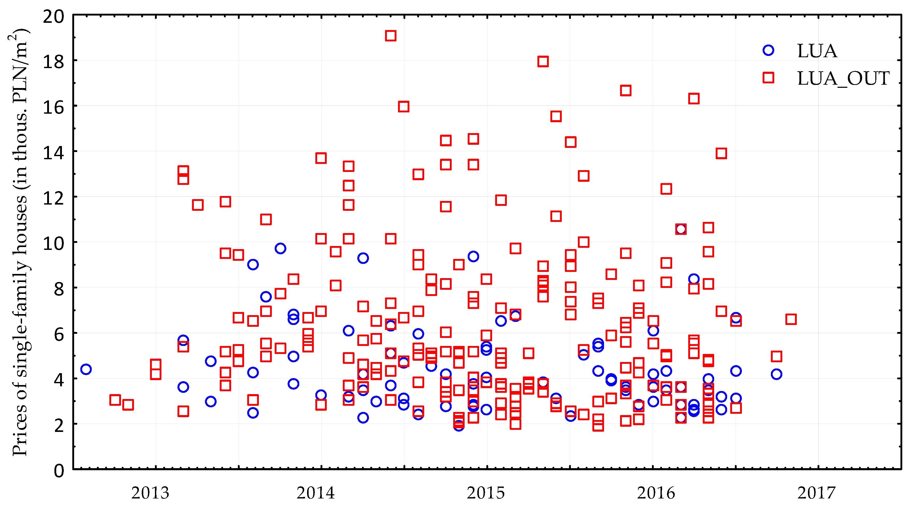
Figure 1. Localization of Warsaw Chopin Airport and limited use area (LUA).
Ijgi 08 00471 g001
Figure 2. The scatter plot of 289 sale prices of single-family houses in the years 2013–2017.
Ijgi 08 00471 g002
Figure 3. Moran’s scatterplot. Standarized logarithm of prices vs. spatially lagged standarized logarithm of prices. Moran I stat. st. dev.: 18.263, p-value < 2.2 × 10⁻¹⁶, Moran I statistic: 0.3425, Expectation: −0.0035, Variance: 0.00035.
Ijgi 08 00471 g003
Figure 4. Visualisation of the autoregressive component in the spatial lag model.
Ijgi 08 00471 g004
Figure 5. βLUA coefficient value in the GWR model. βLUA coefficient can be interpreted as a percentage (decimal) effect on prices.
Ijgi 08 00471 g005
Figure 6. Average annual price change (expressed in %) calculated based on the βDate coefficient in the GWR model.
Ijgi 08 00471 g006
Table 1. Basic descriptive statistics for 288 housing prices.
StatisticsLUA (PLN/m2)LUA_OUT (PLN/m2)
Average4356.956438.54
Median3917.195340.91
Standard deviation1820.183589.27
Number of observations78210
Min1704.551923.08
Max9717.9519107.39
25% quantile30003611.11
75% quantile5225.538252.43
Table 2. Description of variables.
SymbolDescription
Ln_Pricelogarithm of unit housing price in PLN/m2.
STUthe state of repair and functional condition of a single-family house: to be demolished −1, (minus) intermediate −2, intermediate −3, (plus) intermediate −4, favourable −5.
SZthe state of development: poor −1, average −2, favourable −3.
DBadditional buildings: none −1, present −2.
OTsurroundings: deteriorated −1, average −2, favourable −3.
LUAWarsaw Chopin Airport’s LUA: location outside the LUA −0, location within the LUA −1.
OPdistance from the airstrip, in metres
FZbuilding type: rowhouse −1, semi-detached house, end-of-terrace house −2, detached building −3.
PDplot area; quantitative continuous cadastral area.
PUfloor space of a single-family house: quantitative continuous area calculated as the product of the gross covered area and the number of storeys but with account taken of the irregularity of solids.
LSlocation quality; 4 − grade assessment.
Table 3. Multiple regression model.
VariableEstimateStandard Errort valuePr(>|t|)
(Intercept)9.17410.172953.061< 2 × 10⁻¹⁶***
SZ−0.21140.04934.2902.12 × 10−5***
DB−0.20790.0511−4.0676.18 × 10−5***
FZ−0.13240.0496−2.6710.00801*
PU−0.00130.0004−3.4810.00058***
PD0.00040.00012.9110.00389**
OP−0.05130.0101−5.0836.79 × 10−7***
LUA0.37270.06176.0424.82 × 10−9***
Significance codes: 0 ‘***’ 0.001 ‘**’ 0.01 ‘*’ 0.05 ‘.’ 0.1 ‘’ 1, Residual standard error: 0.4559 on 281 degrees of freedom, Multiple R-squared: 0.2643, Adjusted R-squared: 0.246, F-statistic: 14.42 on 8 and 281 DF, p-value: < 2.2 × 10⁻¹⁶.
Table 4. Spatial autoregressive model.
VariableEstimateStandard Errort valuePr(>|t|)
(Intercept)0.28740.16861.70450.0882.
STU0.02810.03430.82070.4118
SZ0.15340.04433.46210.0005***
DB−0.13520.0390−3.46460.0005***
FZ−0.07460.0375−1.98790.0468*
PU−0.00162.92 × 10−4−5.39326.92 × 10−8***
PD3.00 × 10−49.43 × 10−53.17770.0015**
LUA0.15290.04693.26100.0011**
Significance codes: 0 ‘***’ 0.001 ‘**’ 0.01 ‘*’ 0.05 ‘.’ 0.1 ‘’ 1, Rho: 0.97824, LR test value: 149.95, p-value: < 2.22 × 10⁻¹⁶, Asymptotic standard error: 0.014084, z-value: 69.46, p-value: < 2.22 × 10⁻¹⁶, Wald statistic: 4824.7, p-value: < 2.22 × 10⁻¹⁶, Log likelihood: −116.3404 for lag model, AIC: 252.68, (AIC for lm: 400.3), ML residual variance (sigma squared): 0.12024, (sigma: 0.34675), LM test for residual autocorrelation, test value: 25.698, p-value: 3.992 × 10⁻⁷.

