Spatial Context-Based Local Toponym Extraction and Chinese Textual Address Segmentation from Urban POI Data


Abstract
:1. Introduction
2. Background and Related Work
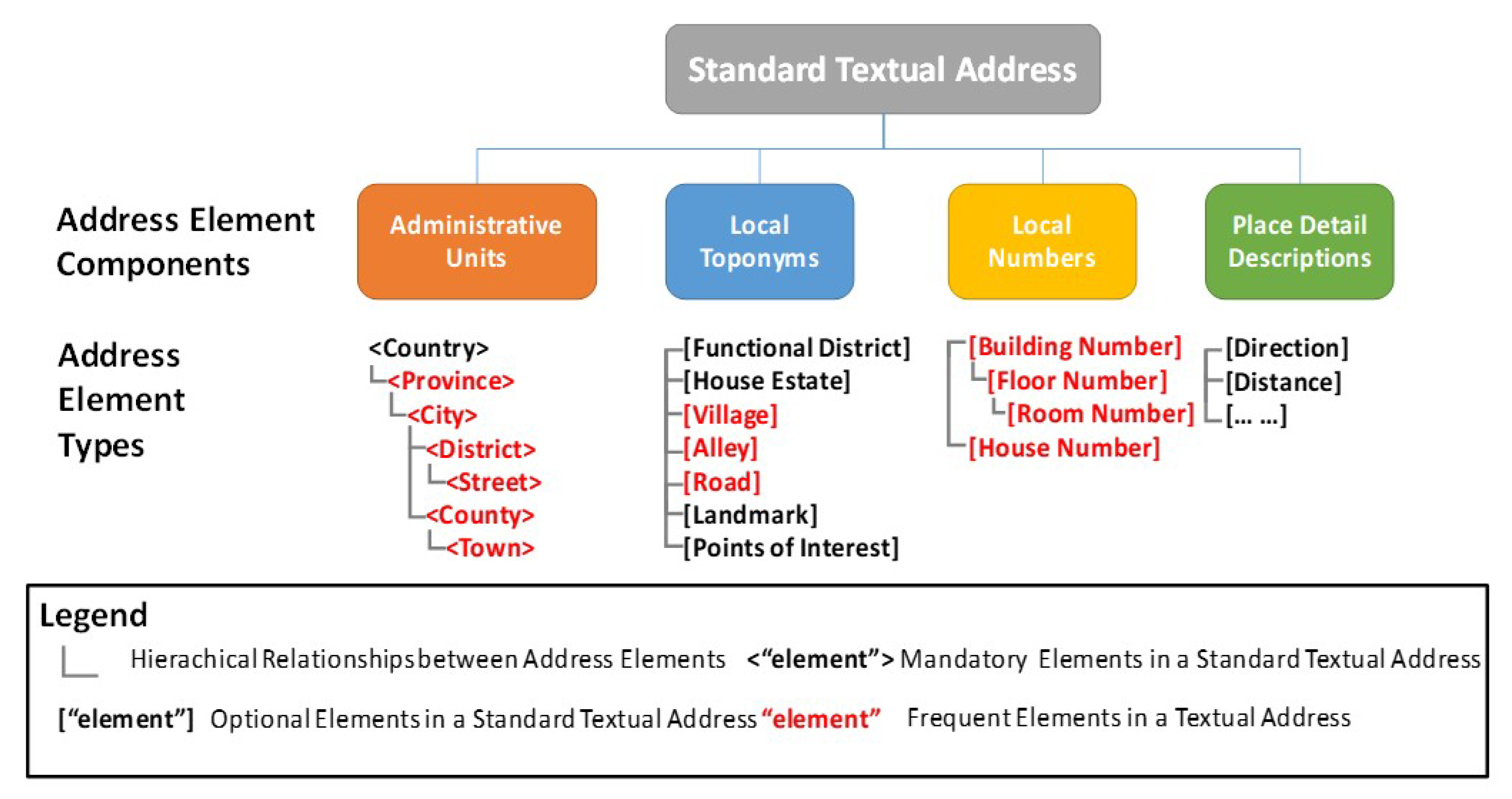
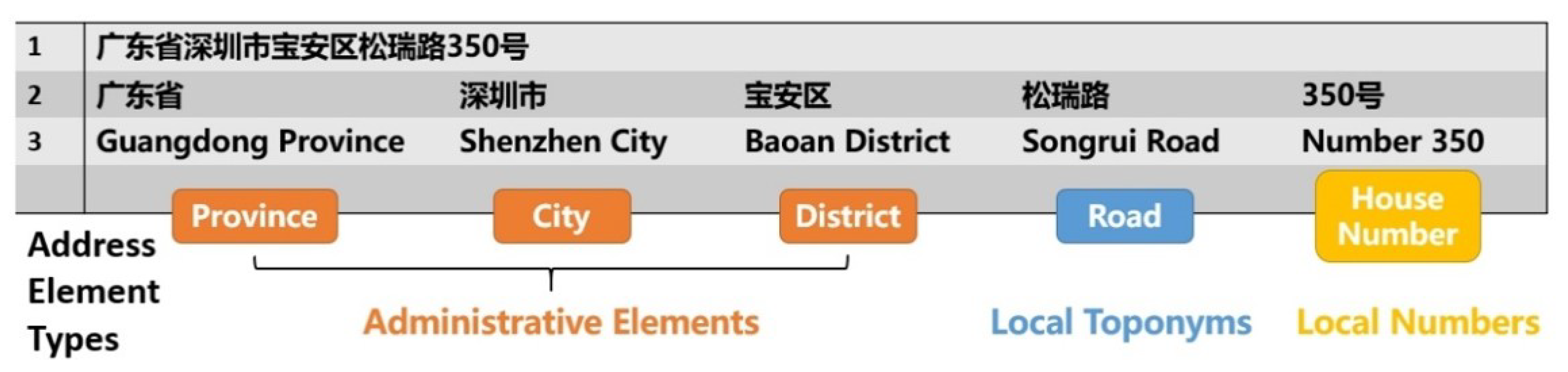
2.1. Background Knowledge
2.2. Related Work
3. Method
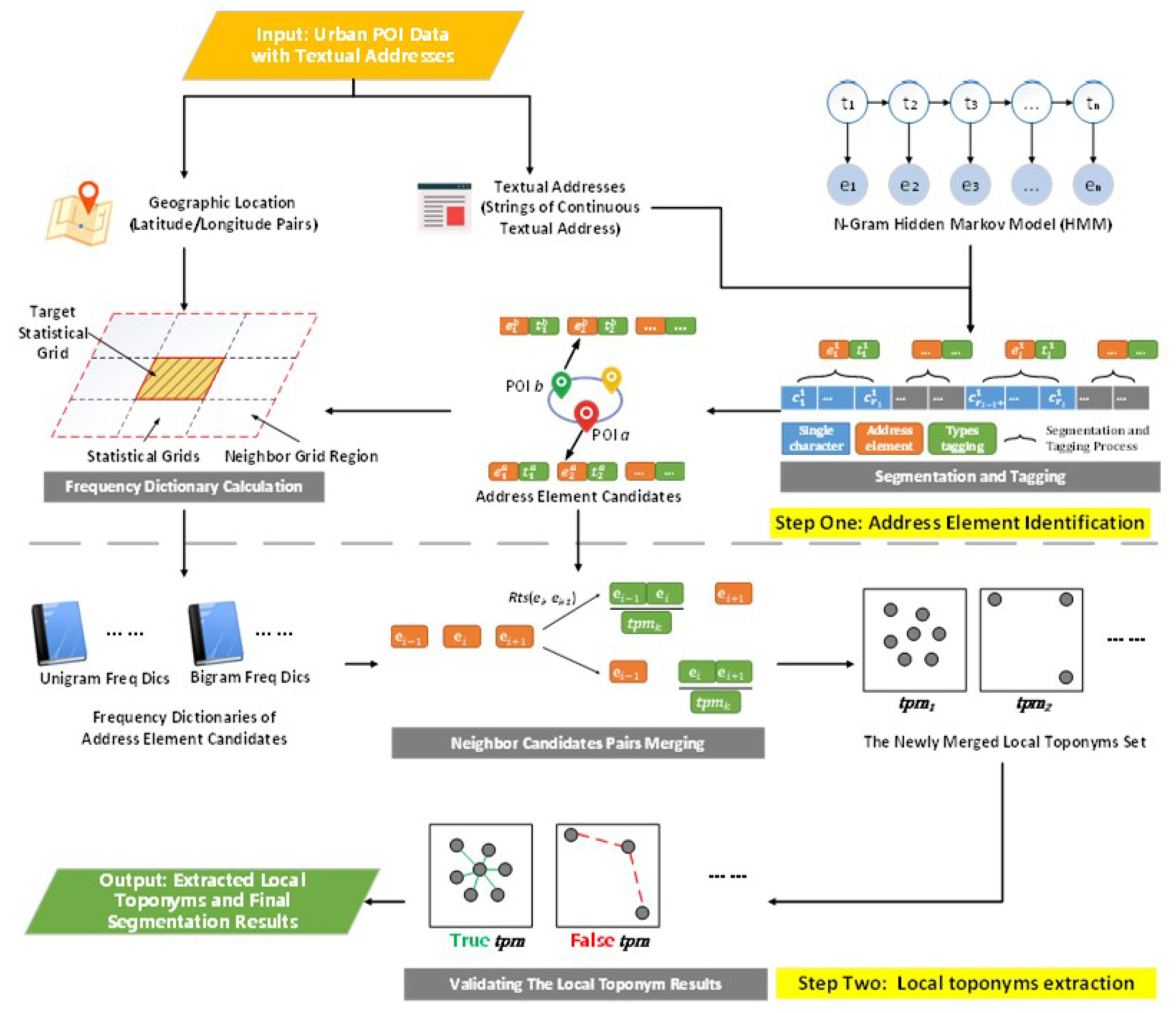
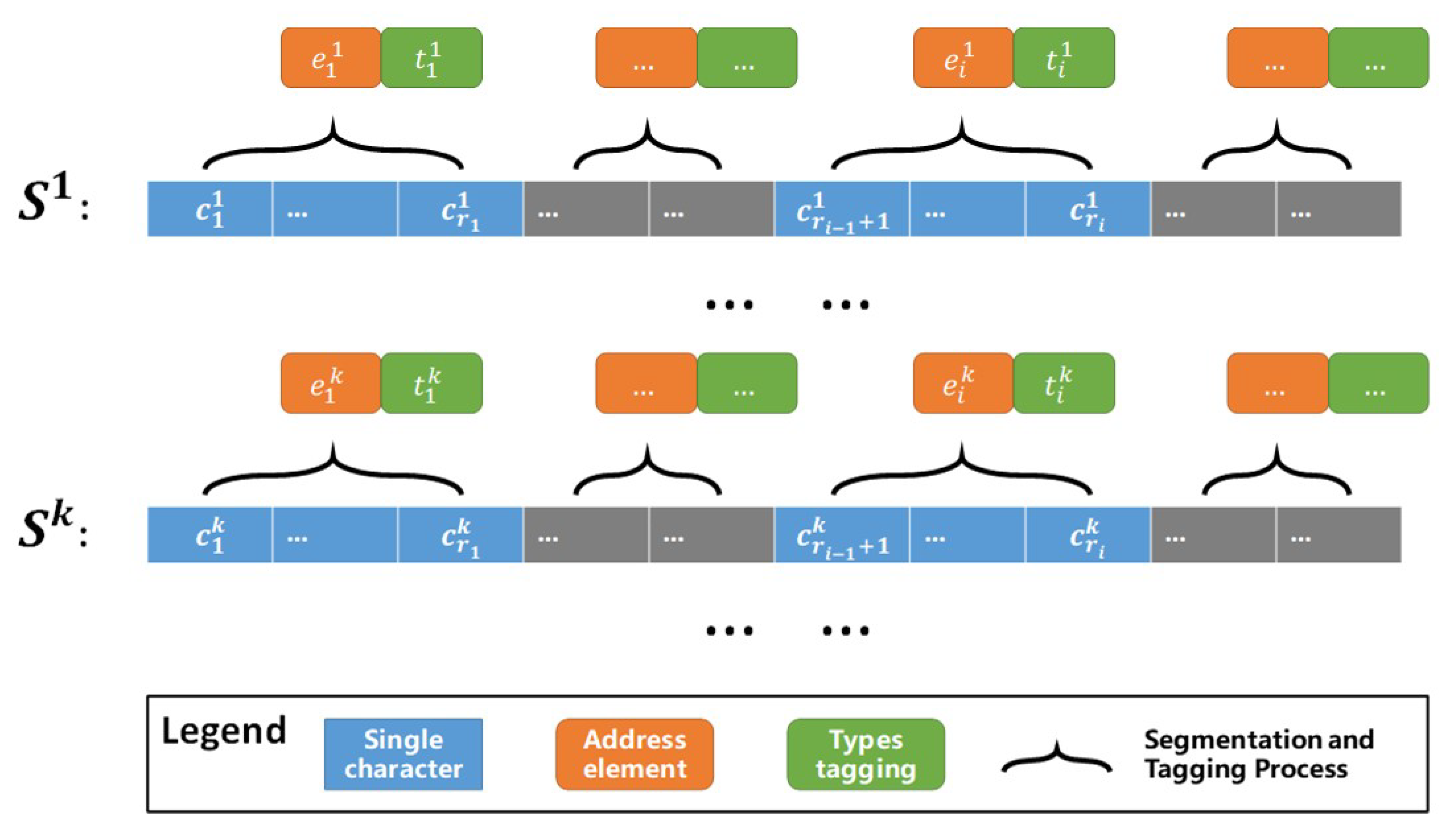
3.1. Input: Urban POI Data with Textual Addresses
3.2. Step One: Address Element Identification
3.3. Step Two: Local Toponyms Extraction
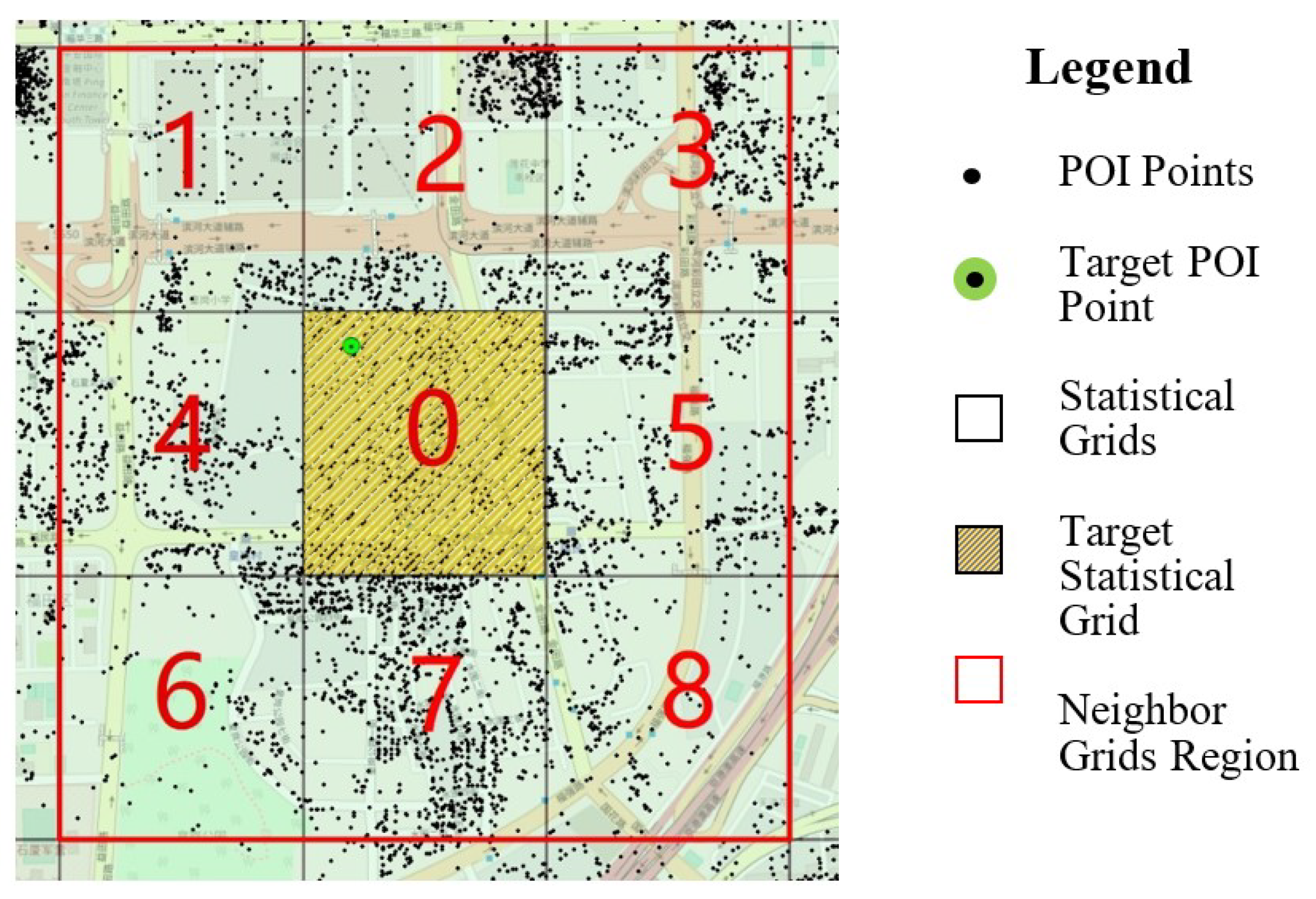
3.3.1. Exploration of Local Toponym Spatial Distribution Patterns
| Algorithm 1:Frequency dictionary calculation | |
| Input: | |
| 1. The rough segmentation results of the target POI’s textual address is sT (e1, e2, …, ei), where ei is the address element candidate segmented from the textual address of the target POI; | |
| 2. The rough segmentation results of other POIs within the neighbor grids region is S^(s1, s2, …, sn). | |
| Output: The unigram and bigram frequency dictionaries, D-1 and D-2. | |
| def Uni-gram frequency dictionary calculation: | |
| Initialization: | |
| 1: | Initialize uni-gram frequency dictionary D-1[str, count], in which ‘str’ is the uni-gram keyword and ‘count’ is the frequency of ‘str’ |
| Iteration: | |
| 2: | for each address element candidate, ei sT do |
| 3: | D-1.append(ei, 1) |
| 4 | end for |
| 5: | for each rough segmentation results, sj S^ do |
| 6: | for each address element candidate, ek sj do |
| 7: | if ek is the key of D-1 |
| 8 | D-1[ek] += 1 |
| 9 | end if |
| 10: | end for |
| 11: | end for |
| 12: | returnD-1 |
| def Bigram frequency dictionary calculation: | |
| Initialization: | |
| 1: | Initialize bi-gram frequency dictionary D-2[str, count], in which ‘str’ is the bi-gram keyword and ‘count’ is the frequency of ‘str’ |
| Iteration: | |
| 2: | for each address element candidate, ei sT do |
| 3: | D-2.append(ei + ei+1, 1) |
| 4 | end for |
| 5: | for each rough segmentation results, sj S^ do |
| 6: | for each address element candidate, ek sj do |
| 7: | if (ek + ek+1) is_the_key of D-2 |
| 8 | D-2[ek + ek+1] += 1 |
| 9 | end if |
| 10: | end for |
| 11: | end for |
| 12: | returnD-2 |
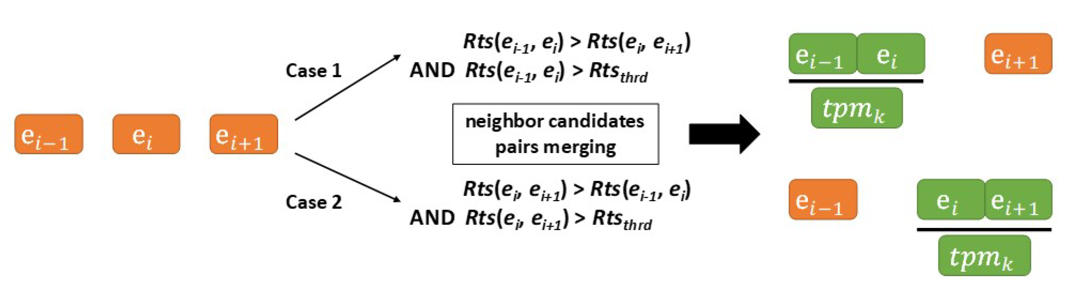
3.3.2. Merging Neighbor Candidate Pairs
| Algorithm 2:Neighbor candidates pairs merging | |
| Input: | |
| 1. The rough segmentation results of the target POI, sT (e1, e2, …, ei), where ei is the address element candidate segmented from the textual address of the target POI; | |
| 2. The unigram and bigram frequency dictionaries, D-1 and D-2. | |
| Output: The newly merged local toponyms set, Tpm (tpm1, tpm2, …, tpmk). | |
| def Merging neighboring candidate pairs: | |
| Initialization: | |
| 1. | Initialize The newly merged local toponyms set Tpm [] |
| Iteration: | |
| 2. | for each address element candidate, ei sT do |
| 3. | Calculate Rts(ei−1, ei) based on Equation (5) |
| Calculate Rts(ei, ei+1) based on Equation (5) | |
| 4. | if Rts(ei−1, ei) > Rts(ei, ei+1) && Rts(ei−1, ei) > Rtsthrd |
| Merge ei−1 and ei into tpmk | |
| Tpm.append (tpmk) | |
| 5. | else If Rts(ei, ei+1) > Rts(ei−1, ei) && Rts(ei, ei+1) > Rtsthrd |
| Merge ei+1 and ei+1 into tpmk | |
| Tpm.append (tpmk) | |
| 6. | end if |
| 7. | end for |
| 8. | doAlgorithm 1 based on new Tpm [] |
| 9: | repeat steps 2–8 until no more updates to tpm occur |
| 10: | returnTpm [] |
3.3.3. Validating the Local Toponym Results
| Algorithm 3: Local toponym clustering with SSI | |
| Input: 1. The newly extracted local toponym, tpmk; 2. The original urban POIs dataset (UPD) with textual addresses. | |
| Output: The entropy value E-tpmk, which measures the geospatial clustering degree for tpmk. | |
| def Local toponym clustering: | |
| Initialization: | |
| 1: | Initialize a set of POI points whose textual address contains tpmk |
| 2: | Initialize a set of distances R = {rm | m = 6, 7, 8, …, M}, in which rm = am, a = 2 meters |
| SQL Query: | |
| 3: | Select POIs from UPD |
| where textual addresses of POIs | |
| contains tpmk | |
| 4: | S-tpmk.append(POIs) |
| Iteration: | |
| 5: | for each distance threshold rkR do |
| 6: | define a set of connected point sets Gm [ |
| 7: | for each pairwise points Pti, Ptj S-tpmk do |
| 8: | Calculate the pairwise distances dij between |
| Pti and Ptj | |
| 9: | if dij < rm |
| 10: | if Pti in |
| 11: | .append(Ptj) |
| 12: | else if Ptj in |
| 13: | .append(Pti) |
| 14: | else |
| 15: | initialize a new |
| 16: | .append(Pti) |
| 17: | .append(Ptj) |
| 18: | end if |
| 19: | end for |
| 20: | Calculate Em based on Equation (6) |
| 21: | end for |
| 22: | Calculate E-tpmk based on Equation (7) |
| 23: | returnE-tpmk |
3.4. Output: Extracted Local Toponyms and Final Segmentation Results
4. Experiments
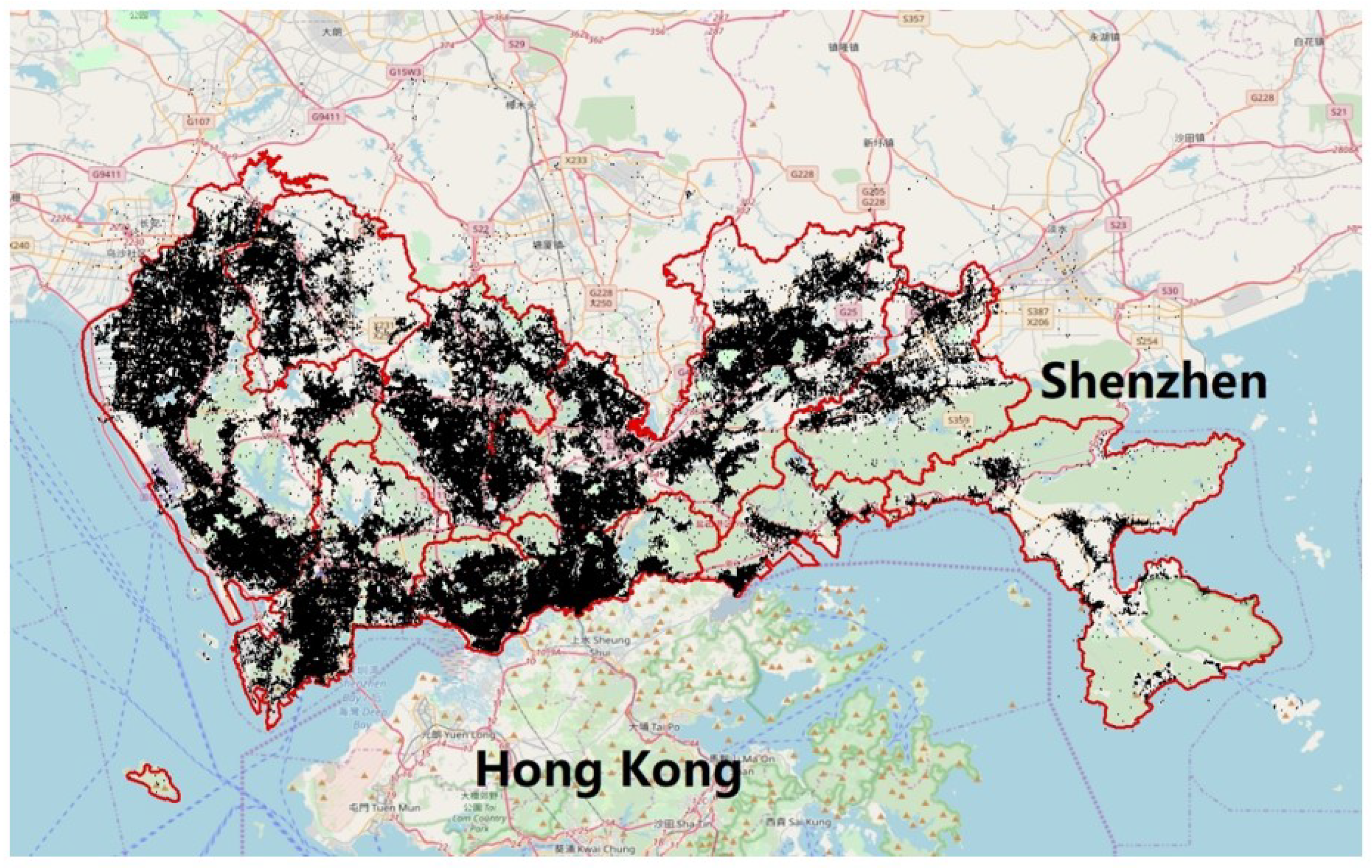
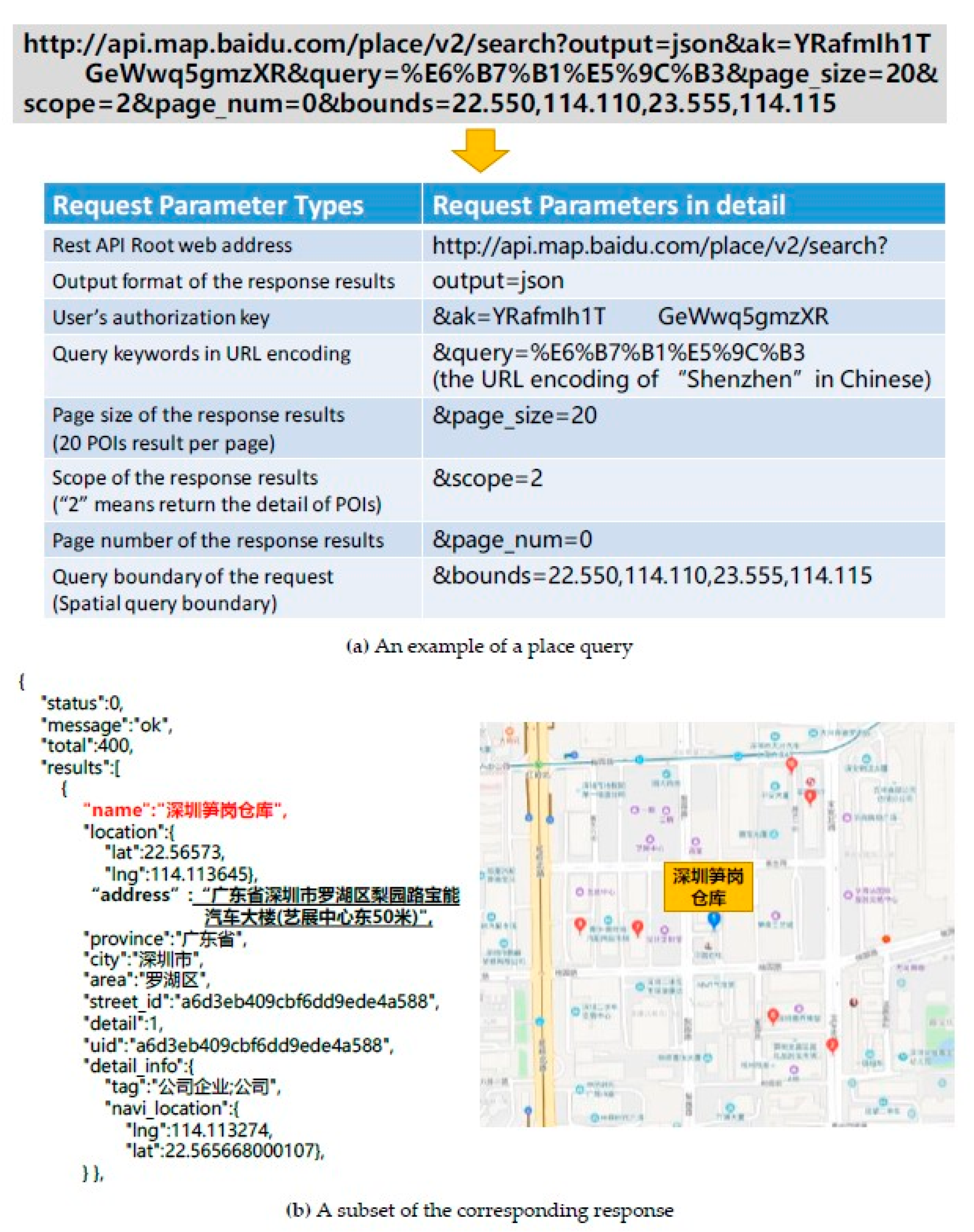
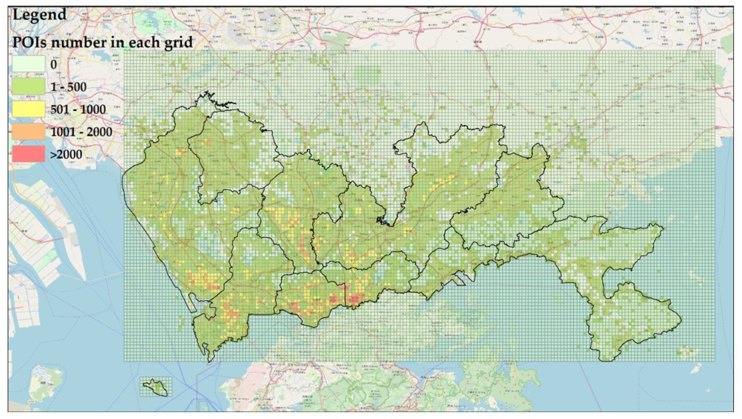
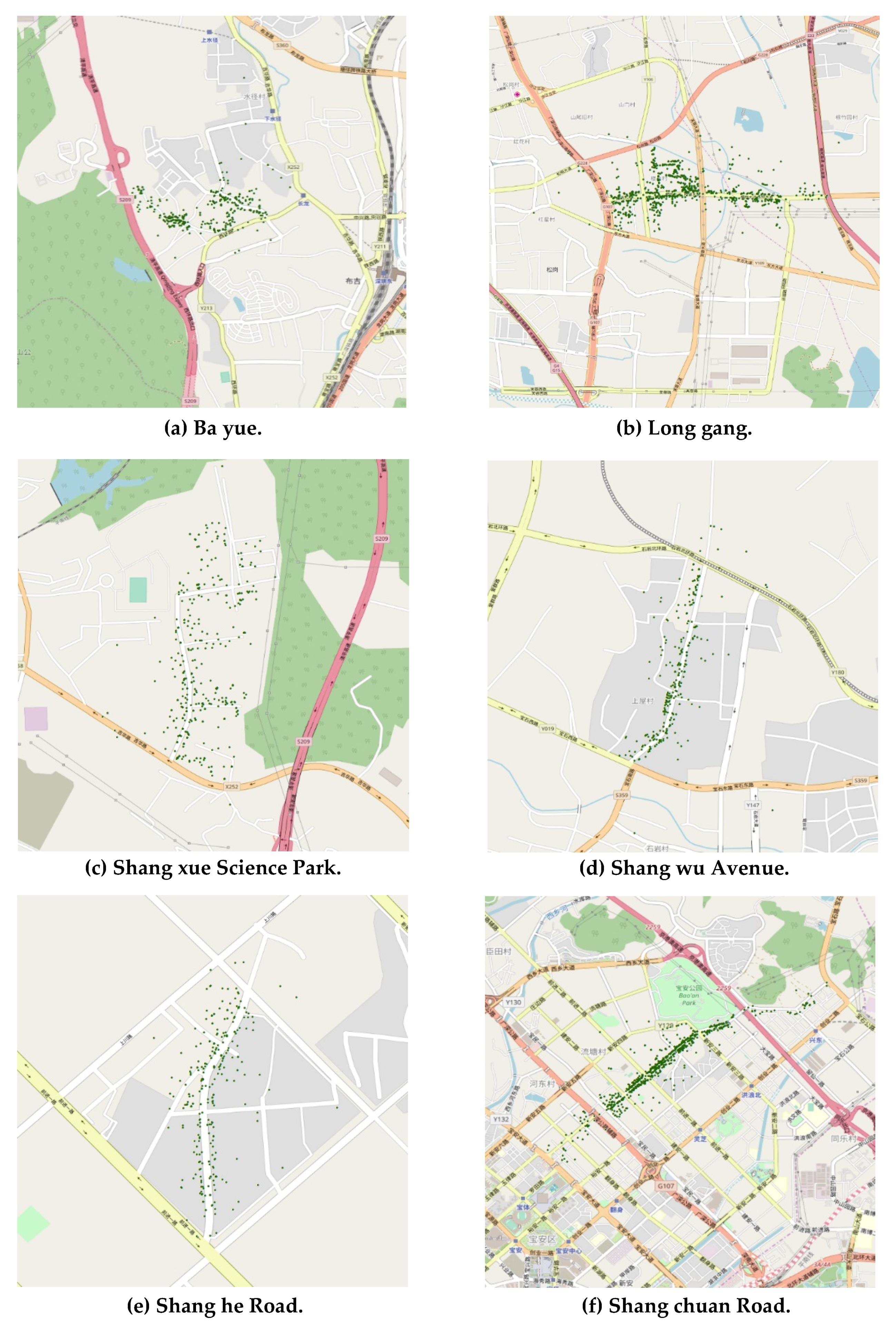
4.1. Dataset
4.2. Experimental Designs
4.3. Performance Evaluation
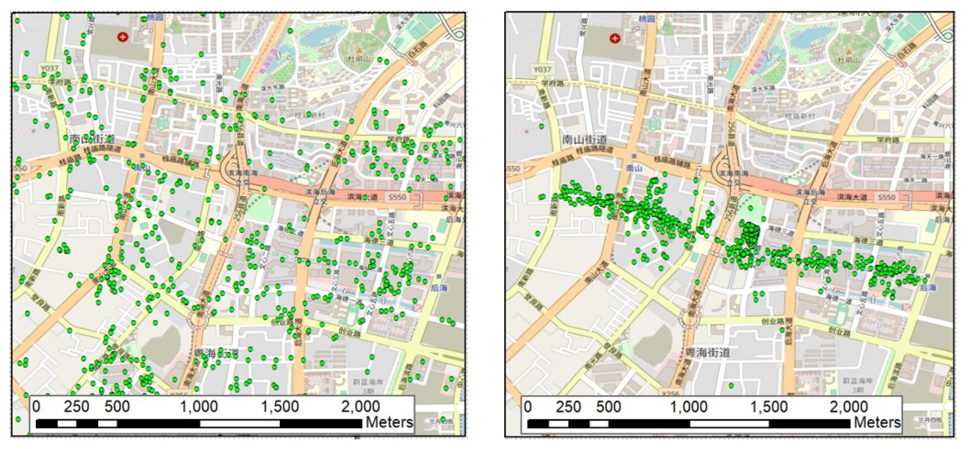
4.3.1. Ground-Truth Dataset Preparation
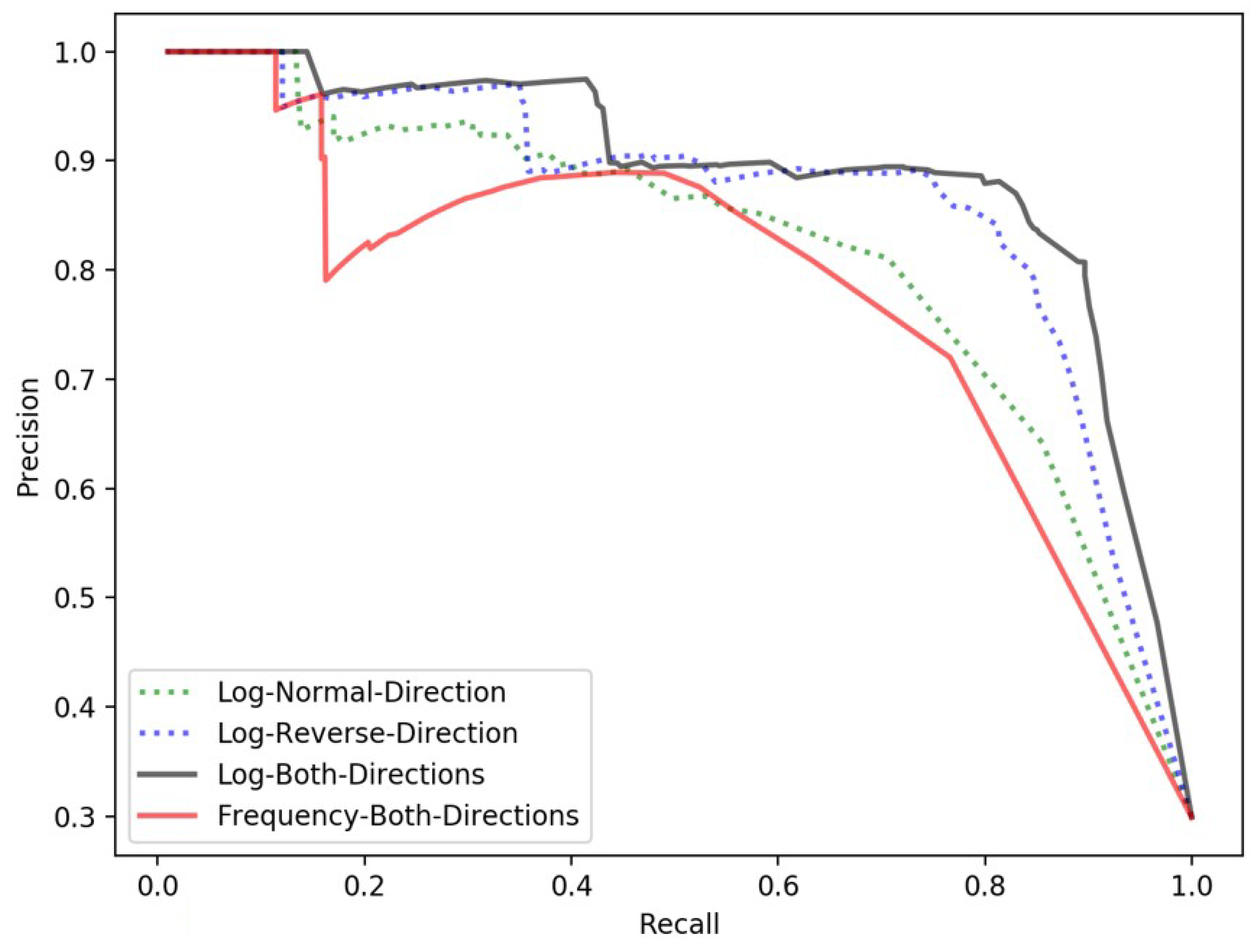
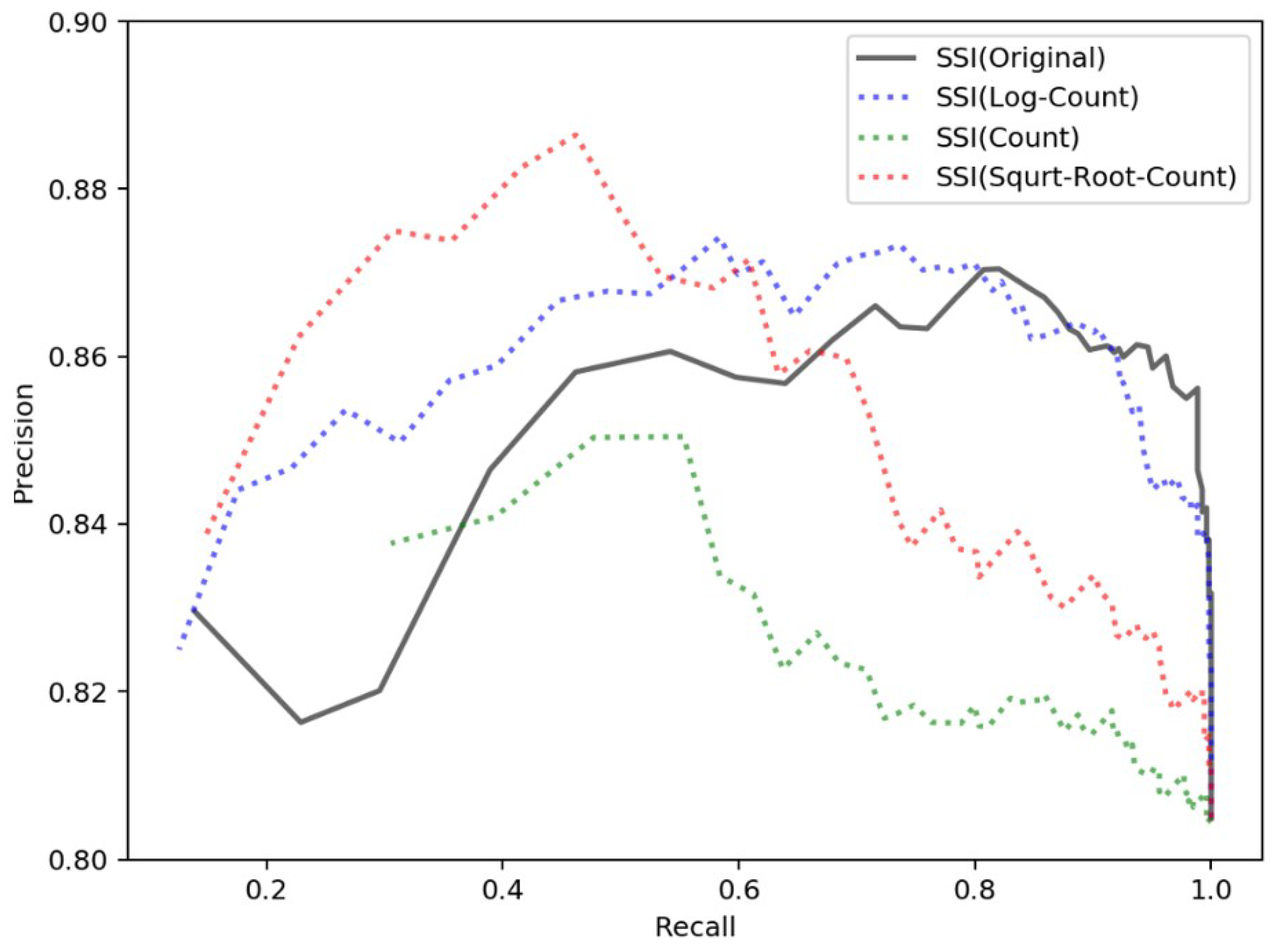
4.3.2. Threshold Determination for Extracting Local Toponyms
4.3.3. Performance Evaluation of the Two-Step Framework
- (a)
- jieba Word Segmenter (https://github.com/fxsjy/jieba);
- (b)
- HanLP Word Segmenter (https://github.com/hankcs/HanLP);
- (c)
- Stanford Word Segmenter (https://nlp.stanford.edu/software/segmenter.html).
5. Conclusions and Future Work
Author Contributions
Funding
Acknowledgments
Conflicts of Interest
References
- Roongpiboonsopit, D.; Karimi, H.A. Comparative evaluation and analysis of online geocoding services. Int. J. Geogr. Inf. Sci. 2010, 24, 1081–1100. [Google Scholar] [CrossRef]
- Hill, L.L. Georeferencing: The Geographic Associations of Information; MIT Press: Cambridge, MA, USA; London, UK, 2009. [Google Scholar]
- Zhu, R.; Hu, Y.; Janowicz, K.; McKenzie, G. Spatial signatures for geographic feature types: Examining gazetteer ontologies using spatial statistics. Trans. GIS 2016, 20, 333–355. [Google Scholar] [CrossRef]
- Goldberg, D.W. Advances in Geocoding Research and Practice. Trans. GIS 2011, 15, 727–733. [Google Scholar] [CrossRef]
- Li, L.; Wang, W.; He, B.; Zhang, Y. A hybrid method for Chinese address segmentation. Int. J. Geogr. Inf. Sci. 2017, 32, 30–48. [Google Scholar] [CrossRef]
- Oshikiri, T. Segmentation-Free Word Embedding for Unsegmented Languages. In Proceedings of the 2017 Conference on Empirical Methods in Natural Language Processing, Copenhagen, Denmark, 7–11 September 2017. [Google Scholar]
- Chowdhury, G.G. Natural language processing. Annu. Rev. Inf. Sci. Technol. 2003, 37, 51–89. [Google Scholar] [CrossRef] [Green Version]
- Hu, Y.; Mao, H.; McKenzie, G. A natural language processing and geospatial clustering framework for harvesting local place names from geotagged housing advertisements. Int. J. Geogr. Inf. Sci. 2018, 33, 714–738. [Google Scholar] [CrossRef]
- Kuo, C.-L.; Chan, T.-C.; Fan, I.-C.; Zipf, A. Efficient Method for POI/ROI Discovery Using Flickr Geotagged Photos. ISPRS Int. J. Geo-Inf. 2018, 7, 121. [Google Scholar] [CrossRef] [Green Version]
- GB/T 23705-2009: The Rules of Coding for Address in the Common Platform for Geospatial Information Service of Digital City; Standards Press of China: Beijing, China, 2009.
- W3C. Points of Interest. 2010. Available online: https://www.w3.org/2010/POI/wiki/Main_Page (accessed on 19 November 2019).
- Zhang, M.; Yu, N.; Fu, G. A Simple and Effective Neural Model for Joint Word Segmentation and POS Tagging. IEEE/ACM Trans. Audio Speech Lang. Process. 2018, 26, 1528–1538. [Google Scholar] [CrossRef]
- Kamper, H.; Jansen, A.; Goldwater, S. Unsupervised Word Segmentation and Lexicon Discovery Using Acoustic Word Embeddings. IEEE/ACM Trans. Audio Speech Lang. Process. 2016, 24, 669–679. [Google Scholar] [CrossRef]
- Eler, D.M.; Grosa, D.F.P.; Pola, I.; Garcia, R.; Correia, R.C.M.; Teixeira, J. Analysis of Document Pre-Processing Effects in Text and Opinion Mining. Information 2018, 9, 100. [Google Scholar] [CrossRef] [Green Version]
- Magistry, P.; Sagot, B. Unsupervized word segmentation: The case for Mandarin Chinese. In Proceedings of the 50th Annual Meeting of the Association for Computational Linguistics: Short Papers; Association for Computational Linguistics: Stroudsburg, PA, USA, 2012. [Google Scholar]
- Kang, M.; Du, Q.; Wang, M. A New Method of Chinese Address Extraction Based on Address Tree Model. Acta Geod. Cartogr. Sin. 2015, 44, 99–107. [Google Scholar]
- Tian, Q.; Ren, F.; Hu, T.; Liu, J.; Li, R.; Du, Q. Using an Optimized Chinese Address Matching Method to Develop a Geocoding Service: A Case Study of Shenzhen, China. ISPRS Int. J. Geo-Inf. 2016, 5, 65. [Google Scholar] [CrossRef] [Green Version]
- Zhou, H.; Du, Z.; Fan, R.; Ma, L.; Liang, R. Address model based on spatial-relation and Its analysis of expression patterns. Eng. Surv. Mapp. 2016, 5, 25–31. [Google Scholar]
- Mochihashi, D.; Yamada, T.; Ueda, N. Bayesian unsupervised word segmentation with nested Pitman-Yor language modeling. In Proceedings of the Joint Conference of the 47th Annual Meeting of the ACL and the 4th International Joint Conference on Natural Language; Association for Computational Linguistics: Stroudsburg, PA, USA, 2009; pp. 100–108. [Google Scholar]
- Zhikov, V.; Takamura, H.; Okumura, M. An Efficient Algorithm for Unsupervised Word Segmentation with Branching Entropy and MDL. Trans. Jpn. Soc. Artif. Intell. 2013, 28, 347–360. [Google Scholar] [CrossRef] [Green Version]
- Huang, L.; Du, Y.; Chen, G. GeoSegmenter: A statistically learned Chinese word segmenter for the geoscience domain. Comput. Geosci. 2015, 76, 11–17. [Google Scholar] [CrossRef]
- Yan, Y.; Kuo, C.-L.; Feng, C.-C.; Huang, W.; Fan, H.; Zipf, A. Coupling maximum entropy modeling with geotagged social media data to determine the geographic distribution of tourists. Int. J. Geogr. Inf. Sci. 2018, 32, 1699–1736. [Google Scholar] [CrossRef]
- Huang, Z.; Xu, W.; Yu, K. Bidirectional LSTM-CRF models for sequence tagging. arXiv 2015, arXiv:1508.01991. [Google Scholar]
- Cai, D.; Zhao, H. Neural word segmentation learning for Chinese. arXiv 2016, arXiv:1606.04300. [Google Scholar]
- Ma, X.; Hovy, E. End-to-end Sequence Labeling via Bi-directional LSTM-CNNs-CRF. In Proceedings of the 54th Annual Meeting of the Association for Computational Linguistics (Volume 1: Long Papers); Association for Computational Linguistics: Berlin, Germany, 2016. [Google Scholar]
- Zhang, M.; Zhang, Y.; Fu, G. Transition-based neural word segmentation. In Proceedings of the 54th Annual Meeting of the Association for Computational Linguistics (Volume 1: Long Papers); Association for Computational Linguistics: Berlin, Germany, 2016. [Google Scholar]
- Zhang, Y.; Li, C.; Barzilay, R.; Darwish, K. Randomized greedy inference for joint segmentation, POS tagging and dependency parsing. In Proceedings of the 2015 Conference of the North American Chapter of the Association for Computational Linguistics: Human Language Technologies; Association for Computational Linguistics: Denver, CO, USA, 2015. [Google Scholar]
- Kurita, S.; Kawahara, D.; Kurohashi, S. Neural joint model for transition-based Chinese syntactic analysis. In Proceedings of the 55th Annual Meeting of the Association for Computational Linguistics (Volume 1: Long Papers); Association for Computational Linguistics: Vancouver, BC, Canada, 2017. [Google Scholar]
- Hu, Y.; Janowicz, K. An empirical study on the names of points of interest and their changes with geographic distance. arXiv 2018, arXiv:1806.08040. [Google Scholar]
- Rattenbury, T.; Good, N.; Naaman, M. Towards automatic extraction of event and place semantics from flickr tags. In Proceedings of the 30th Annual International ACM SIGIR Conference on Research and Development in Information Retrieval, Amsterdam, The Netherlands, 23–27 July 2007. [Google Scholar]
- Katragadda, S.; Chen, J.; Abbady, S. Spatial hotspot detection using polygon propagation. Int. J. Digit. Earth 2018, 12, 825–842. [Google Scholar] [CrossRef]
- Li, D.; Wang, S.; Li, D. Spatial Data Mining; Springer: Berlin/Heidelberg, Germany, 2015. [Google Scholar]
- Mai, G.; Janowicz, K.; Hu, Y.; Gao, S. ADCN: An anisotropic density-based clustering algorithm for discovering spatial point patterns with noise. Trans. GIS 2018, 22, 348–369. [Google Scholar] [CrossRef] [Green Version]
- Birant, D.; Kut, A. ST-DBSCAN: An algorithm for clustering spatial–temporal data. Data Knowl. Eng. 2007, 60, 208–221. [Google Scholar] [CrossRef]
- Kisilevich, S.; Mansmann, F.; Keim, D. P-DBSCAN: A density based clustering algorithm for exploration and analysis of attractive areas using collections of geo-tagged photos. In Proceedings of the 1st International Conference and Exhibition on Computing for Geospatial Research & Application, Washington, DC, USA, 21–23 June 2010. [Google Scholar]
- Ruiz, C.; Spiliopoulou, M.; Menasalvas, E. C-dbscan: Density-Based Clustering with Constraints. In International Workshop on Rough Sets, Fuzzy Sets, Data Mining, and Granular-Soft Computing; Springer: Toronto, QC, Canada, 2007. [Google Scholar]
- Du, Q.; Dong, Z.; Huang, C.; Ren, F. Density-Based Clustering with Geographical Background Constraints Using a Semantic Expression Model. ISPRS Int. J. Geo-Inf. 2016, 5, 72. [Google Scholar] [CrossRef] [Green Version]
- Rabiner, L. A tutorial on hidden Markov models and selected applications in speech recognition. Proc. IEEE 1989, 77, 257–286. [Google Scholar] [CrossRef]
- Law, H.H.-C.; Chan, C. Ergodic multigram HMM integrating word segmentation and classtagging for Chinese language modeling. In Proceedings of the IEEE International Conference on Acoustics, Speech, and Signal Processing Conference Proceedings, Atlanta, GA, USA, 9 May 1996. [Google Scholar]
- Forney, G. The viterbi algorithm. Proc. IEEE 1973, 61, 268–278. [Google Scholar] [CrossRef]
- Cthaeh. The Law of Large Numbers: Intuitive Introduction. 2018. Available online: https://www.probabilisticworld.com/law-large-numbers/ (accessed on 27 November 2019).
- Wang, S.; Xu, G.; Guo, Q. Street Centralities and Land Use Intensities Based on Points of Interest (POI) in Shenzhen, China. ISPRS Int. J. Geo-Inf. 2018, 7, 425. [Google Scholar] [CrossRef] [Green Version]


| Index | Threshold | Recall | Precision | F-score |
|---|---|---|---|---|
| 1 | 0.47118 | 0.82992465 | 0.87020316 | 0.849586777 |
| 2 | 0.24945 | 0.89666308 | 0.80717054 | 0.849566547 |
| 3 | 0.44347 | 0.83100108 | 0.86839145 | 0.84928493 |
| 4 | 0.41575 | 0.83638321 | 0.85951327 | 0.847790506 |
| 5 | 0.27717 | 0.89020452 | 0.80761719 | 0.846902203 |
| 6 | 0.4989 | 0.81377826 | 0.88111888 | 0.846110802 |
| 7 | 0.3326 | 0.85037675 | 0.83686441 | 0.843566473 |
| 8 | 0.38803 | 0.84284177 | 0.84375 | 0.84329564 |
| 9 | 0.30488 | 0.8525296 | 0.83368421 | 0.843001595 |
| 10 | 0.22173 | 0.89666308 | 0.79484733 | 0.842690947 |
| Index | Threshold | Recall | Precision | F-score |
|---|---|---|---|---|
| 1 | 15.54627 | 0.98854962 | 0.85619835 | 0.91762622 |
| 2 | 15.97811 | 0.98854962 | 0.85478548 | 0.916814161 |
| 3 | 15.11443 | 0.98473282 | 0.85572139 | 0.915705409 |
| 4 | 16.84179 | 0.98854962 | 0.85197368 | 0.915194345 |
| 5 | 16.40995 | 0.98854962 | 0.85197368 | 0.915194345 |
| 6 | 14.68259 | 0.97900763 | 0.855 | 0.912811386 |
| 7 | 19.86468 | 0.99618321 | 0.84193548 | 0.912587412 |
| 8 | 17.70547 | 0.99236641 | 0.84415584 | 0.912280698 |
| 9 | 17.27363 | 0.98854962 | 0.84640523 | 0.911971832 |
| 10 | 20.29652 | 0.99618321 | 0.84057971 | 0.911790395 |
| Proposed Framework | N-Gram HMM | jieba | HanLP | Stanford | |
|---|---|---|---|---|---|
| Precision | 0.957 | 0.812 | 0.552 | 0.413 | 0.353 |
| Recall | 0.945 | 0.893 | 0.725 | 0.601 | 0.547 |
| F-score | 0.951 | 0.851 | 0.627 | 0.489 | 0.429 |
© 2020 by the authors. Licensee MDPI, Basel, Switzerland. This article is an open access article distributed under the terms and conditions of the Creative Commons Attribution (CC BY) license (http://creativecommons.org/licenses/by/4.0/).
Share and Cite
Kuai, X.; Guo, R.; Zhang, Z.; He, B.; Zhao, Z.; Guo, H. Spatial Context-Based Local Toponym Extraction and Chinese Textual Address Segmentation from Urban POI Data. ISPRS Int. J. Geo-Inf. 2020, 9, 147. https://0-doi-org.brum.beds.ac.uk/10.3390/ijgi9030147
Kuai X, Guo R, Zhang Z, He B, Zhao Z, Guo H. Spatial Context-Based Local Toponym Extraction and Chinese Textual Address Segmentation from Urban POI Data. ISPRS International Journal of Geo-Information. 2020; 9(3):147. https://0-doi-org.brum.beds.ac.uk/10.3390/ijgi9030147
Chicago/Turabian StyleKuai, Xi, Renzhong Guo, Zhijun Zhang, Biao He, Zhigang Zhao, and Han Guo. 2020. "Spatial Context-Based Local Toponym Extraction and Chinese Textual Address Segmentation from Urban POI Data" ISPRS International Journal of Geo-Information 9, no. 3: 147. https://0-doi-org.brum.beds.ac.uk/10.3390/ijgi9030147