GIScience Theory Based Assessment of Spatial Disparity of Geodetic Control Points Location


Abstract
:
1. Introduction
2. Overview of the National Geodetic Control Network in Poland
3. Materials and Methods
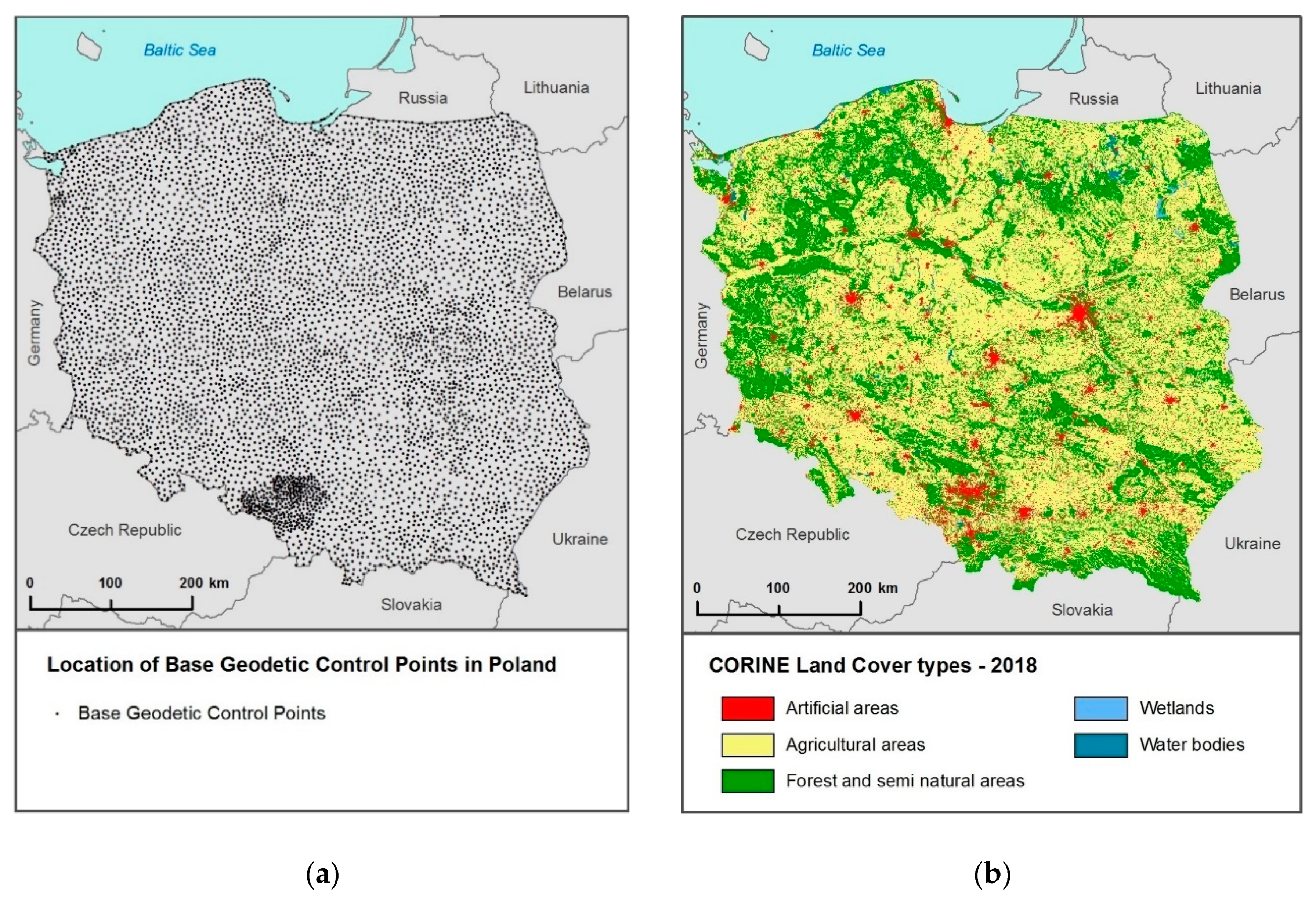
3.1. Area of Investigation and Data Used
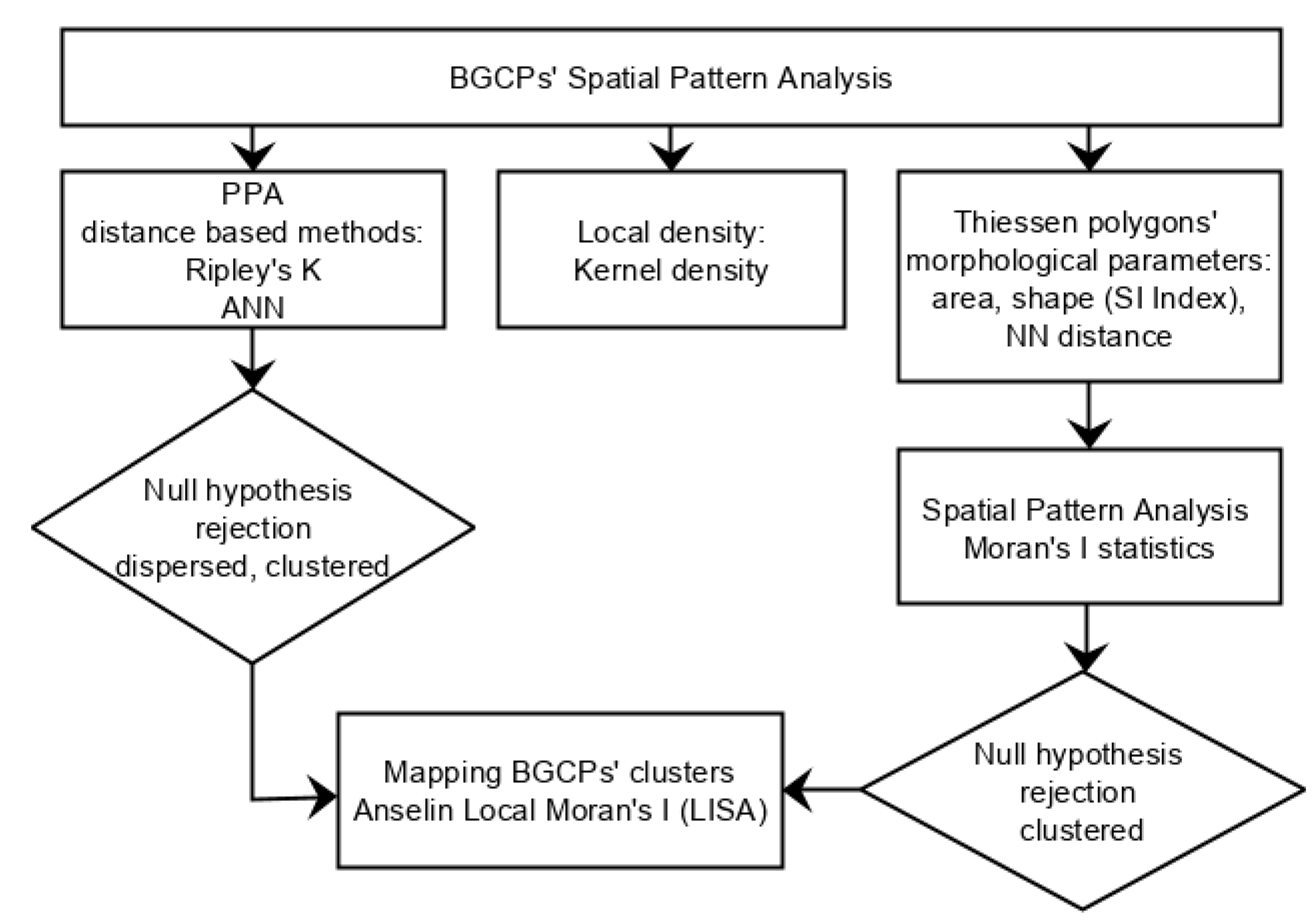
3.2. Research Hypotesis and Methods
3.2.1. Point Pattern Analysis
3.2.2. Thiessen Polygons
3.2.3. Spatial Autocorelation, Cluster and Outlier Analysis
4. Results
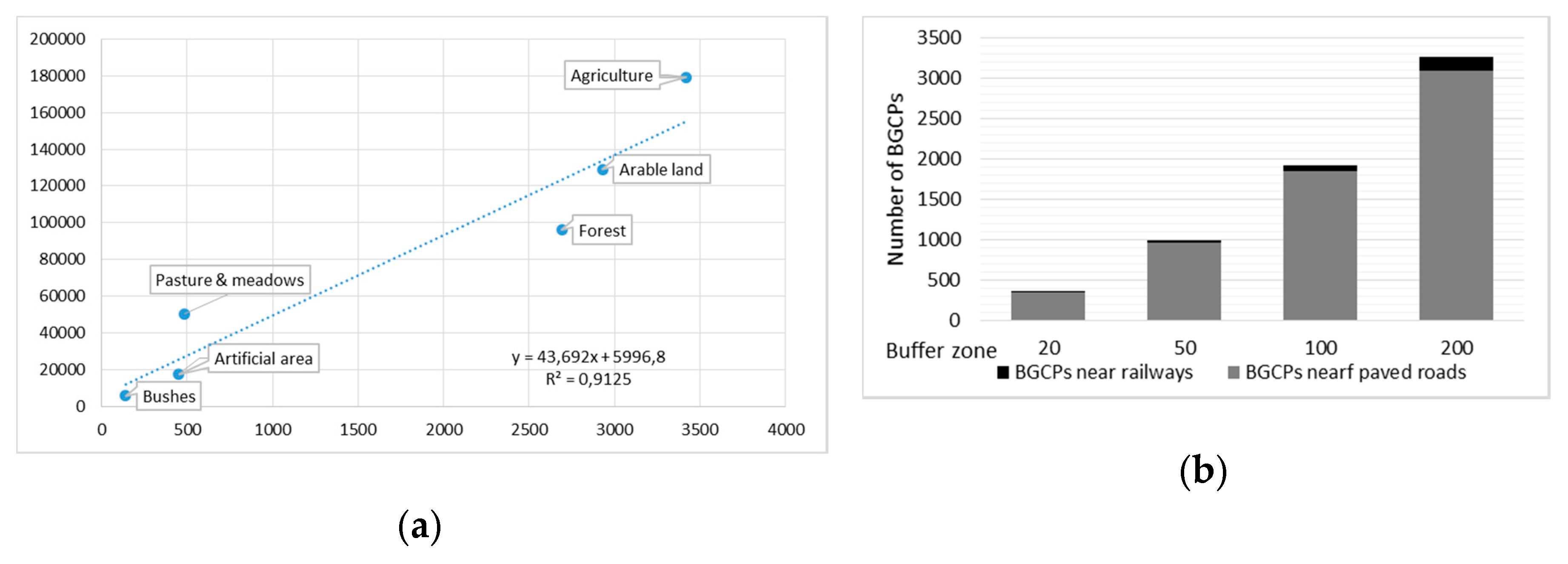
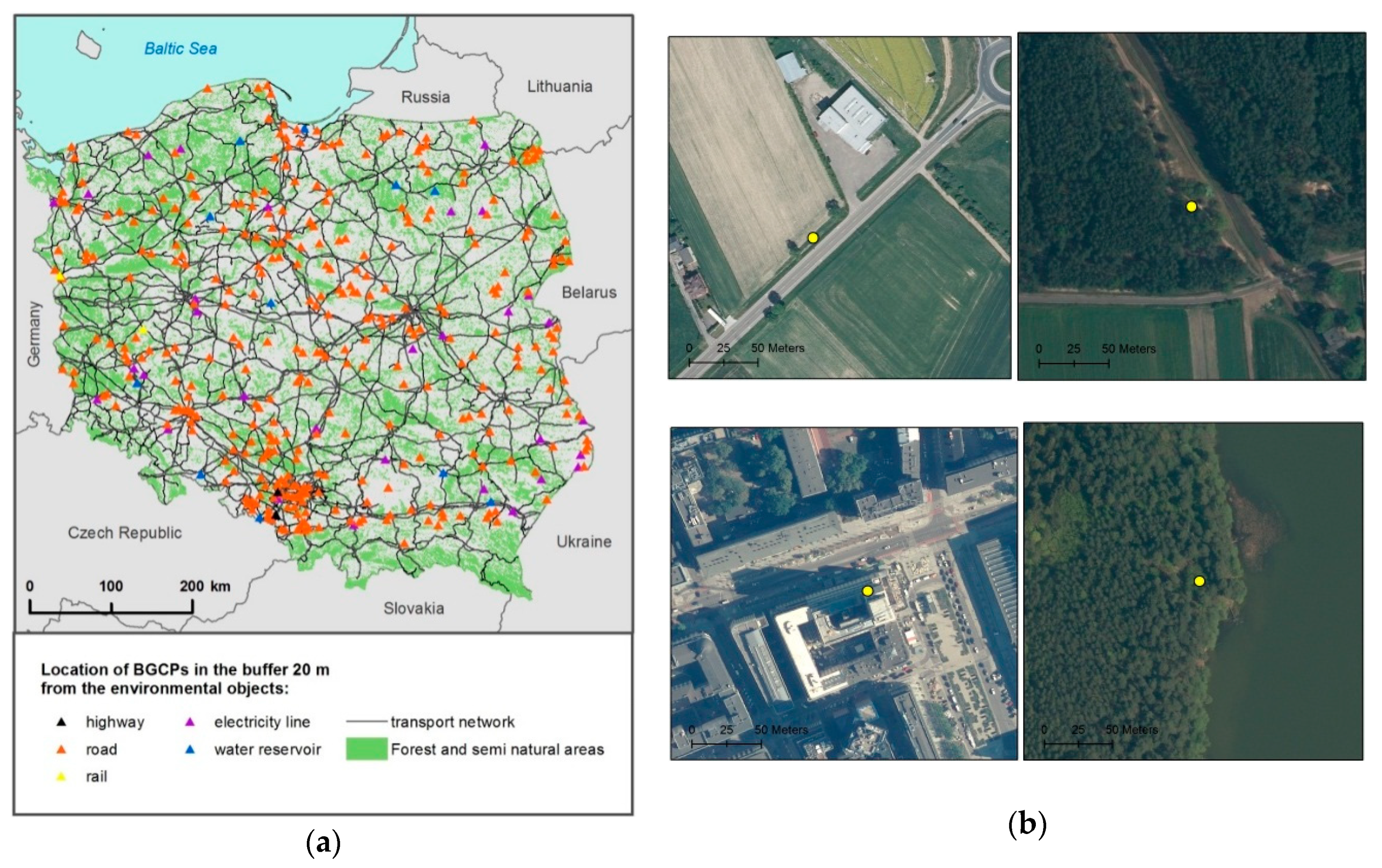
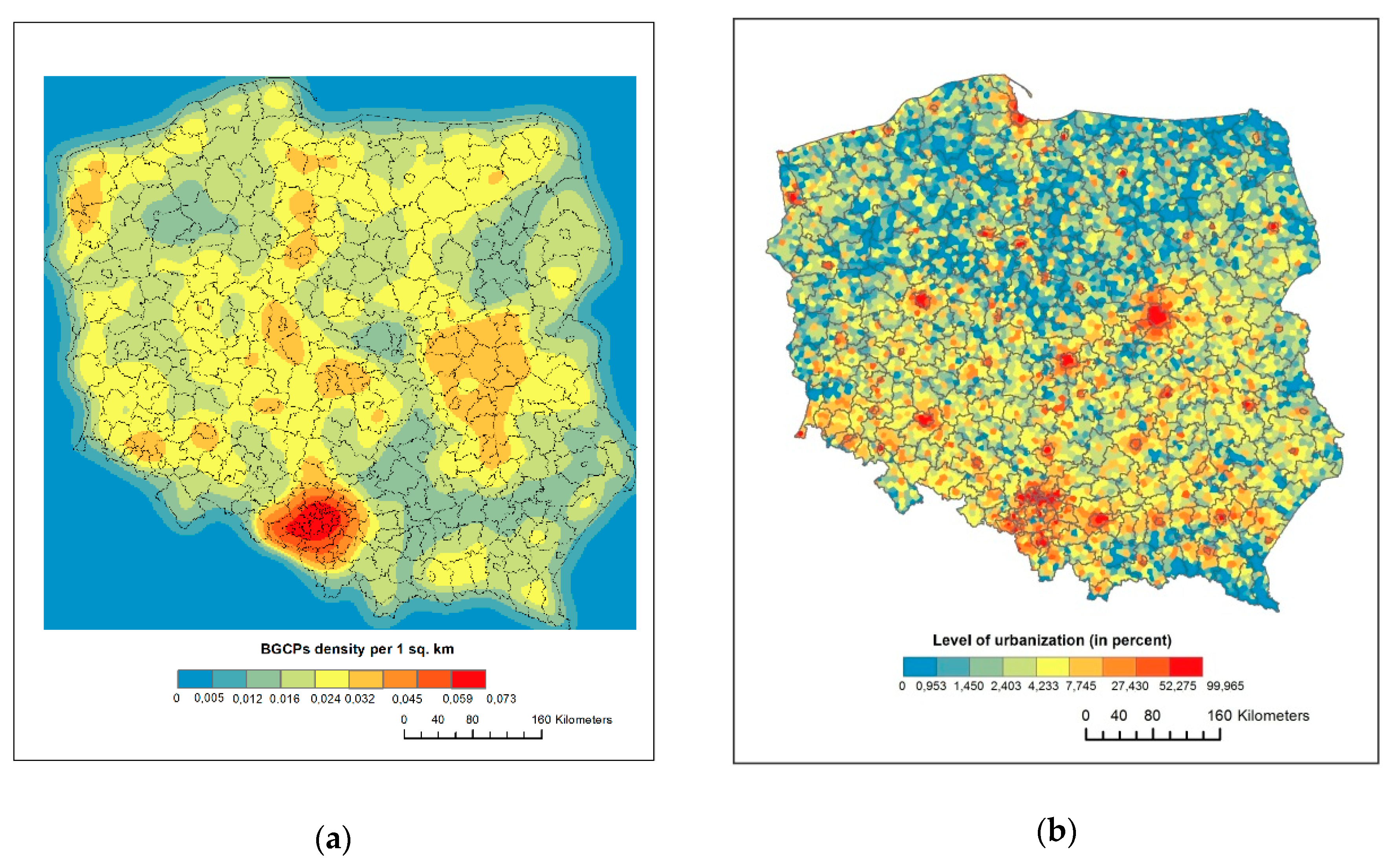
4.1. General Characteristic of BGCPs’ Location
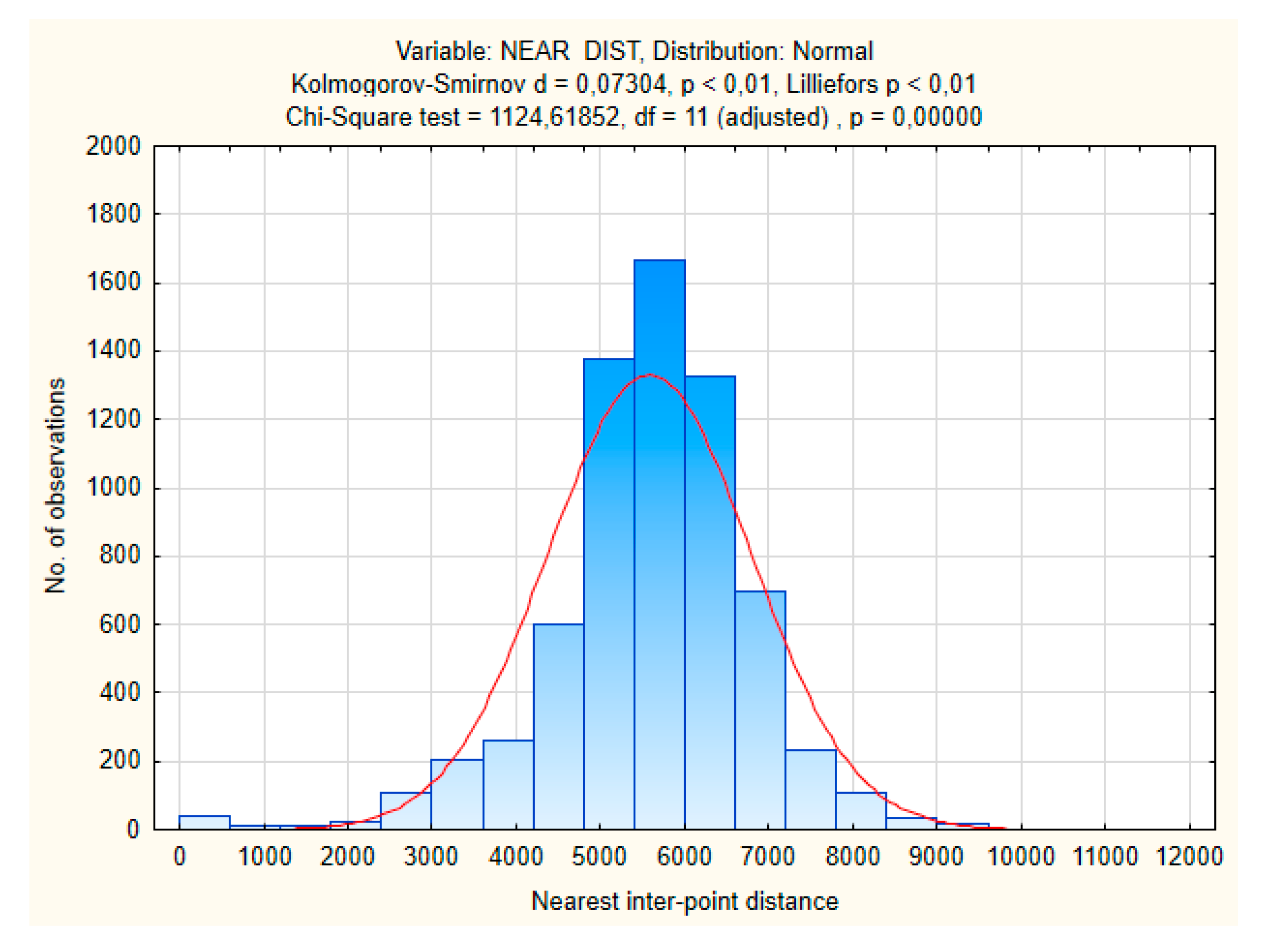
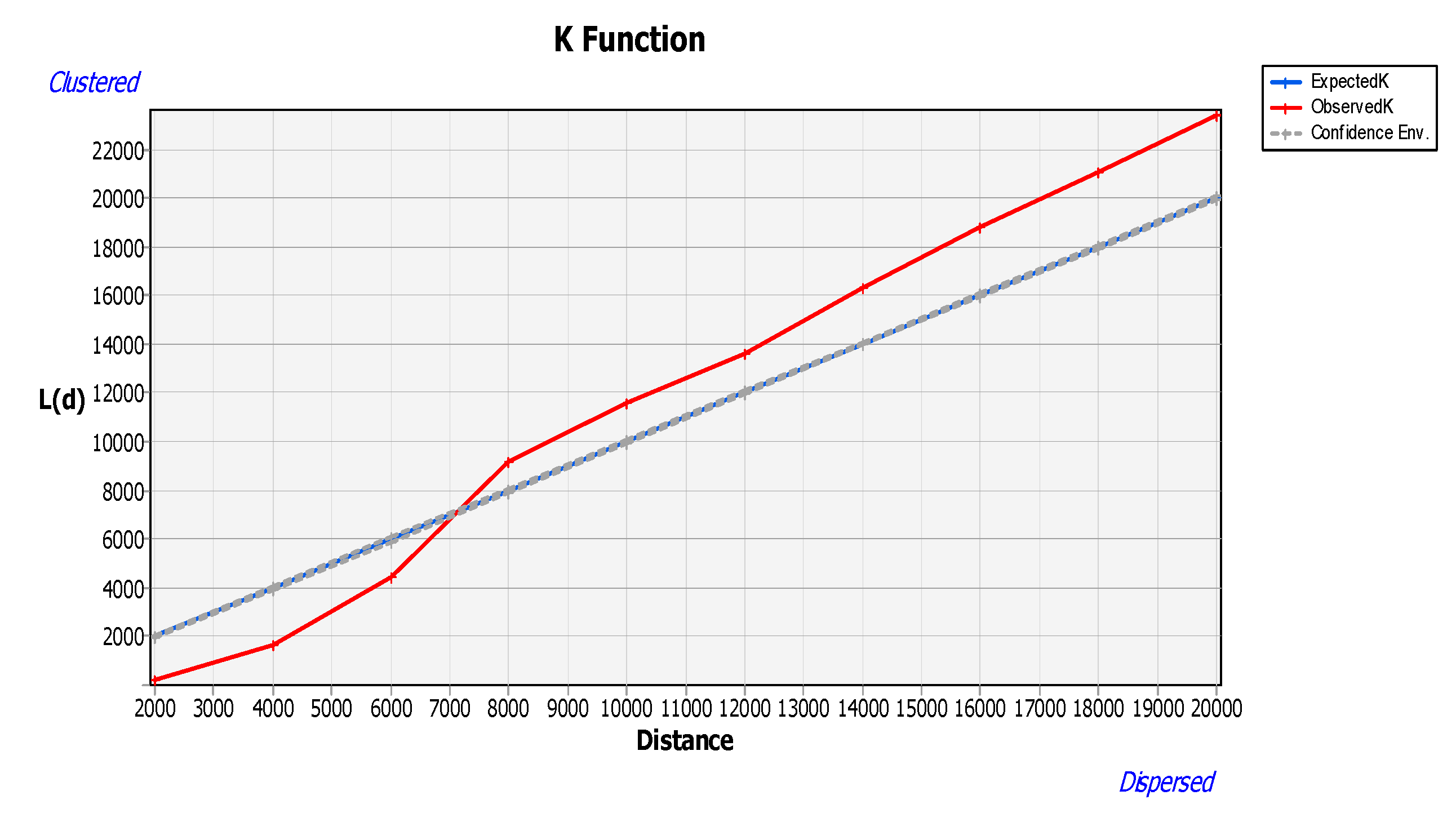
4.2. Point Pattern Analysis
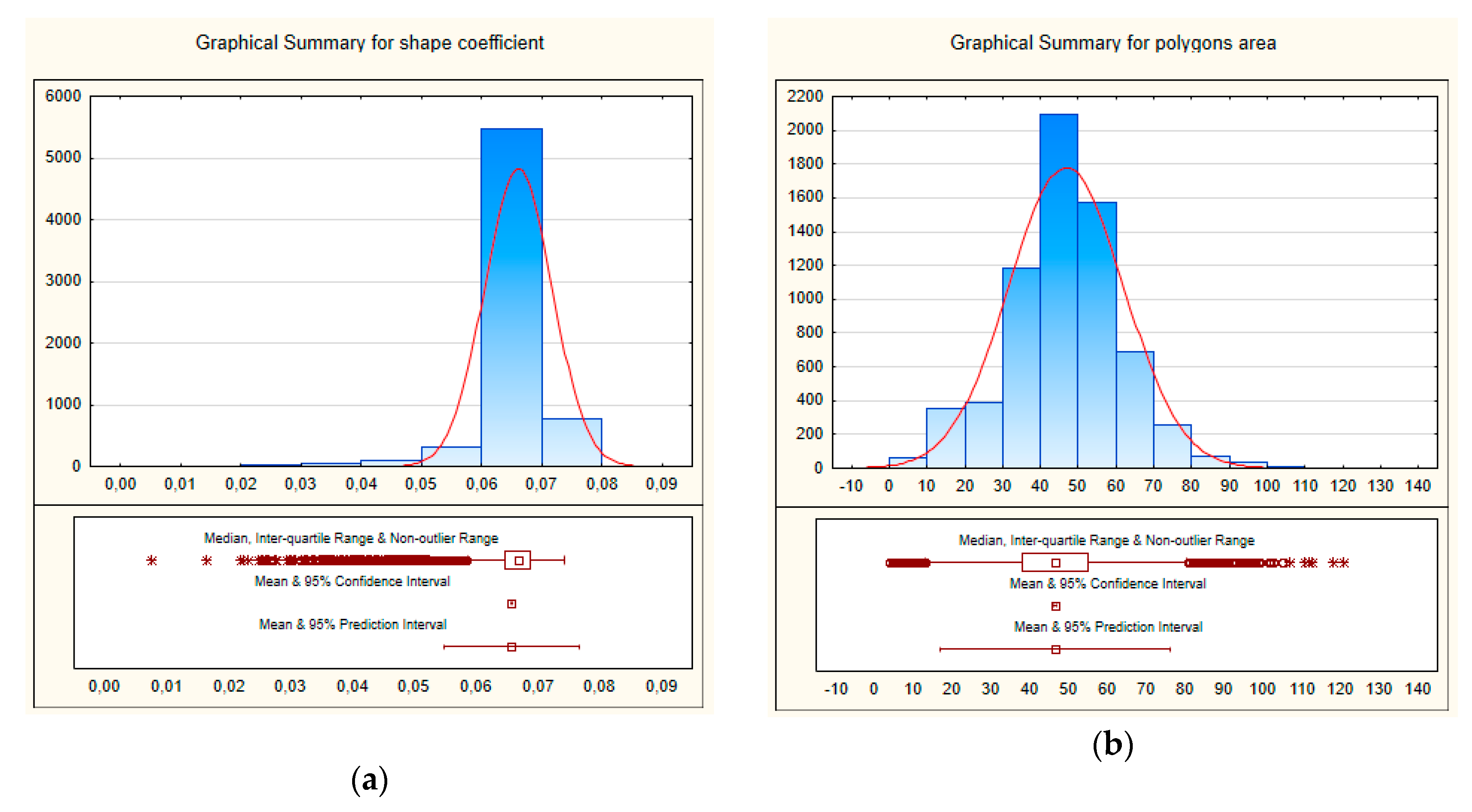
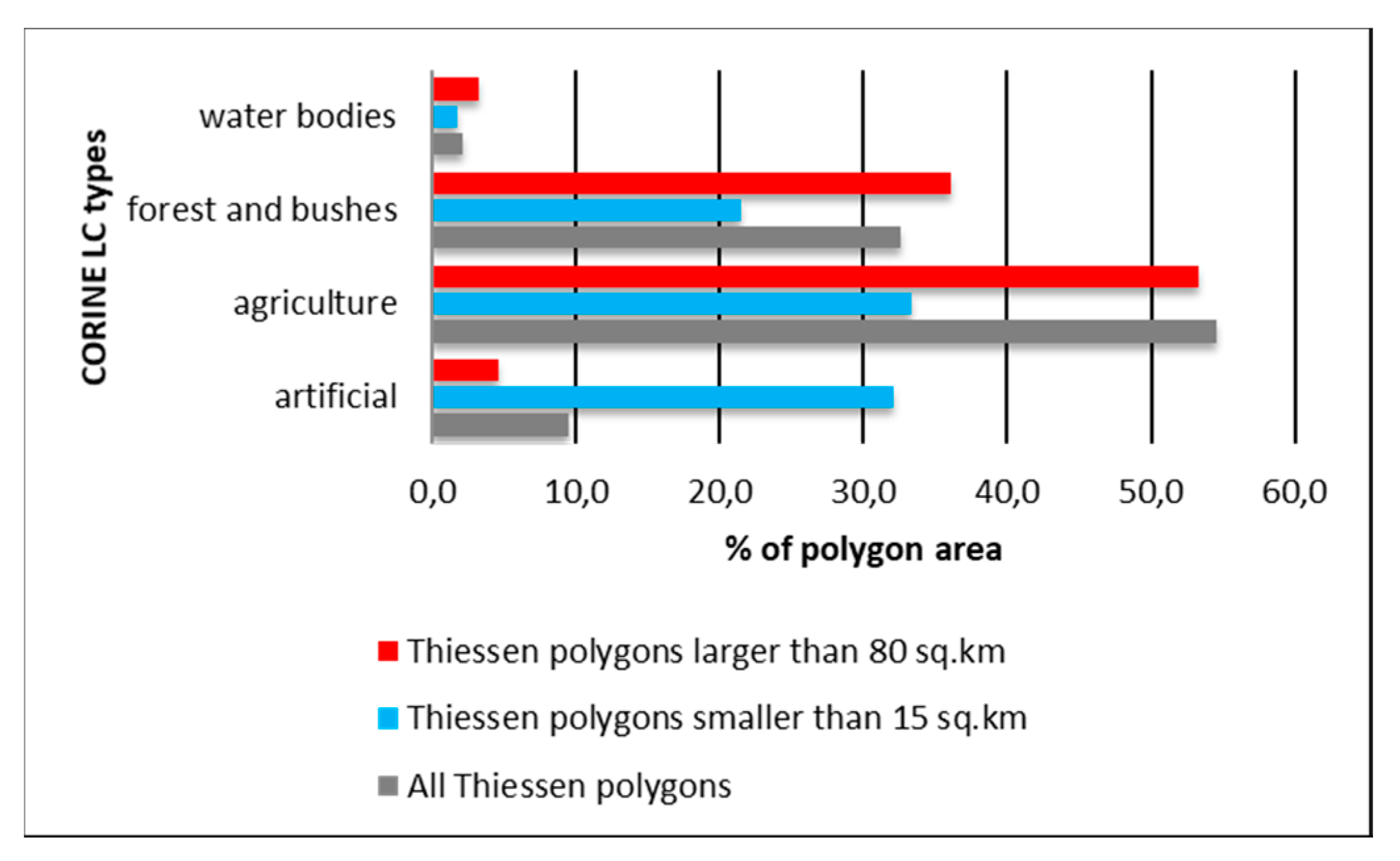
4.3. Thiessen Polygons Morphology and Land Cover Structure
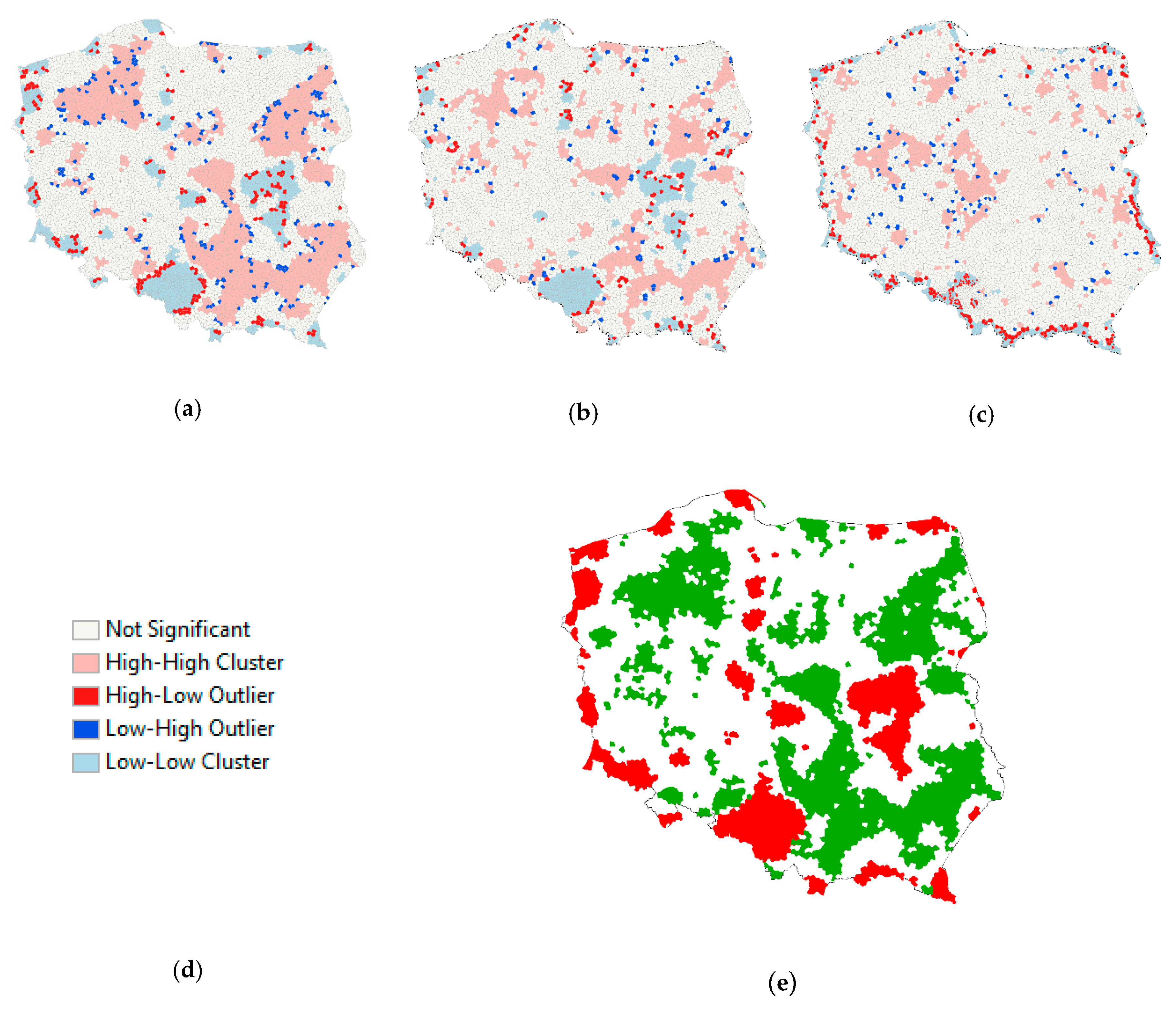
4.4. Quantification of Geodetic Network Uniformity
5. Discussion
6. Conclusions
Author Contributions
Funding
Acknowledgments
Conflicts of Interest
References
- Beutler, G.; Mueller, I.I.; Neilan, R.E. The International GPS Service for Geodynamics: Development and start of official service on January 1, 1994. Bull. Geod. 1994, 68, 39–70. [Google Scholar]
- Kouba, J. Measuring Seismic Waves Induced by Large Earthquakes with GPS. Studia Geophys. Et Geod. 2003, 47, 741–755. [Google Scholar] [CrossRef]
- Głowacki, T. Accuracy analysis of satellite measurements of the measurement geodetic control network on the southern Spitsbergen. E3s Web Conf. 2018, 71, 00020. [Google Scholar] [CrossRef]
- Dalyot, S. Landform Monitoring and Warning Framework Based on Time Series Modeling of Topographic Databases. Geosciences 2015, 5, 177–202. [Google Scholar] [CrossRef] [Green Version]
- Carabajal, C.C.; Harding, D.J.; Suchdeo, V.P. Icesat lidar and global digital elevation models: Applications to desdyni. In Proceedings of the 2010 IEEE International Geoscience and Remote Sensing Symposium, Honolulu, HI, USA, 25–30 July 2010; pp. 1907–1910. [Google Scholar] [CrossRef]
- Bielecka, E.; Maleta, M. Distance Based Synthetic Measure of Agricultural Parcel Locations. Geod. List 2018, 72, 259–276. [Google Scholar]
- Skorupka, D.; Duchaczek, A.; Kowacka, M.; Zagrodnik, P. Quantification of geodetic risk factors occurring at the construction project preparation stage. Arch. Civ. Eng. 2018, 64, 195–200. [Google Scholar] [CrossRef] [Green Version]
- Sabová, J.; Pukanská, K. Expansion of Local Geodetic Point Field and Its Quality/Rozvsírenie Lokálneho Geodetického Bodového Poľa A Jeho Kvalita. Geosci. Eng. 2012, 58, 47–51. [Google Scholar] [CrossRef]
- Gawronek, P.; Makuch, M.; Mitka, B.; Gargula, T. Measurements of the Vertical Displacements of a Railway Bridge Using TLS Technology in the Context of the Upgrade of the Polish Railway Transport. Sensors 2019, 19, 4275. [Google Scholar] [CrossRef] [Green Version]
- Noszczyk, T.; Hernik, J. Modernization of the land and property register. Acta Sci. Pol. Form. Circumiectus 2016, 15, 3–17. [Google Scholar] [CrossRef]
- Mościcka, A.; Kuźma, M. Spatio-Temporal Database of Places Located in the Border Area. ISPRS Int. J. Geo-Inf. 2018, 7, 108. [Google Scholar] [CrossRef] [Green Version]
- Wabiński, J.; Mościcka, A. Natural Heritage Reconstruction Using Full-Color 3D Printing: A Case Study of the Valley of Five Polish Ponds. Sustainability 2019, 11, 5907. [Google Scholar] [CrossRef] [Green Version]
- Janečka, K. The Integrated Management of Information about the Geodetic Point Fields—A Case of the Czech Republic. Geosciences 2019, 9, 307. [Google Scholar] [CrossRef] [Green Version]
- Lisec, A.; Navratil, G. The Austrian land cadastre: From the earliest beginnings to the modern land information system. Geod. Vestn. 2014, 58, 482–516. [Google Scholar] [CrossRef]
- ISO/TC2011/WG7. Final Report from Stage 0 Project on ISO 19152 LADM. Available online: https://isotc.iso.org/livelink/livelink/open/tc211wg7 (accessed on 30 January 2020).
- Bosy, J.; Krynski, J. Reference frames and reference networks. Geod. Cartogr. 2015, 64, 147–176. [Google Scholar] [CrossRef]
- Kadaj, R. The combined geodetic network adjusted on the reference ellipsoid–A comparison of three functional models for GNSS observations. Geod. Cartogr. 2016, 65, 229–257. [Google Scholar] [CrossRef]
- Čada, V.; Janečka, K. Localization of Manuscript Müller’s Maps. Cartogr. J. 2017, 54, 126–138. [Google Scholar] [CrossRef]
- Vera, Y.; Besimbaeva, O.; Khmyrova, E. Analysis of errors in the creation and updating of digital topographic maps. Geod. Cartogr. 2018, 67, 143–151. [Google Scholar] [CrossRef]
- Fryskowska, A.; Wróblewski, P. Mobile Laser Scanning accuracy assessment for the purpose of base-map updating. Geod. Cartogr. 2018, 67, 33–55. [Google Scholar] [CrossRef]
- Kaplan, M.; Ayan, T.; Erol, S. The Effects of Geodetic Configuration of the Network in Deformation Analysis. In Proceedings of the FIG Working Week 2004, Athens, Greece, 22–27 May 2004; Volume 27. Paper Number TS29.6. [Google Scholar]
- Pokonieczny, K.; Calka, B.; Bielecka, E.; Kaminski, P. Modeling Spatial Relationships between Geodetic Control Points and Land Use with Regards to Polish Regulation. In Proceedings of the 2016 Baltic Geodetic Congress (BGC Geomatics), Gdansk, Poland, 2–4 June 2016; pp. 176–180. [Google Scholar] [CrossRef]
- Calka, B.; Bielecka, E.; Figurski, M. Spatial pattern of ASG-EUPOS sites. Open Geosci. 2017, 9, 613–621. [Google Scholar] [CrossRef] [Green Version]
- Klein, I.; Matsuoka, M.T.; Souza, S.F.; Collischonn, C. Design of geodetic networks reliable against multiple outliers. Bol. De Ciências Geodésicas 2012, 18, 480–507. [Google Scholar] [CrossRef] [Green Version]
- Bruyninx, C.; Altamimi, Z.; Caporali, A.; Kenyeres, A.; Legrand, J.; Lidberg, M. Guidelines for EUREF Densifications. Available online: http://www.epncb.oma.be/_documentation/guidelines/Guidelines_for_EUREF_Densifications.pdf (accessed on 30 April 2019).
- Zhang, K.; Liu, G.-J.; Wu, F.; Densley, L.; Retscher, G. An Investigation of the Signal Performance of the Current and Future GNSS in Typical Urban Canyons in Australia Using a High Fidelity 3D Urban Model. In Location Based Services and TeleCartography II: From Sensor Fusion to Context Models; Gartner, G., Rehrl, K., Eds.; Lecture Notes in Geoinformation and Cartography; Springer: Berlin/Heidelberg, Germany, 2009; pp. 407–420. ISBN 978-3-540-87393-8. [Google Scholar]
- Han, J.-Y.; Li, P.-H. Utilizing 3-D topographical information for the quality assessment of a satellite surveying. Appl. Geomat. 2010, 2, 21–32. [Google Scholar] [CrossRef] [Green Version]
- Rapinski, J.; Janowski, A. The Optimal Location of Ground-Based GNSS Augmentation Transceivers. Geosciences 2019, 9, 107. [Google Scholar] [CrossRef] [Green Version]
- Bielecka, E.; Pokonieczny, K.; Kamiński, P. Study on spatial distribution of horizontal geodetic control points in rural areas. Acta Geod. Geop. 2014, 49, 357–368. [Google Scholar] [CrossRef] [Green Version]
- Pokonieczny, K.; Bielecka, E.; Kaminski, P. Analysis of Spatial Distribution of Geodetic Control Points and Land Cover. In Proceedings of the 14th International Multidisciplinary Scientific Geoconference (SGEM) Geoconference on Informatics, Geoinformatics and Remote Sensing, Albena, Bulgaria, 19–25 June 2014; pp. 49–56. [Google Scholar] [CrossRef]
- Pokonieczny, K.; Bielecka, E.; Kamiński, P. Analysis of geodetic control points density depending on the land cover and relief—The Opoczno district case study. In Proceedings of the International Conference on Environmental Engineering ICEE, Vilnius, Lithuania, 27–28 April 2017. [Google Scholar] [CrossRef]
- Regulation of the Ministry of Administration and Digitization, Regarding the Geodetic, Gravimetric and Magnetic Control Networks. Warsaw, 2012; (In Polish). Available online: http://prawo.sejm.gov.pl/isap.nsf/DocDetails.xsp?id=WDU20120000352 (accessed on 9 November 2019).
- Panel on a Multipurpose Cadastre, National Research Council (US). Procedures and Standards for a Multipurpose Cadastre; The National Academies Press: Washington, DC, USA, 1983. [Google Scholar]
- Stanková, H.; Černota, P. A principle of forming and developing geodetic bases in the Czech Republic. Geod. Ir Kartogr. 2010, 36, 103–112. [Google Scholar] [CrossRef]
- Standard for the Australian Survey Control Network Special Publication 1 (SP1), Version 2.1. 2014. Available online: https://www.icsm.gov.au/publications/standard-australian-survey-control-network-special-publication-1-sp1 (accessed on 9 November 2019).
- Federal Geographic Data Committee. Part 4: Geodetic Control. In Geographic Information Framework Data Content Standard; 2008. Available online: https://www.fgdc.gov/standards/projects/framework-data-standard (accessed on 9 November 2019).
- Specht, C.; Skóra, M. Comparative of selected active geodetic networks. Zesz. Nauk. Akad. Mar. Wojennej 2009, XLX, 39–54. (In Polish) [Google Scholar]
- The Geodetic and Cartographic Law; Warsaw, 2019; (In Polish). Available online: http://prawo.sejm.gov.pl/isap.nsf/DocDetails.xsp?id=WDU19890300163 (accessed on 9 November 2019).
- ASG-EUPOS. Available online: http://www.asgeupos.pl/ (accessed on 9 November 2019).
- Doskocz, A. The current state of the creation and modernization of national geodetic and cartographic resources in Poland. Open Geosci. 2016, 8, 579–592. [Google Scholar] [CrossRef]
- Bielecka, E.; Dukaczewski, D.; Janczar, E. Spatial Data Infrastructure in Poland—lessons learnt from so far achievements. Geod. Cartogr. 2018, 67, 3–20. [Google Scholar] [CrossRef]
- International Monetary Fund. World Economic Outlook Database October 2019. Available online: https://www.imf.org/external/pubs/ft/weo/2019/02/weodata/index.aspx (accessed on 9 November 2019).
- Eurostat. Available online: https://ec.europa.eu/eurostat/home? (accessed on 9 November 2019).
- United Nations Development Programme. Human Development Indices and Indicators: 2018 Statistical Update—World 2018; UNDP: New York, NY, USA, 2018. [Google Scholar]
- Statistical Yearbook of the Republic of Poland 2018; GUS: Warsaw, Poland, 2018.
- CORINE Land Cover—Copernicus Land Monitoring Service. Available online: http://land.copernicus.eu/pan-european/corine-land-cover (accessed on 1 October 2017).
- Pokonieczny, K.; Mościcka, A. The Influence of the Shape and Size of the Cell on Developing Military Passability Maps. ISPRS Int. J. Geo-Inf. 2018, 7, 261. [Google Scholar] [CrossRef] [Green Version]
- Ge, Y.; Jin, Y.; Stein, A.; Chen, Y.; Wang, J.; Wang, J.; Cheng, Q.; Bai, H.; Liu, M.; Atkinson, P.M. Principles and methods of scaling geospatial Earth science data. Earth-Sci. Rev. 2019, 197, 102897. [Google Scholar] [CrossRef]
- Cressie, N.; Wikle, C.K. Statistics for Spatio-Temporal Data; Wiley: Hoboken, NJ, USA, 2011; ISBN 978-0-471-69274-4. [Google Scholar]
- Diggle, P.J. Statistical Analysis of Spatial Point Patterns; Academic Press: Cambridge, MA, USA, 1983; ISBN 0-12-215850-4. [Google Scholar]
- Cressie, N. Statistics for Spatial Data, Revised Edition; Wiley Series in Probability and Statistics; John Wiley & Sons Inc.: Hoboken, NJ, USA, 1993; ISBN 978-1-119-11515-1. [Google Scholar]
- Li, F.; Zhang, L. Comparison of point pattern analysis methods for classifying the spatial distributions of spruce-fir stands in the north-east USA. For. Int. J. For. Res. 2007, 80, 337–349. [Google Scholar] [CrossRef] [Green Version]
- Gimond, M. Intro to GIS and Spatial Analysis. 2019. Available online: https://mgimond.github.io/Spatial/index.html (accessed on 15 November 2019).
- Gatrell, A.C.; Bailey, T.C.; Diggle, P.J.; Rowlingson, B.S. Spatial Point Pattern Analysis and Its Application in Geographical Epidemiology. Trans. Inst. Br. Geogr. 1996, 21, 256–274. [Google Scholar] [CrossRef]
- Deng, Y.; Liu, J.; Liu, Y.; Luo, A. Detecting Urban Polycentric Structure from POI Data. ISPRS Int. J. Geo-Inf. 2019, 8, 283. [Google Scholar] [CrossRef] [Green Version]
- Ripley, B.D. The Second-Order Analysis of Stationary Point Processes. J. Appl. Probab. 1976, 13, 255–266. [Google Scholar] [CrossRef] [Green Version]
- Ripley, B.D. Modelling Spatial Patterns. J. R. Stat. Society. Ser. B 1977, 39, 172–212. [Google Scholar] [CrossRef]
- Ripley, B.D. Statistical Inference for Spatial Processes; Cambridge University Press: Cambridge, UK, 1988; ISBN 978-0-521-42420-2. [Google Scholar]
- Mitchell, A. The ESRI Guide to GIS Analysis, Volume 2: Spatial Measurements and Statistics; Esri Press: Redlands, CA, USA, 2005; ISBN 978-1-58948-295-1. [Google Scholar]
- Klein, R. Abstract voronoi diagrams and their applications. In Workshop on Computational Geometry; Noltemeier, H., Ed.; Springer: Berlin/Heidelberg, Germany, 1988; pp. 148–157. [Google Scholar] [CrossRef]
- Chiu, S.N. Spatial Point Pattern Analysis by using Voronoi Diagrams and Delaunay Tessellations—A Comparative Study. Biom. J. 2003, 45, 367–376. [Google Scholar] [CrossRef] [Green Version]
- Zhou, X.; Ding, Y.; Wu, C.; Huang, J.; Hu, C. Measuring the Spatial Allocation Rationality of Service Facilities of Residential Areas Based on Internet Map and Location-Based Service Data. Sustainability 2019, 11, 1337. [Google Scholar] [CrossRef] [Green Version]
- Wang, S.; Sun, L.; Rong, J.; Yang, Z. Transit Traffic Analysis Zone Delineating Method Based on Thiessen Polygon. Sustainability 2014, 6, 1821–1832. [Google Scholar] [CrossRef] [Green Version]
- Krummel, J.R.; Gardner, R.H.; Sugihara, G.; O’Neill, R.V.; Coleman, P.R. Landscape Patterns in a Disturbed Environment. Oikos 1987, 48, 321–324. [Google Scholar] [CrossRef] [Green Version]
- Walker, J.T. Statistics in Criminal Justice: Analysis and Interpretation; Jones & Bartlett Learning: Aspen, CO, USA, 1999; ISBN 978-0-8342-1086-8. [Google Scholar]
- De Smith, M.J.; Goodchild, M.F.; Longley, P. Geospatial Analysis: A Comprehensive Guide to Principles, Techniques and Software Tools; Troubador Publishing Ltd.: Leicester, UK, 2007. [Google Scholar]
- Anselin, L. Local Indicators of Spatial Association—LISA. Geogr. Anal. 1995, 27, 93–115. [Google Scholar] [CrossRef]
- Dembek, W. New Vision of the Role of Land Reclamation Systems in Nature Protection and Water Management. In Wetlands and Water Framework Directive: Protection, Management and Climate Change; Ignar, S., Grygoruk, M., Eds.; GeoPlanet: Earth and Planetary Sciences; Springer International Publishing: Berlin/Heidelberg, Germany, 2015; pp. 91–103. ISBN 978-3-319-13764-3. [Google Scholar]
- Arbia, G. Modelling the geography of economic activities on a continuous space. Pap. Reg. Sci. 2001, 80, 411–424. [Google Scholar] [CrossRef]
- Gutiérrez, A.; Arauzo-Carod, J.-M. Spatial Analysis of Clustering of Foreclosures in the Poorest-Quality Housing Urban Areas: Evidence from Catalan Cities. ISPRS Int. J. Geo-Inf. 2018, 7, 23. [Google Scholar] [CrossRef] [Green Version]
- Preweda, E. Detailed Horizontal Geodetic Control Networks Taking Into Account the Accuracy of the Reference Points. In Proceedings of the 18th International Multidisciplinary Scientific Geoconference (SGEM), Albena, Bulgaria, 17–26 June 2018. [Google Scholar]
- Ślusarski, M.; Justyniak, N. Experimental Evaluation of the Accuracy Parameters of Former Surveying Networks. Infrastrukt. I Ekol. Teren. Wiej. 2017, 2, 825–835. [Google Scholar] [CrossRef]
- Schmitt, G. Review of Network Designs: Criteria, Risk Functions, Design Ordering. In Optimization and Design of Geodetic Networks; Grafarend, E.W., Sansò, F., Eds.; Springer: Berlin/Heidelberg, Germany, 1985; pp. 6–10. [Google Scholar]
- Wanninger, L. Real-Time Differential GPS Error Modelling in Regional Reference Station Networks. In Advances in Positioning and Reference Frames; Brunner, F.K., Ed.; Springer: Berlin/Heidelberg, Germany, 1998; pp. 86–92. [Google Scholar] [CrossRef]
- Lee, I.-S.; Ge, L. The performance of RTK-GPS for surveying under challenging environmental conditions. Earthplanets Space 2006, 58, 515–522. [Google Scholar] [CrossRef] [Green Version]
- Goodchild, M.F. Scale in GIS: An overview. Geomorphology 2011, 130, 5–9. [Google Scholar] [CrossRef]
- Goodchild, M.F. Formalizing Place in Geographic Information Systems. In Communities, Neighborhoods, and Health: Expanding the Boundaries of Place; Burton, L.M., Matthews, S.A., Leung, M., Kemp, S.P., Takeuchi, D.T., Eds.; Social Disparities in Health and Health Care; Springer: New York, NY, USA, 2011; pp. 21–33. ISBN 978-1-4419-7482-2. [Google Scholar]
- Steudler, D.; Rajabifard, A.; Williamson, I.P. Evaluation of land administration systems. Land Use Policy 2004, 21, 371–380. [Google Scholar] [CrossRef] [Green Version]


| Data Set | Abbreviation | CRS 1 | Data Format | Date | Data Provider |
|---|---|---|---|---|---|
| Base National Geodetic Network | BNGN | ETRS89 | txt | 2016 | Central Geodetic and Cartographic Documentation Centre |
| CORINE Land Cover | CLC | ETRS89 | shape | 2018 | Copernicus Land Monitoring Service |
| Vector Smart Map level 2 | VmapL2 | WGS84 | VPF | 2018 | Polish Military Geography Directorate |
| CORINE Land Cover Types | Number of BGCPs (Frequency) | Area [km2] | Density BGCPs/1km2 | Density BGCPs/50 km2 |
|---|---|---|---|---|
| Artificial area | 452 | 17,605 | 0.026 | 1.284 |
| Agriculture, including: | 3417 | 179,307 | 0.019 | 0.953 |
| Arable land | 2931 | 128,966 | 0.023 | 1.136 |
| Pastures and meadows | 486 | 50,341 | 0.010 | 0.483 |
| Forest | 2692 | 96,209 | 0.028 | 1.399 |
| Bushes | 141 | 5669 | 0.025 | 1.243 |
| Others (e.g., bare rock, dispersed vegetation) | 21 | 6701 | 0.003 | 0.157 |
| Poland | 6723 | 312,544 | 0.022 | 1.076 |
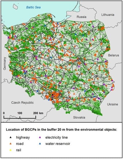
| The Buffer Zone [m] | Number of BGCPs Near Roads | Number of BGCPs Near Railways | Number of BGCPs Near Water Bodies | Number of BGCPs Near Electricity Lines |
|---|---|---|---|---|
| 10 | 157 | 0 | 2 | 19 |
| 20 | 343 | 2 | 5 | 33 |
| 50 | 966 | 22 | 15 | 103 |
| 100 | 1853 | 69 | 60 | 215 |
| 200 | 3094 | 168 | 219 | 474 |
| total | 6256 | 261 | 301 | 844 |
| Variables | Mean | Median | Minimum | Maximum | Range | Quartile (Range) | Variance | Std. Dev. | Coef. Var. [%] |
|---|---|---|---|---|---|---|---|---|---|
| Thiessen polygons area in km2 | 46.480 | 46.636 | 3.685 | 120.806 | 117.120 | 16.881 | 227.271 | 15.076 | 32.434 |
| Shape index of Thiessen polygons | 0.826 | 0.840 | 0.095 | 0.935 | 0.840 | 0.004 | 0.005 | 0.070 | 8.450 |
| Heavily urbanized [%] | 6.65 | 3.32 | 0.00 | 99.96 | 99.96 | 5.23 | 122.22 | 11.05 | 166.16 |
| Sparsely urbanized [%] | 2.79 | 1.70 | 0.00 | 37.11 | 37.11 | 3.22 | 11.97 | 3.46 | 123.97 |
| Agriculture [%] | 53.40 | 57.51 | 0.00 | 99.90 | 99.95 | 39.10 | 650.53 | 25.51 | 47.76 |
| Forest and bushes [%] | 32.45 | 26.52 | 0.00 | 99.98 | 99.98 | 35.64 | 613.72 | 24.77 | 76.35 |
| Water bodies [%] | 2.13 | 0.00 | 0.00 | 97.54 | 97.54 | 1.88 | 36.78 | 6.06 | 285.18 |
| NC | 8.94 | 9.00 | 1.00 | 16.00 | 15.00 | 2.00 | 3.60 | 1.90 | 21.23 |
| NP | 33.90 | 32.00 | 1.00 | 109.00 | 108.00 | 19.00 | 232.67 | 15.25 | 44.99 |
| BGN Regularity Type | RT | RD |
|---|---|---|
| Number of Thiessen polygons | 1504 | 1130 |
| Area in km2 (in %) | 92,643.9 (29.7) | 30,920.1 (9.9) |
| Thiessen polygons min area in km2 | 9.29 | 3.68 |
| Thiessen polygons max area in km2 | 120.80 | 46.44 |
| Thiessen polygons mean area in km2 | 61.60 | 27.26 |
| Thiessen polygons area frequency distribution |  |  |
| NN distance mean value in m | 6789 | 3770 |
© 2020 by the authors. Licensee MDPI, Basel, Switzerland. This article is an open access article distributed under the terms and conditions of the Creative Commons Attribution (CC BY) license (http://creativecommons.org/licenses/by/4.0/).
Share and Cite
Bielecka, E.; Pokonieczny, K.; Borkowska, S. GIScience Theory Based Assessment of Spatial Disparity of Geodetic Control Points Location. ISPRS Int. J. Geo-Inf. 2020, 9, 148. https://0-doi-org.brum.beds.ac.uk/10.3390/ijgi9030148
Bielecka E, Pokonieczny K, Borkowska S. GIScience Theory Based Assessment of Spatial Disparity of Geodetic Control Points Location. ISPRS International Journal of Geo-Information. 2020; 9(3):148. https://0-doi-org.brum.beds.ac.uk/10.3390/ijgi9030148
Chicago/Turabian StyleBielecka, Elzbieta, Krzysztof Pokonieczny, and Sylwia Borkowska. 2020. "GIScience Theory Based Assessment of Spatial Disparity of Geodetic Control Points Location" ISPRS International Journal of Geo-Information 9, no. 3: 148. https://0-doi-org.brum.beds.ac.uk/10.3390/ijgi9030148