Insights into the Structural Requirements of Potent Brassinosteroids as Vegetable Growth Promoters Using Second-Internode Elongation as Biological Activity: CoMFA and CoMSIA Studies


Abstract
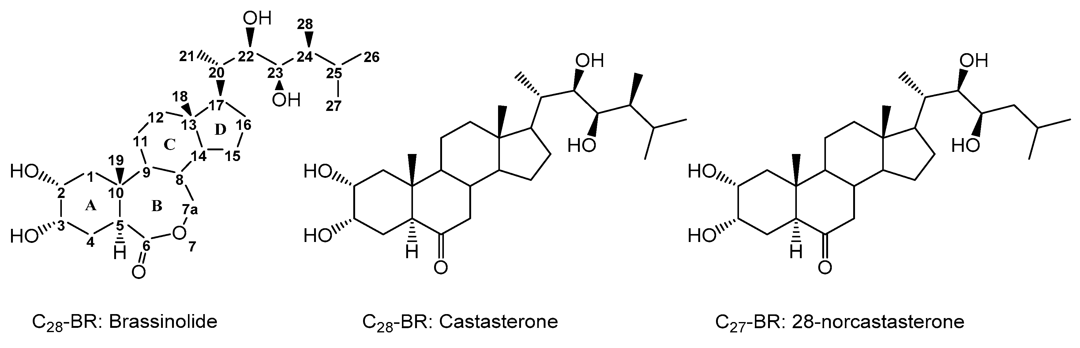
:1. Introduction
2. Results
2.1. Statistical Results of Comparative Molecular Field Analysis (CoMFA) and Comparative Molecular Similarity Indices Analysis (CoMSIA)
2.1.1. CoMFA Statistics
2.1.2. CoMSIA Statistics
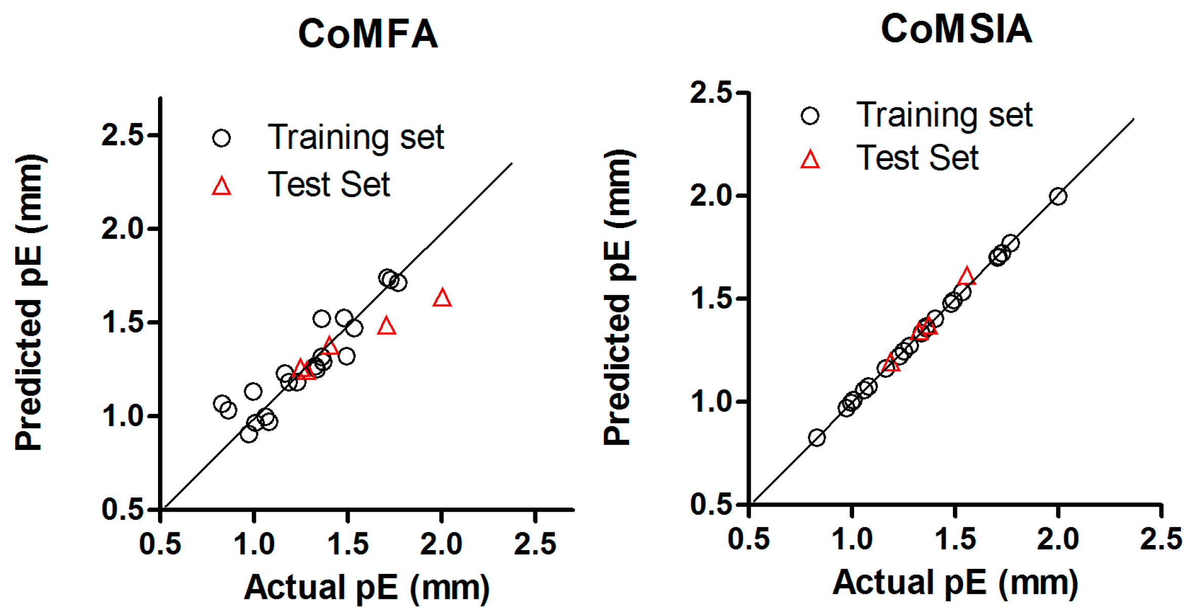
2.2. Validation of the 3D-QSAR Models
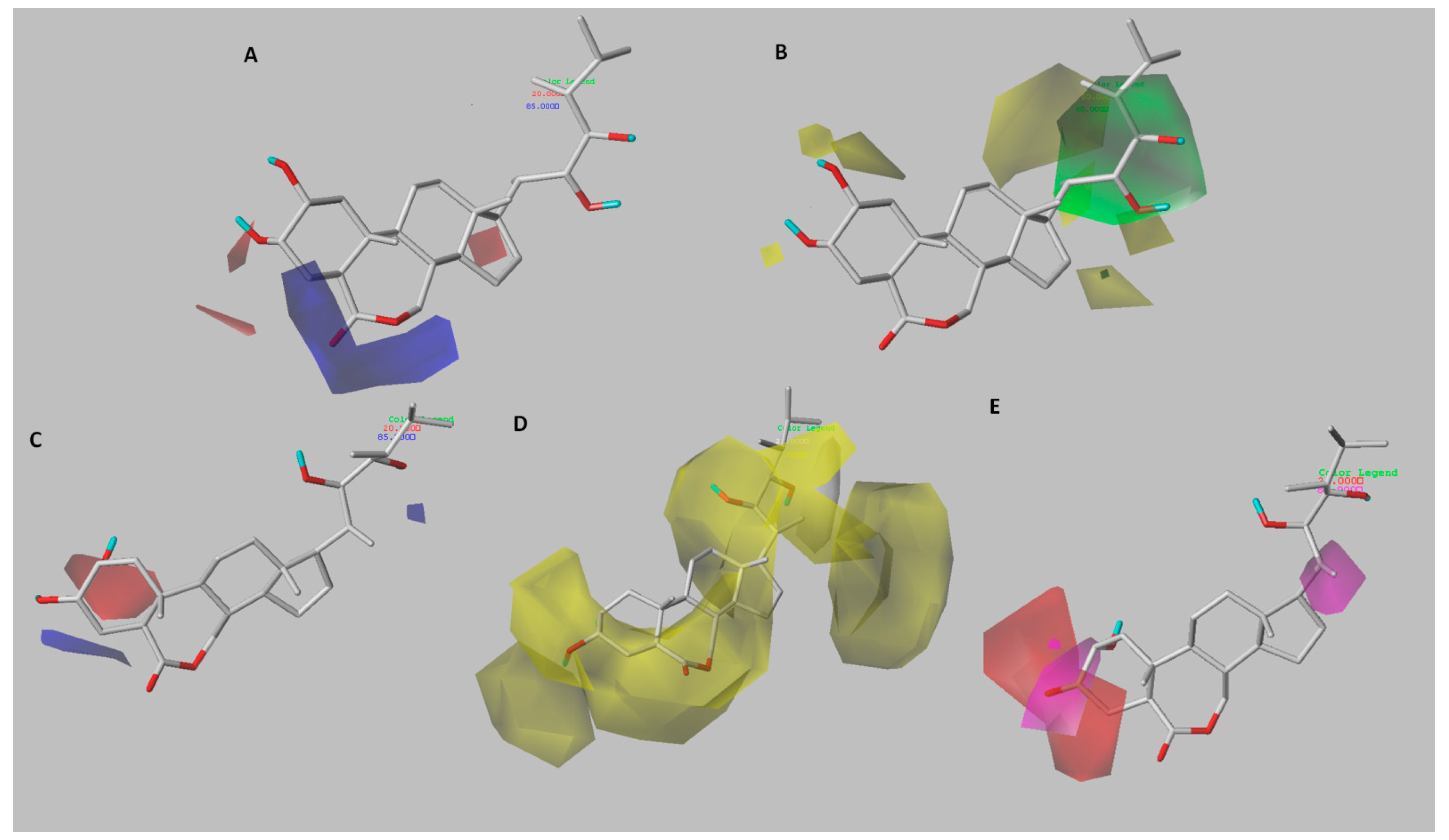
2.3. 3D-QSAR Contour Maps
3. Discussion
3.1. Analysis of CoMFA Contour Maps
3.1.1. Model A
3.1.2. Model B
3.2. Analysis of CoMSIA Contour Maps
3.2.1. Model A
3.2.2. Model B
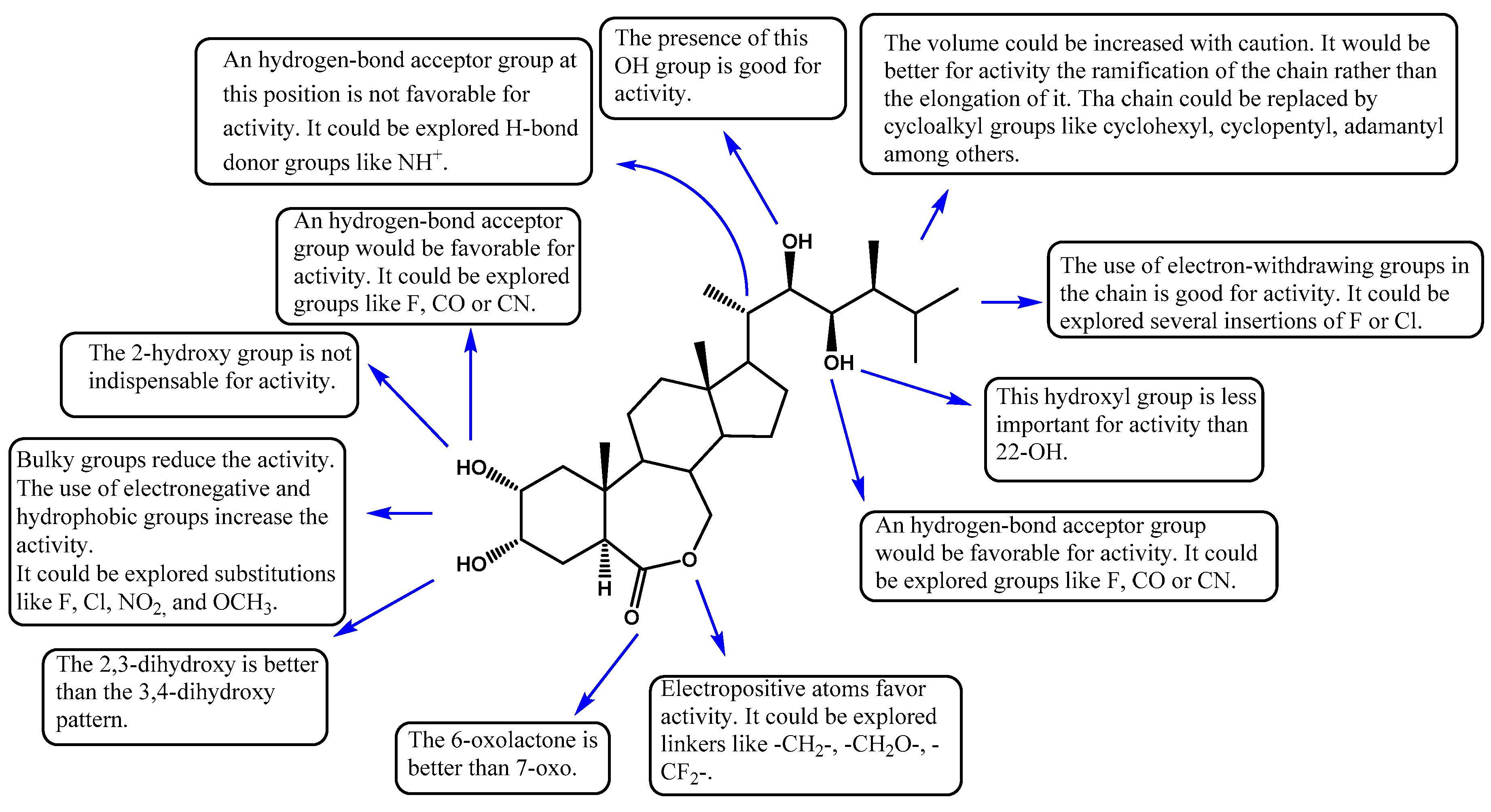
3.2.3. SAR Summary
4. Materials and Methods
4.1. Data Sets Selection and Biological Activity
4.2. Molecular Alignment
4.3. CoMFA and CoMSIA Field Calculation
4.4. Internal Validation and Partial Least Squares (PLS) Analysis
4.5. 3D-QSAR External Validation
5. Conclusions
Acknowledgments
Author Contributions
Conflicts of Interest
Abbreviations
| 3D-QSAR | Three-Dimensional Quantitative Structure–Activity Relationship |
| CoMFA | Comparative Molecular Field Analysis |
| CoMSIA | Comparative Molecular Similarity Index Analysis |
| PLS | Partial Least Squares |
| LOO | Leave-One-Out |
| N | Optimal Number of Components |
| rncv2 | Non-Cross Validation Coefficient |
| q2 | Cross Validation Coefficient |
| r2pred | Predictive Correlation Coefficient |
| F | Fischer-Test Value |
| SEE | Standard Error of Estimation |
| SEP | Standard Error of Prediction |
References
- Vert, G.; Nemhauser, J.L.; Geldner, N.; Hong, F.; Chory, J. Molecular mechanisms of steroid hormone signaling in plants. Annu. Rev. Cell Dev. Biol. 2005, 21, 177–201. [Google Scholar] [CrossRef] [PubMed]
- Izumi, Y.; Okazawa, A.; Bamba, T.; Kobayashi, A.; Fukusaki, E. Development of a method for comprehensive and quantitative analysis of plant hormones by highly sensitive nanoflow liquid chromatography–electrospray ionization-ion trap mass spectrometry. Anal. Chim. Acta 2009, 648, 215–225. [Google Scholar] [CrossRef] [PubMed]
- Kvasnica, M.; Oklestkova, J.; Bazgier, V.; Rarova, L.; Berka, K.; Strnad, M. Biological activities of new monohydroxylated brassinosteroid analogues with a carboxylic group in the side chain. Steroids 2014, 85, 58–64. [Google Scholar] [CrossRef] [PubMed]
- Bajguz, A.; Tretyn, A. The chemical characteristic and distribution of brassinosteroids in plants. Phytochemistry 2003, 62, 1027–1046. [Google Scholar] [CrossRef]
- Bajguz, A.; Tretyn, A. The Chemical Structures and Occurrence of Brassinosteroids in Plants. In Brassinosteroids; Springer: Dordrecht, The Netherlands, 2003; pp. 1–44. [Google Scholar]
- Serna, M.; Hernández, F.; Coll, F.; Amorós, A. Brassinosteroid analogues effect on yield and quality parameters of field-grown lettuce (Lactuca sativa L.). Sci. Hortic. (Amsterdam) 2012, 143, 29–37. [Google Scholar] [CrossRef]
- Acebedo, S.L.; Alonso, F.; Ramírez, J.A.; Galagovsky, L.R. Synthesis of aromatic stigmastanes: Application to the synthesis of aromatic analogs of brassinosteroids. Tetrahedron 2012, 68, 3685–3691. [Google Scholar] [CrossRef]
- Krishna, P. Brassinosteroid-mediated stress responses. J. Plant Growth Regul. 2003, 22, 289–927. [Google Scholar] [CrossRef] [PubMed]
- Bajguz, A.; Piotrowska-Niczyporuk, A. Brassinosteroids Implicated in Growth and Stress Responses. In Phytohormones: A Window to Metabolism, Signaling and Biotechnological Applications; Springer: New York, NY, USA, 2014; pp. 163–190. [Google Scholar]
- Kim, T.-W.; Lee, S.M.; Joo, S.-H.; Yun, H.S.; Lee, Y.; Kaufman, P.B.; Kirakosyan, A.; Kim, S.-H.; Nam, K.H.; Lee, J.S.; et al. Elongation and gravitropic responses of Arabidopsis roots are regulated by brassinolide and IAA. Plant Cell Environ. 2007, 30, 679–689. [Google Scholar] [CrossRef] [PubMed]
- Wang, Q.; Xu, J.; Liu, X.; Gong, W.; Zhang, C. Synthesis of brassinosteroids analogues from laxogenin and their plant growth promotion. Nat. Prod. Res. 2015, 29, 149–157. [Google Scholar] [CrossRef] [PubMed]
- Vlašánková, E.; Kohout, L.; Klemš, M.; Eder, J.; Reinöhl, V.; Hradilík, J. Evaluation of biological activity of new synthetic brassinolide analogs. Acta Physiol. Plant. 2009, 31, 987–993. [Google Scholar] [CrossRef]
- Seto, H.; Hiranuma, S.; Fujioka, S.; Koshino, H.; Suenaga, T.; Yoshida, S. Preparation, conformational analysis, and biological evaluation of 6a-carbabrassinolide and related compounds. Tetrahedron 2002, 58, 9741–9749. [Google Scholar] [CrossRef]
- Back, T.G.; Pharis, R.P. Structure-activity studies of brassinosteroids and the search for novel analogues and mimetics with improved bioactivity. J. Plant Growth Regul. 2003, 22, 350–361. [Google Scholar] [CrossRef] [PubMed]
- Takatsuto, S.; Ikekawa, N.; Morishita, T.; Abe, H. Structure-activity relationship of brassinosteroids with respect to the A/B-ring functional groups. Chem. Pharm. Bull. (Tokyo) 1987, 35, 211–216. [Google Scholar] [CrossRef]
- Brosa, C.; Capdevila, J.M.; Zamora, I. Brassinosteroids: A new way to define the structural requirements. Tetrahedron 1996, 52, 2435–2448. [Google Scholar] [CrossRef]
- Brosa, C.; Zamora, I.; Terricabras, E.; Soca, L.; Peracaula, R.; Rodríguez-Santamarta, C. Synthesis and molecular modeling: Related approaches to progress in brassinosteroid research. Lipids 1997, 32, 1341–1347. [Google Scholar] [CrossRef] [PubMed]
- Brosa, C.; Soca, L.; Terricabras, E.; Ferrer, J.C.; Alsina, A. New synthetic brassinosteroids: A 5α-hydroxy-6-ketone analog with strong plant growth promoting activity. Tetrahedron 1998, 54, 12337–12348. [Google Scholar] [CrossRef]
- Brosa, C.; Zamora, I.; Terricabras, E.; Kohout, L. The Effect of electrostatic properties and abibility to form hydrogen-bonds on the activity of brassinosteroid side-chain analogs. Collect. Czechoslov. Chem. Commun. 1998, 63, 1635–1645. [Google Scholar] [CrossRef]
- Hothorn, M.; Belkhadir, Y.; Dreux, M.; Dabi, T.; Noel, J.P.; Wilson, I.A.; Chory, J. Structural basis of steroid hormone perception by the receptor kinase BRI1. Nature 2011, 474, 467–471. [Google Scholar] [CrossRef] [PubMed]
- She, J.; Han, Z.; Kim, T.-W.; Wang, J.; Cheng, W.; Chang, J.; Shi, S.; Wang, J.; Yang, M.; Wang, Z.-Y.; et al. Structural insight into brassinosteroid perception by BRI1. Nature 2011, 474, 472–476. [Google Scholar] [CrossRef] [PubMed]
- Golbraikh, A.; Tropsha, A. Beware of q2! J. Mol. Graph. Model. 2002, 20, 269–276. [Google Scholar] [CrossRef]
- Pereira-Netto, A.B.; Schaefer, S.; Galagovsky, L.R.; Ramirez, J.A. Brassinosteroid-Driven Modulation of Stem Elongation and Apical Dominance: Applications in Micropropagation. In Brassinosteroids; Hayat, S., Ahmad, A., Eds.; Springer: Dordrecht, The Netherlands, 2003; pp. 129–157. [Google Scholar]
- Baron, D.L.; Luo, W.; Janzen, L.; Pharis, R.P.; Back, T.G. Structure-activity studies of brassinolide B-ring analogues. Phytochemistry 1998, 49, 1849–1858. [Google Scholar] [CrossRef]
- Strnad, M.; Kohout, L. A simple brassinolide analogue 2α, 3α-dihydroxy-17β-(3-methyl-butyryloxy)-7-oxa-B-homo-5α-androstan-6-one which induces bean second internode splitting. Plant Growth Regul. 2003, 40, 39–47. [Google Scholar] [CrossRef]
- Thompson, M.J.; Meudt, W.J.; Mandava, N.B.; Dutky, S.R.; Lusby, W.R.; Spaulding, D.W. Synthesis of brassinosteroids and relationship of structure to plant growth-promoting effects. Steroids 1982, 39, 89–105. [Google Scholar] [CrossRef]
- Takatsuto, S.; Yazawa, N.; Ikekawa, N.; Takematsu, T.; Takeuchi, Y.; Koguchi, M. Structure-activity relationship of brassinosteroids. Phytochemistry 1983, 22, 2437–2441. [Google Scholar] [CrossRef]
- Šíša, M.; Vilaplana-Polo, M.; Ballesteros, C.B.; Kohout, L. Brassinolide activities of 2α,3α-diols versus 3α,4α-diols in the bean second internode bioassay: Explanation by molecular modeling methods. Steroids 2007, 72, 740–750. [Google Scholar] [CrossRef] [PubMed]
- Šíša, M.; Buděšínský, M.; Kohout, L. Synthesis and biological activity of 7a-homo- and 7a,7b-dihomo-5α-cholestane analogues of brassinolide. Collect. Czechoslov. Chem. Commun. 2003, 68, 2171–2189. [Google Scholar] [CrossRef]
- Slavikova, B.; Kohout, L.; Budesinsky, M.; Swaczynova, J.; Kasal, A. Brassinosteroids: Synthesis and activity of some fluoro analogues. J. Med. Chem. 2008, 51, 3979–3984. [Google Scholar] [CrossRef] [PubMed]
- Takatsuto, S.; Yazawa, N.; Ikekawa, N. Synthesis and biological activity of brassinolide analogues, 26,27-bisnorbrassinolide and its 6-oxo analogue. Phytochemistry 1984, 23, 525–528. [Google Scholar] [CrossRef]
- Kohout, L.; Strnad, M. Brassinolide analogues without side chain. Collect. Czechoslov. Chem. Commun. 1989, 54, 1019–1027. [Google Scholar] [CrossRef]
- Zullo, M.A.T.; de Azevedo, M.D.B.M. Brassinosteroids and Brassinosteroid Analogues Inclusion Complexes in Cyclodextrins. In Brassinosteroids; Hayat, S., Ahmad, A., Eds.; Springer: Dordrecht, The Netherlands, 2003; pp. 171–188. [Google Scholar]
- Šíša, M.; Hniličková, J.; Swaczynová, J.; Kohout, L. Syntheses of new androstane brassinosteroids with 17β-ester groups—Butyrates, heptafluorobutyrates, and laurates. Steroids 2005, 70, 755–762. [Google Scholar] [CrossRef] [PubMed]
- Kohout, L.; Velgová, H.; Strnad, M.; Kamínek, M. Brassino steroids with androstane and pregnane skeleton. Collect. Czechoslov. Chem. Commun. 1987, 52, 476–486. [Google Scholar] [CrossRef]
- SYBYL-X 1.2. Tripos International, 1699 South Hanley Rd., St. Louis, Missouri, 63144, USA. 2011.
- Vinter, J.G.; Davis, A.; Saunders, M.R. Strategic approaches to drug design. I. An integrated software framework for molecular modelling. J. Comput. Aided Mol. Des. 1987, 1, 31–51. [Google Scholar] [CrossRef] [PubMed]
- Gasteiger, J.; Marsili, M. Iterative partial equalization of orbital electronegativity—A rapid access to atomic charges. Tetrahedron 1980, 36, 3219–3228. [Google Scholar] [CrossRef]
- Klebe, G.; Abraham, U.; Mietzner, T. Molecular similarity indices in a comparative analysis (CoMSIA) of drug molecules to correlate and predict their biological activity. J. Med. Chem. 1994, 37, 4130–4146. [Google Scholar] [CrossRef] [PubMed]
- Bush, B.L.; Nachbar, R.B. Sample-distance partial least squares: PLS optimized for many variables, with application to CoMFA. J. Comput. Aided Mol. Des. 1993, 7, 587–619. [Google Scholar] [CrossRef] [PubMed]
- Clark, M.; Cramer, R.D. The probability of chance correlation using partial least squares (PLS). Quant. Struct. Relatsh. 1993, 12, 137–145. [Google Scholar] [CrossRef]
- Oprea, T.I.; Waller, C.L.; Marshall, G.R. Three-dimensional quantitative structure-activity relationship of human immunodeficiency virus (I) protease inhibitors. 2. Predictive power using limited exploration of alternate binding modes. J. Med. Chem. 1994, 37, 2206–2215. [Google Scholar] [CrossRef] [PubMed]
- Waller, C.L.; Oprea, T.I.; Giolitti, A.; Marshall, G.R. Three-dimensional QSAR of human immunodeficiency virus (I) protease inhibitors. 1. A CoMFA study employing experimentally-determined alignment rules. J. Med. Chem. 1993, 36, 4152–4160. [Google Scholar] [CrossRef] [PubMed]
- Chang, T.-T.; Sun, M.-F.; Wong, Y.-H.; Yang, S.-C.; Chen, K.-C.; Chen, H.-Y.; Tsai, F.-J.; Chen, C.Y.-C. Drug design for mPGES-1 from traditional Chinese medicine database: A screening, docking, QSAR, molecular dynamics, and pharmacophore mapping study. J. Taiwan Inst. Chem. Eng. 2011, 42, 580–591. [Google Scholar] [CrossRef]
- Gupta, P.; Garg, P.; Roy, N. Comparative docking and CoMFA analysis of curcumine derivatives as HIV-1 integrase inhibitors. Mol. Divers. 2011, 15, 733–750. [Google Scholar] [CrossRef] [PubMed]
- Roy, K.; Chakraborty, P.; Mitra, I.; Ojha, P.K.; Kar, S.; Das, R.N. Some case studies on application of “rm2” metrics for judging quality of quantitative structure-activity relationship predictions: Emphasis on scaling of response data. J. Comput. Chem. 2013, 34, 1071–1082. [Google Scholar] [CrossRef] [PubMed]
- Tropsha, A. Best practices for QSAR model development, validation, and exploitation. Mol. Inform. 2010, 29, 476–488. [Google Scholar] [CrossRef] [PubMed]


| Models | q2 | N | SEP | SEE | rncv2 | F | Relative % Contributions | ||||
|---|---|---|---|---|---|---|---|---|---|---|---|
| S | E | H | D | A | |||||||
| CoMFA-S | −0.396 | 1 | 0.336 | 0.183 | 0.584 | 26.690 | 1 | - | - | - | - |
| CoMFA-E | 0.622 | 2 | 0.180 | 0.109 | 0.860 | 55.213 | - | 1 | - | - | - |
| CoMFA-SE | 0.607 | 2 | 0.183 | 0.09 | 0.904 | 84.813 | 35.6 | 64.4 | - | - | - |
| CoMSIA-S | −0.164 | 10 | 0.479 | 0.057 | 0.982 | 59.415 | 1 | - | - | - | - |
| CoMSIA-E | 0.570 | 12 | 0.305 | 0.009 | 1.000 | 1876.640 | - | 1 | - | - | - |
| CoMSIA-H | 0.286 | 3 | 0.278 | 0.098 | 0.912 | 61.914 | - | - | 1 | - | - |
| CoMSIA-D | 0.326 | 3 | 0.270 | 0.150 | 0.792 | 22.83 | - | - | - | 1 | - |
| CoMSIA-A | 0.649 | 4 | 0.200 | 0.063 | 0.965 | 117.696 | - | - | - | - | 1 |
| CoMSIA-SE | 0.596 | 12 | 0.296 | 0.004 | 1.000 | 12,519.923 | 23.0 | 77.0 | - | - | - |
| CoMSIA-SEH | 0.573 | 13 | 0.323 | 0.002 | 1.000 | 55,261.759 | 11.7 | 59.4 | 29.0 | - | - |
| CoMSIA-SEHD | 0.581 | 6 | 0.233 | 0.010 | 0.999 | 3325.404 | 7.5 | 35.3 | 19.1 | 38.1 | - |
| CoMSIA-SEHA | 0.639 | 8 | 0.233 | 0.011 | 0.999 | 1953.948 | 7.1 | 37.8 | 17.3 | - | 37.9 |
| CoMSIA-SED | 0.589 | 6 | 0.231 | 0.013 | 0.999 | 1782.188 | 11.0 | 45.0 | - | 44.0 | - |
| CoMSIA-SEA | 0.697 | 10 | 0.232 | 0.006 | 1.000 | 5084.953 | 10.2 | 44.6 | - | - | 45.2 |
| CoMSIA-SEDA | 0.662 | 7 | 0.217 | 0.010 | 0.999 | 2619.974 | 6.3 | 33.3 | 31.9 | 28.5 | |
| CoMSIA-SH | 0.253 | 3 | 0.284 | 0.095 | 0.917 | 66.043 | 23.1 | - | 76.9 | - | - |
| CoMSIA-SD | 0.255 | 2 | 0.276 | 0.156 | 0.761 | 30.321 | 14.9 | - | - | 85.1 | - |
| CoMSIA-SA | 0.576 | 4 | 0.220 | 0.058 | 0.971 | 142.753 | 16.4 | - | - | - | 83.6 |
| CoMSIA-SHD | 0.462 | 11 | 0.324 | 0.001 | 1.000 | 89,668.574 | 10.9 | - | 39.3 | 49.8 | - |
| CoMSIA-SHA | 0.536 | 4 | 0.231 | 0.049 | 0.979 | 202.281 | 10.2 | - | 32.1 | - | 57.7 |
| CoMSIA-SDA | 0.490 | 4 | 0.242 | 0.071 | 0.956 | 92.436 | 9.5 | - | - | 40.1 | 50.4 |
| CoMSIA-SHDA | 0.514 | 12 | 0.324 | 0.001 | 1.000 | 87,368.769 | 6.6 | - | 26.5 | 35.7 | 31.2 |
| CoMSIA-EH | 0.602 | 13 | 0.311 | 0.002 | 1.000 | 60,678.767 | - | 63.8 | 36.2 | - | - |
| CoMSIA-ED | 0.601 | 6 | 0.228 | 0.019 | 0.997 | 876.360 | - | 49.8 | - | 50.2 | - |
| CoMSIA-EA | 0.723 | 7 | 0.239 | 0.004 | 1.000 | 11,379.460 | - | 49.1 | - | - | 50.9 |
| CoMSIA-EHD | 0.598 | 6 | 0.229 | 0.011 | 0.999 | 2455.905 | - | 37.3 | 21.7 | 41.0 | - |
| CoMSIA-EHA | 0.660 | 5 | 0.204 | 0.022 | 0.996 | 794.462 | - | 37.6 | 21.2 | - | 41.2 |
| CoMSIA-EDA | 0.682 | 7 | 0.210 | 0.011 | 0.999 | 2511.362 | - | 34.6 | - | 34.5 | 30.9 |
| CoMSIA-EHDA | 0.647 | 6 | 0.214 | 0.013 | 0.999 | 2074.207 | - | 28.5 | 15.1 | 30.7 | 25.7 |
| CoMSIA-HD | 0.516 | 11 | 0.307 | 0.001 | 1.000 | 92,707.250 | - | - | 45.5 | 54.5 | - |
| CoMSIA-HA | 0.571 | 4 | 0.222 | 0.049 | 0.979 | 196.681 | - | - | 36.9 | - | 63.1 |
| CoMSIA-HDA | 0.555 | 9 | 0.269 | 0.007 | 1.000 | 4120.755 | - | - | 28.5 | 37.9 | 33.6 |
| CoMSIA-DA | 0.559 | 12 | 0.309 | 0.042 | 0.992 | 93.531 | - | - | - | 46.0 | 54.0 |
| CoMSIA-ALL | 0.631 | 6 | 0.219 | 0.013 | 0.999 | 2002.943 | 5.0 | 27.7 | 13.9 | 29.1 | 24.3 |
| Models | q2 | N | SEP | SEE | rncv2 | F | Relative % Contributions | ||||
|---|---|---|---|---|---|---|---|---|---|---|---|
| S | E | H | D | A | |||||||
| CoMFA-S | −0.114 | 2 | 0.239 | 0.116 | 0.739 | 32.512 | 1 | - | - | - | - |
| CoMFA-E | 0.803 | 2 | 0.100 | 0.060 | 0.930 | 152.542 | - | 1 | - | - | - |
| CoMFA-SE | 0.810 | 3 | 0.101 | 0.041 | 0.968 | 221.25 | 28.2 | 71.8 | - | - | - |
| CoMSIA-S | 0.285 | 1 | 0.276 | 0.225 | 0.145 | 4.082 | 1 | - | - | - | - |
| CoMSIA-E | 0.585 | 3 | 0.164 | 0.091 | 0.872 | 49.948 | - | 1 | - | - | - |
| CoMSIA-H | 0.367 | 3 | 0.203 | 0.104 | 0.833 | 36.509 | - | - | 1 | - | - |
| CoMSIA-D | 0.200 | 2 | 0.223 | 0.161 | 0.584 | 16.162 | - | - | - | 1 | - |
| CoMSIA-A | 0.339 | 3 | 0.207 | 0.123 | 0.767 | 24.199 | - | - | - | - | 1 |
| CoMSIA-SE | 0.618 | 3 | 0.158 | 0.076 | 0.91 | 74.262 | 22.6 | 77.4 | - | - | - |
| CoMSIA-SEH | 0.604 | 3 | 0.160 | 0.067 | 0.932 | 100.153 | 13.8 | 57.7 | 28.5 | - | - |
| CoMSIA-SEHD | 0.710 | 8 | 0.156 | 0.017 | 0.996 | 601.957 | 9.3 | 34.0 | 21.7 | 35.0 | - |
| CoMSIA-SEHA | 0.711 | 10 | 0.166 | 0.012 | 0.998 | 985.125 | 9.6 | 35.3 | 22.6 | - | 32.5 |
| CoMSIA-SED | 0.628 | 3 | 0.155 | 0.068 | 0.929 | 96.290 | 14.8 | 45.6 | - | 39.6 | - |
| CoMSIA-SEA | 0.657 | 3 | 0.149 | 0.069 | 0.927 | 92.442 | 14.7 | 45.8 | - | - | 39.5 |
| CoMSIA-SEDA | 0.609 | 3 | 0.159 | 0.074 | 0.915 | 79.125 | 11.1 | 34.1 | - | 31.0 | 23.8 |
| CoMSIA-SH | 0.269 | 3 | 0.218 | 0.107 | 0.824 | 34.261 | 23.5 | - | 76.5 | - | - |
| CoMSIA-SD | 0.413 | 9 | 0.229 | 0.026 | 0.992 | 231.079 | 32.7 | - | - | 67.3 | - |
| CoMSIA-SA | 0.548 | 20 | 0.359 | 0.003 | 1.000 | 7159.795 | 25.0 | - | - | - | 75.0 |
| CoMSIA-SHD | 0.633 | 5 | 0.162 | 0.047 | 0.970 | 127.937 | 15.2 | - | 36.2 | 48.7 | - |
| CoMSIA-SHA | 0.69 | 19 | 0.272 | 0.001 | 1.000 | 86,018.515 | 15.5 | - | 33.9 | - | 50.7 |
| CoMSIA-SDA | 0.458 | 5 | 0.197 | 0.051 | 0.964 | 107.301 | 19.1 | - | - | 42.6 | 38.3 |
| CoMSIA-SHDA | 0.639 | 5 | 0.161 | 0.044 | 0.973 | 146.386 | 11.4 | - | 25.7 | 35.7 | 27.3 |
| CoMSIA-EH | 0.624 | 14 | 0.221 | 0.004 | 1.000 | 5870.861 | - | 61.1 | 38.9 | - | - |
| CoMSIA-ED | 0.579 | 3 | 0.165 | 0.086 | 0.886 | 56.746 | - | 53.5 | - | 46.5 | - |
| CoMSIA-EA | 0.599 | 3 | 0.161 | 0.086 | 0.886 | 56.816 | - | 54.1 | - | - | 45.9 |
| CoMSIA-EHD | 0.705 | 8 | 0.157 | 0.019 | 0.996 | 513.854 | - | 37.4 | 26.9 | 35.7 | - |
| CoMSIA-EHA | 0.719 | 8 | 0.154 | 0.019 | 0.996 | 492.026 | - | 39.2 | 27.4 | - | 33.4 |
| CoMSIA-EDA | 0.562 | 3 | 0.169 | 0.090 | 0.876 | 51.739 | - | 38.3 | - | 35.3 | 26.5 |
| CoMSIA-EHDA | 0.686 | 8 | 0.162 | 0.019 | 0.996 | 512.390 | - | 29.7 | 22.9 | 27.9 | 19.5 |
| CoMSIA-HD | 0.625 | 5 | 0.164 | 0.051 | 0.963 | 104.326 | - | - | 47.4 | 52.6 | - |
| CoMSIA-HA | 0.666 | 19 | 0.282 | 0.001 | 1.000 | 14,7123.304 | - | - | 44.3 | - | 55.7 |
| CoMSIA-HDA | 0.621 | 5 | 0.165 | 0.049 | 0.966 | 114.981 | - | - | 32.4 | 38.9 | 28.8 |
| CoMSIA-DA | 0.245 | 2 | 0.217 | 0.143 | 0.669 | 23.220 | - | - | - | 57.0 | 43.0 |
| CoMSIA-ALL | 0.7 | 9 | 0.164 | 0.014 | 0.998 | 755.591 | 8.1 | 27.4 | 18.1 | 27.0 | 19.5 |
| Molecule | Actual pE (mm) | CoMFA | CoMSIA | ||
|---|---|---|---|---|---|
| Predicted pE (mm) | Residual | Predicted pE (mm) | Residual | ||
| 1a | 1.5318 | 1.4708 | 0.06 | 1.5338 | 0.00 |
| 2a | 1.0056 | 0.9666 | 0.04 | 1.0086 | 0.00 |
| 3a | 1.4790 | 1.5260 | −0.05 | 1.4780 | 0.00 |
| 4a | 1.3336 | 1.2516 | 0.08 | 1.3326 | 0.00 |
| 5a | 1.0580 | 0.9970 | 0.06 | 1.0570 | 0.00 |
| 6a t | 2.0000 | 1.6380 | 0.36 | 1.9990 | 0.00 |
| 7a t,u | 1.5544 | 1.4410 | 0.11 | 1.6120 | −0.06 |
| 8a u | 0.8617 | 1.0327 | −0.17 | 1.1680 | −0.31 |
| 9a | 1.7667 | 1.7127 | 0.05 | 1.7687 | 0.00 |
| 10a u | 1.3688 | 1.2908 | 0.08 | 1.3730 | 0.00 |
| 11a | 1.7263 | 1.7293 | 0.00 | 1.7243 | 0.00 |
| 12a u | 0.8125 | 1.4180 | −0.61 | 1.3220 | −0.51 |
| 13a | 1.4901 | 1.3231 | 0.17 | 1.4941 | 0.00 |
| 14a t | 1.2470 | 1.2600 | −0.01 | 1.2474 | 0.00 |
| 15a | 0.9943 | 1.1333 | −0.14 | 0.9953 | 0.00 |
| 16a | 1.3590 | 1.5220 | −0.16 | 1.3670 | −0.01 |
| 17a | 1.2275 | 1.1835 | 0.04 | 1.2245 | 0.00 |
| 18a t | 1.7046 | 1.4880 | 0.22 | 1.6996 | 0.01 |
| 19a u | 1.3230 | 1.2650 | 0.06 | 1.3420 | −0.02 |
| 20a | 1.3590 | 1.3170 | 0.04 | 1.3588 | 0.00 |
| 21a | 1.7068 | 1.7398 | −0.03 | 1.7058 | 0.00 |
| 22a u | 1.1854 | 1.1804 | 0.01 | 1.1940 | −0.01 |
| 23a t | 1.4013 | 1.3800 | 0.02 | 1.4033 | 0.00 |
| 24a | 1.0773 | 0.9713 | 0.11 | 1.0753 | 0.00 |
| 25a | 0.8295 | 1.0695 | −0.24 | 0.8265 | 0.00 |
| 26a | 0.9708 | 0.9068 | 0.06 | 0.9706 | 0.00 |
| 27a t | 1.2779 | 1.2430 | 0.03 | 1.2749 | 0.00 |
| Molecule | Actual pE (mm) | CoMFA | CoMSIA | ||
|---|---|---|---|---|---|
| Predicted pE (mm) | Residual | Predicted pE (mm) | Residual | ||
| 1b | 1.4942 | 1.4542 | 0.04 | 1.4992 | −0.01 |
| 2b u | 1.2655 | 1.2905 | −0.03 | 1.2400 | 0.03 |
| 3b t | 1.1245 | 1.1260 | 0.00 | 1.1385 | −0.01 |
| 4b | 1.2946 | 1.2646 | 0.03 | 1.2956 | 0.00 |
| 5b | 1.0394 | 1.0184 | 0.02 | 1.0454 | −0.01 |
| 6b | 0.9688 | 1.0188 | −0.05 | 0.9578 | 0.01 |
| 7b | 1.0321 | 1.1411 | −0.11 | 1.4260 | −0.39 |
| 8b t | 0.8410 | 1.1134 | −0.27 | 0.8320 | 0.01 |
| 9b | 0.1643 | 1.0641 | −0.90 | 1.1240 | −0.96 |
| 10b | 1.4344 | 1.3964 | 0.04 | 1.4284 | 0.01 |
| 11b | 1.2343 | 1.2393 | −0.01 | 1.2373 | 0.00 |
| 12b | 1.2569 | 1.2409 | 0.02 | 1.2539 | 0.00 |
| 13b | 1.3818 | 1.4298 | −0.05 | 1.3778 | 0.00 |
| 14b | 1.3818 | 1.3958 | −0.01 | 1.3738 | 0.01 |
| 15b u | 1.4942 | 1.5332 | −0.04 | 1.5100 | −0.02 |
| 16b | 1.4891 | 1.4141 | 0.08 | 1.5071 | −0.02 |
| 17b t | 1.5579 | 1.5627 | 0.00 | 1.6059 | −0.05 |
| 18b u | 1.5260 | 1.4940 | 0.03 | 1.5890 | −0.06 |
| 19b | 1.5916 | 1.5956 | 0.00 | 1.5826 | 0.01 |
| 20b u | 1.8987 | 1.5444 | 0.35 | 1.7690 | 0.13 |
| 21b u | 1.5513 | 1.5693 | −0.02 | 1.5760 | −0.02 |
| 22b | 1.5997 | 1.5977 | 0.00 | 1.5577 | 0.04 |
| 23b | 1.3511 | 1.3751 | −0.02 | 1.3671 | −0.02 |
| 24b | 1.5916 | 1.5526 | 0.04 | 1.5896 | 0.00 |
| 25b u | 1.3948 | 1.3858 | 0.01 | 1.5560 | −0.16 |
| 26b | 1.5997 | 1.3252 | 0.27 | 1.5887 | 0.01 |
| 6a | 2.0000 | 1.4404 | 0.56 | 1.5060 | 0.49 |
| 8a t | 1.5490 | 1.5644 | −0.02 | 1.5380 | 0.01 |
| 10a u | 1.4967 | 1.5217 | −0.03 | 1.5030 | −0.01 |
| 12a t | 1.5165 | 1.5136 | 0.00 | 1.5045 | 0.01 |
| 15a | 1.2612 | 1.2562 | 0.01 | 1.2652 | 0.00 |
| 21a | 1.6812 | 1.3303 | 0.35 | 1.6852 | 0.00 |
| 22a | 1.1750 | 1.2050 | −0.03 | 1.1850 | −0.01 |
| 23a u | 0.9425 | 0.9105 | 0.03 | 0.9510 | −0.01 |
| 24a t | 1.1803 | 1.1804 | 0.00 | 1.1733 | 0.01 |
| 25a t | 0.8740 | 1.1388 | −0.26 | 1.1280 | −0.25 |
| 26a | 0.9602 | 0.9132 | 0.05 | 0.9732 | −0.01 |
| 27a | 0.9855 | 0.9785 | 0.01 | 0.9785 | 0.01 |
| SD | PRESS | r2pred | |
|---|---|---|---|
| 10−9 M | |||
| CoMFA-E | 0.7219 | 0.1798 | 0.751 |
| CoMSIA-EA | 0.0699 | 0.0038 | 0.946 |
| 10−10 M | |||
| CoMFA-SE | 0.6282 | 0.1446 | 0.770 |
| CoMSIA-EHA | 0.6269 | 0.0484 | 0.923 |
| Parameters | Threshold Value | Test Results | |||
|---|---|---|---|---|---|
| Model A | Model B | ||||
| CoMFA | CoMSIA | CoMFA | CoMSIA | ||
| >0.5 | 0.622 | 0.723 | 0.810 | 0.719 | |
| >0.6 | 974 | 0.994 | 0.884 | 0.911 | |
| Close to value of | 0.794 | 0.980 | 0.808 | 0.909 | |
| 0.85 < k′ < 1.15 | 1.098 | 0.983 | 0.949 | 0.990 | |
| <0.1 | 0.185 | 0.014 | 0.086 | 0.001 | |
| >0.5 | 0.561 | 0.875 | 0.640 | 0.880 | |
| No. | Compound | Elongation (mm) | pE |
|---|---|---|---|
| 1a |  | 13.10 | 1.5318 |
| 2a |  | 3.90 | 1.0056 |
| 3a |  | 11.60 | 1.4790 |
| 4a |  | 8.30 | 1.3336 |
| 5a |  | 4.40 | 1.0580 |
| 6a |  | 38.50 | 2.0000 |
| 7a |  | 13.80 | 1.5544 |
| 8a |  | 2.80 | 0.8617 |
| 9a |  | 22.50 | 1.7667 |
| 10a |  | 9.00 | 1.3688 |
| 11a |  | 20.50 | 1.7263 |
| 12a |  | 2.50 | 0.8125 |
| 13a |  | 11.90 | 1.4901 |
| 14a |  | 6.80 | 1.2470 |
| 15a |  | 3.80 | 0.9943 |
| 16a |  | 8.80 | 1.3590 |
| 17a |  | 6.50 | 1.2275 |
| 18a |  | 19.50 | 1.7046 |
| 19a |  | 8.10 | 1.3230 |
| 20a |  | 8.80 | 1.3590 |
| 21a |  | 19.60 | 1.7068 |
| 22a |  | 5.90 | 1.1854 |
| 23a |  | 9.70 | 1.4013 |
| 24a |  | 4.60 | 1.0773 |
| 25a |  | 2.60 | 0.8295 |
| 26a |  | 3.60 | 0.9708 |
| 27a |  | 7.30 | 1.2779 |
| No. | Compound | Elongation (mm) | pE |
|---|---|---|---|
| 1b |  | 17.10 | 1.4942 |
| 2b |  | 10.10 | 1.2655 |
| 3b |  | 7.30 | 1.1245 |
| 4b |  | 10.80 | 1.2946 |
| 5b |  | 6.00 | 1.0394 |
| 6b |  | 5.10 | 0.9688 |
| 7b |  | 5.90 | 1.0321 |
| 8b |  | 3.80 | 0.8410 |
| 9b |  | 0.80 | 0.1643 |
| 10b |  | 14.90 | 1.4344 |
| 11b |  | 9.40 | 1.2343 |
| 12b |  | 9.90 | 1.2569 |
| 13b |  | 13.20 | 1.3818 |
| 14b |  | 13.20 | 1.3818 |
| 15b |  | 17.10 | 1.4942 |
| 16b |  | 16.90 | 1.4891 |
| 17b |  | 19.80 | 1.5579 |
| 18b |  | 18.40 | 1.5260 |
| 19b |  | 21.40 | 1.5916 |
| 20b |  | 43.40 | 1.8987 |
| 21b |  | 19.50 | 1.5513 |
| 22b |  | 21.80 | 1.5997 |
| 23b |  | 12.30 | 1.3511 |
| 24b |  | 21.40 | 1.5916 |
| 25b |  | 13.60 | 1.3948 |
| 26b |  | 21.80 | 1.5997 |
| 6a |  | 54.80 | 2.0000 |
| 8a |  | 19.40 | 1.5490 |
| 10a |  | 17.20 | 1.4967 |
| 12a |  | 18.00 | 1.5165 |
| 15a |  | 10.00 | 1.2612 |
| 21a |  | 26.30 | 1.6812 |
| 22a |  | 8.20 | 1.1750 |
| 23a |  | 4.80 | 0.9425 |
| 24a |  | 8.30 | 1.1803 |
| 25a |  | 4.10 | 0.8740 |
| 26a |  | 5.00 | 0.9602 |
| 27a |  | 5.30 | 0.9855 |
© 2017 by the authors. Licensee MDPI, Basel, Switzerland. This article is an open access article distributed under the terms and conditions of the Creative Commons Attribution (CC BY) license (http://creativecommons.org/licenses/by/4.0/).
Share and Cite
Ferrer-Pertuz, K.; Espinoza, L.; Mella, J. Insights into the Structural Requirements of Potent Brassinosteroids as Vegetable Growth Promoters Using Second-Internode Elongation as Biological Activity: CoMFA and CoMSIA Studies. Int. J. Mol. Sci. 2017, 18, 2734. https://0-doi-org.brum.beds.ac.uk/10.3390/ijms18122734
Ferrer-Pertuz K, Espinoza L, Mella J. Insights into the Structural Requirements of Potent Brassinosteroids as Vegetable Growth Promoters Using Second-Internode Elongation as Biological Activity: CoMFA and CoMSIA Studies. International Journal of Molecular Sciences. 2017; 18(12):2734. https://0-doi-org.brum.beds.ac.uk/10.3390/ijms18122734
Chicago/Turabian StyleFerrer-Pertuz, Karoll, Luis Espinoza, and Jaime Mella. 2017. "Insights into the Structural Requirements of Potent Brassinosteroids as Vegetable Growth Promoters Using Second-Internode Elongation as Biological Activity: CoMFA and CoMSIA Studies" International Journal of Molecular Sciences 18, no. 12: 2734. https://0-doi-org.brum.beds.ac.uk/10.3390/ijms18122734