1. Introduction
Computer-aided design of chemical structures is one of the key topics in chemoinformatics. In particular, extensive studies have been done on inverse quantitative structure–activity relationships (inverse QSAR), which seek chemical structures having desired chemical activities under some constraints. In this framework, chemical compounds are usually represented as vectors of real or integer numbers, which are often called
descriptors in chemoinformatics and correspond to
feature vectors in machine learning. Using these chemical descriptors, various heuristic and statistical methods have been developed for inverse QSAR [
1,
2,
3]. In many of such methods, inference or enumeration of graph structures from a given set of descriptors is a crucial subtask. Although various methods have been developed for that purpose [
4,
5,
6,
7], enumeration still remains a challenging task because the number of possible chemical graphs is huge, for example, chemical graphs with up to 30 atoms (vertices) C, N, O, and S, may exceed
[
8]. Furthermore, even inference is a challenging task because it is NP-hard (computationally difficult) except for some simple cases [
9]. Due to this inherent difficulty, most existing methods for inverse QSAR do not guarantee optimal or exact solutions.
On the other hand, the design of novel graph structures has recently become a hot topic in artificial neural network (ANN) studies, and thus extensive studies have been done for inverse QSAR using ANNs, especially with graph convolutional networks [
10]. For example, variational autoencoders [
11], recurrent neural networks [
12,
13], grammar variational autoencoders [
14], generative adversarial networks [
15], and invertible flow models [
16,
17] have been applied. Note that QSAR using three-dimensional structures of chemical compounds (3D-QSAR) has also been studied [
18]. Particularly, comparative molecular field analysis (CoMFA) has been extensively studied and applied to various molecular design problems [
19,
20]. In CoMFA, electrostatic potential interaction energies across superimposed molecular structures are used as descriptors and then regression is performed by using the partial least squares (PLS) fitting. Recently, deep neural networks have been applied to 3D-QSAR by combining potential interaction energies with convolutional neural networks [
21]. However, in order to apply 3D-QSAR, we need to calculate accurate three-dimensional structures of chemical compounds, which is not a straightforward task.
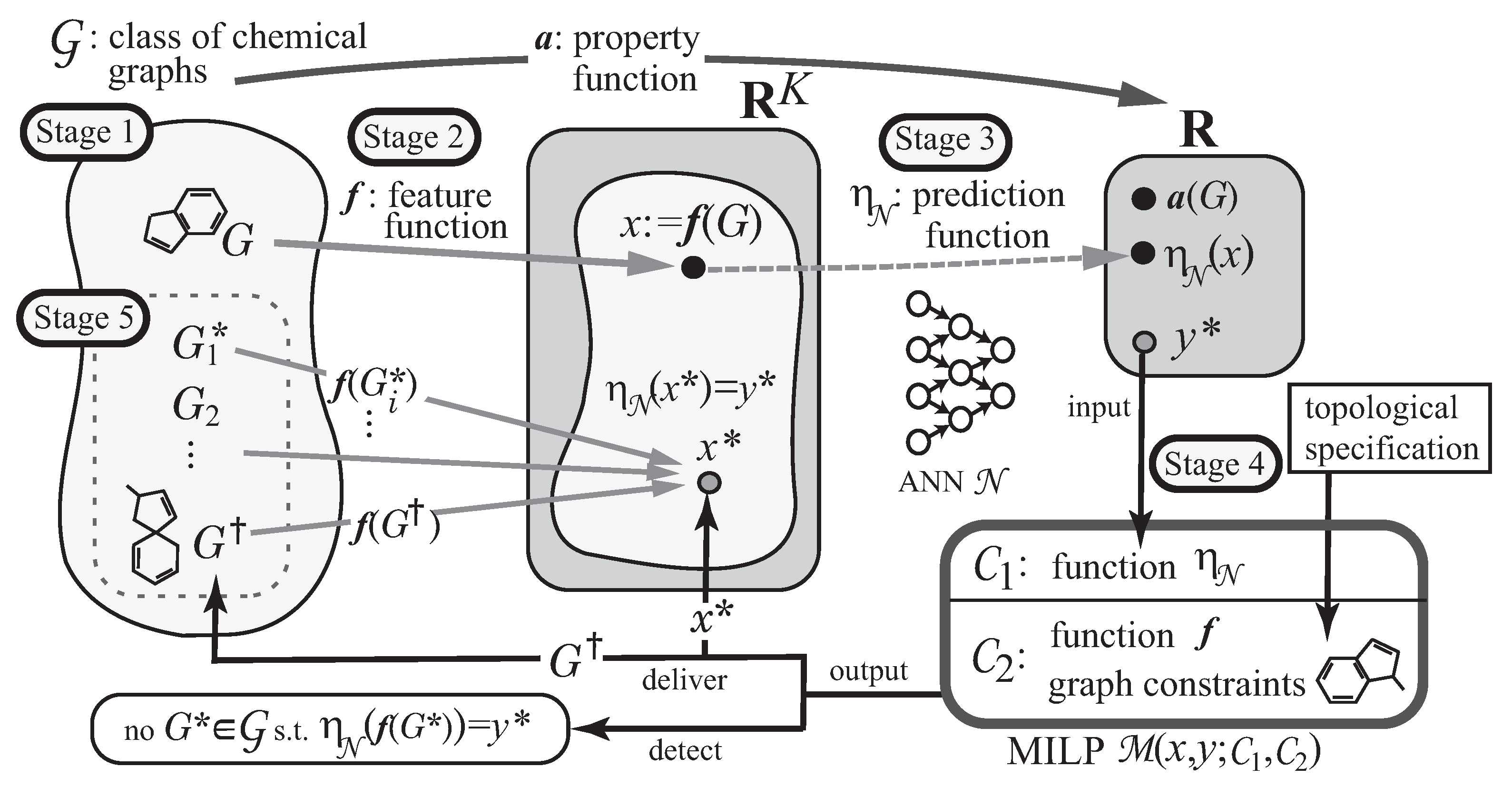
A novel framework for inferring chemical graphs has recently been developed [
22,
23] based on ANNs and mixed integer linear programming (MILP), as illustrated in
Figure 1. It constructs a prediction function in the first phase and infers a chemical graph in the second phase. The first phase of the framework consists of three stages. In Stage 1, we choose a chemical property
and a class
of graphs, where a property function
a is defined so that
is the value of
in
, and collect a data set
of chemical graphs in
such that
is available. In Stage 2, we introduce a feature function
for a positive integer
K. In Stage 3, we construct a prediction function
with an ANN
that, given a vector
, returns a value
so that
serves as a predicted value to
for each
. Given a target chemical value
, the second phase infers chemical graphs
with
in the next two stages. In Stage 4, we formulate an MILP that simulates the construction of
from
G and the computation process in the ANN so that given a target value,
, and solve the MILP to infer a chemical graph
and a feature vector
such that
and
. In Stage 5, we generate other chemical graphs
such that
based on the output chemical graph
.
MILP formulations required in Stage 4 have been designed for chemical compounds with cycle index 0 (i.e., acyclic) [
23,
24], cycle index 1 [
25], and cycle index 2 [
26]. In particular, Azam et al. [
24] introduced a restricted class of acyclic graphs that is characterize by an integer
, called a “branch-parameter” such that the restricted class still covers most of the acyclic chemical compounds in the database.
Recently, Akutsu and Nagamochi [
27] extended the idea to define a restricted class of cyclic graphs, called “
-lean cyclic graphs”, that covers most of the cyclic chemical compounds in the database. Based on this, they also defined a set of rules for specifying several topological substructures of a target chemical graph in a flexible way in Stage 4 before we solve an MILP. The method has been implemented by Zhu et al. [
28], and computational results showed that chemical graphs with around up to 50 non-hydrogen atoms can be inferred. Although the method can infer the class of
-lean cyclic graphs and specify topological structures of the cyclic part, we still need to introduce a new model to deal with an arbitrary graph and to include a prescribed structure in the acyclic part of a target chemical graph.
In this paper, we introduce a new model, called a
two-layered model, for representing the feature of a chemical graph in order to deal with an arbitrary graph in the framework. In the two-layered model, a chemical graph
G with a parameter
is regarded as two parts: the exterior and the interior. The exterior consists of maximal acyclic induced subgraphs with height at most
and the interior is the connected subgraph obtained by ignoring the exterior. We define a feature vector
of a chemical graph
G to be the frequency of adjacent atom pairs in the interior and the frequency of chemical acyclic graphs in the exterior.
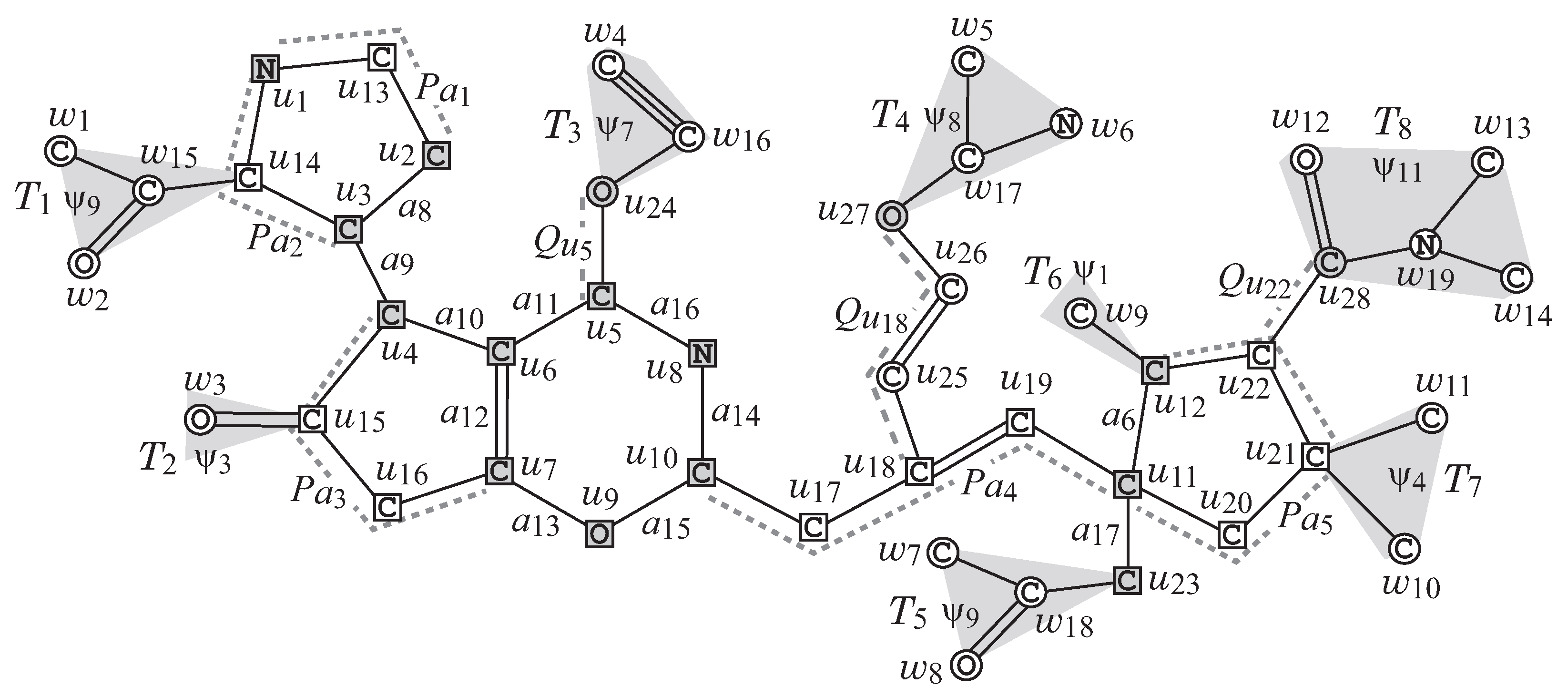
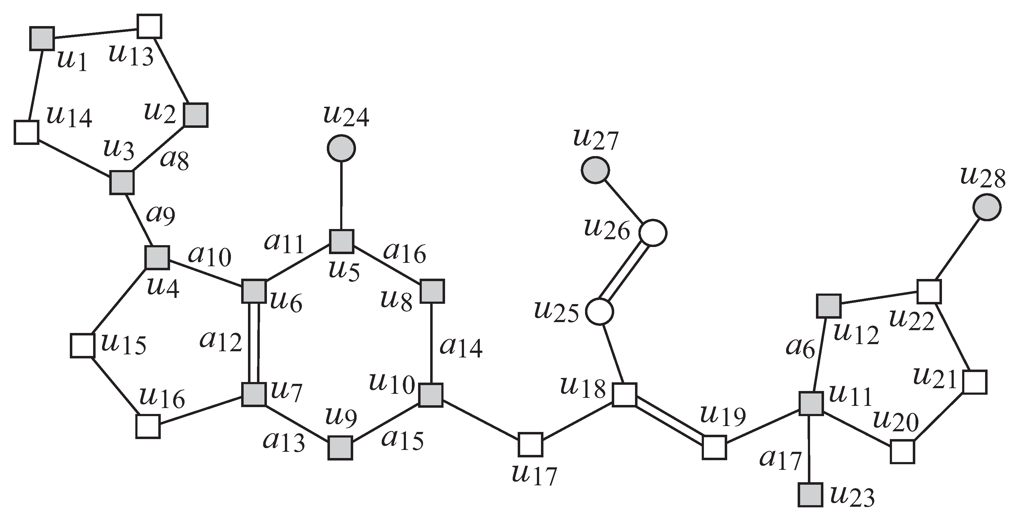
Figure 2 illustrates an example of a chemical graph
G. For a branch-parameter
, the interior of the chemical graph
G in
Figure 2 is obtained by removing the set of vertices with degree 1
times, i.e., first remove the set
of vertices of degree 1 in
G, and then remove the set
of vertices of degree 1 in
, where the removed vertices become the exterior-vertices of
G and there are eight rooted trees
in the exterior of
G.
We also introduce a new set of rules for specifying topological substructures of a target chemical graph
G to be inferred so that a prescribed structure can be included in both of the acyclic and cyclic parts of
G. The set of rules contains (i) a
seed graph as an abstract form of a target chemical graph
G; (ii) a set
of chemical rooted trees as candidates for trees in the exterior of
G; and (iii) lower and upper bounds on the number of components in a target chemical graph such as chemical elements, double/triple bounds and the interior-vertices in
G.
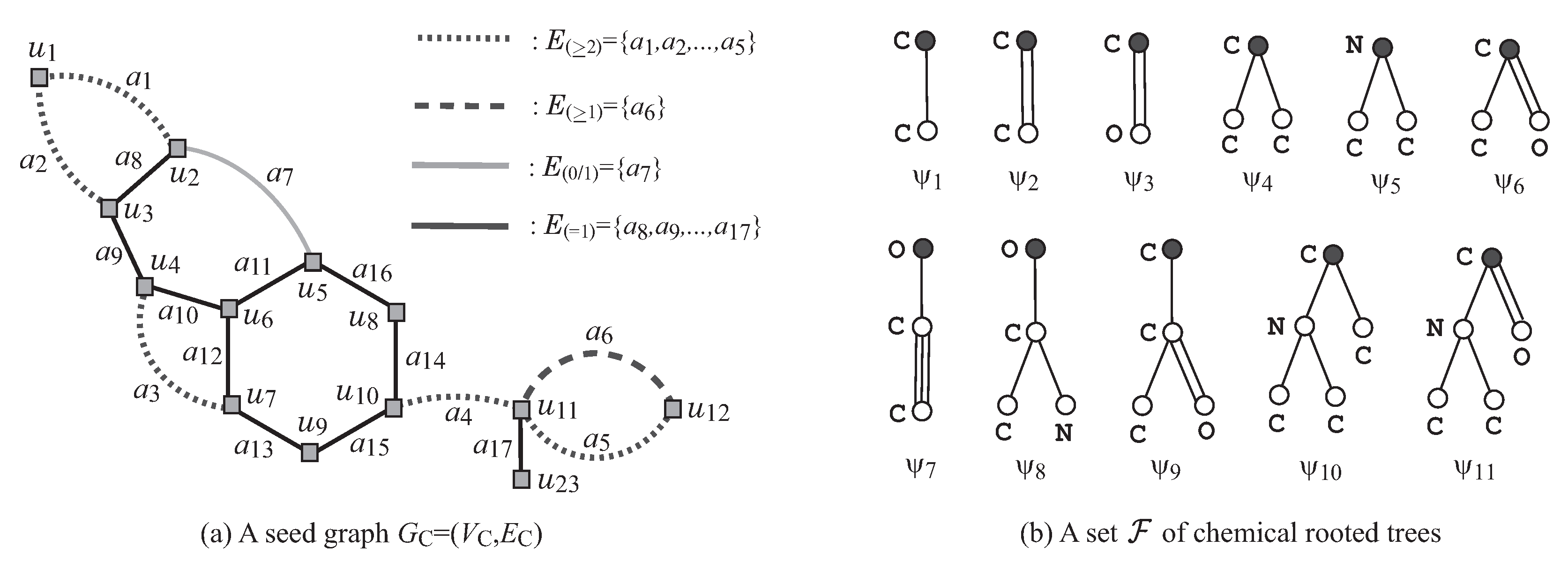
Figure 3a,b illustrates examples of a seed graph
and a set
of chemical rooted trees, respectively. Given a seed graph
, the interior of a target chemical graph
G is constructed from
by replacing some edges
with paths
between the end-vertices
u and
v, and by attaching new paths
to some vertices
v. For example, the chemical graph
G in
Figure 2 is constructed from the seed graph
in
Figure 3a as follows. First replace five edges
and
in
with new paths
,
,
,
and
, respectively, to obtain the subgraph
of
G that consists of vertices depicted with squares. Next, attach to this graph
three new paths,
,
, and
, to obtain the interior of
G in
Figure 2. Finally, the chemical graph
G in
Figure 2 is obtained by attaching eight trees
selected from the set
and assigning chemical elements and bond-multiplicities in the interior. The frequency of chemical elements and the graph size are controlled with lower and upper bounds on the components in a target chemical graph
G. See
Section 2.2 for more details on the specification.
We implemented the two-layered model and the results of computational experiments suggest that the proposed method can infer chemical graphs with around up to 50 non-hydrogen atoms.
The paper is organized as follows.
Section 2.1 introduces some notions on graphs, a modeling of chemical compounds, and a choice of descriptors.
Section 2.2 introduces a method of specifying topological substructures of target chemical graphs in Stage 4.
Section 3 reports the results on some computational experiments conducted for chemical properties such as octanol/water partition coefficient, boiling point, melting point, flash point, lipophylicity, and solubility.
Section 4 makes some concluding remarks. An MILP formulation used in Stage 4 and a review of the dynamic programming algorithm for generating isomers in Stage 5 can be found in
Supplementary Materials. The proposed method/system is available at GitHub
https://github.com/ku-dml/mol-infer.
2. Materials and Methods
This section presents mathematical details of our developed method. Readers not interested in mathematical details can skip this section.
2.1. Preliminary
This section introduces some notions and terminology on graphs, a modeling of chemical compounds, and our choice of descriptors.
Let , and denote the sets of reals, integers and non-negative integers, respectively. For two integers a and b, let denote the set of integers i with .
Graphs. Given a graph G, let and denote the sets of vertices and edges, respectively. For a subset (resp., of a graph G, let (resp., ) denote the graph obtained from G by removing the vertices in (resp., the edges in ), where we remove all edges incident to a vertex in in . The rank of a graph G is defined to be the minimum of an edge subset such that contains no cycle. A path with two end-vertices u and v is called a -path. An edge in a connected graph G is called a bridge if the graph obtained from G by removing edge e is not connected, i.e., consists of two connected graphs containing vertex , . For a cyclic graph G, an edge e is called a core-edge if it is in a cycle of G or is a bridge such that each of the connected graphs , of contains a cycle. A vertex incident to a core-edge is called a core-vertex of G.
A vertex designated in a graph G is called a root. In this paper, we designated at most two vertices as roots, and denote by the set of roots of G. We call a graph G rooted (resp., bi-rooted) if (resp., ), where we call Gunrooted if .
For a graph
G, possibly with roots, a
leaf-vertex is defined to be a non-root vertex
with degree 1, call the edge
incident to a leaf vertex
v a
leaf-edge, and denote
and
the sets of leaf-vertices and leaf-edges in
G, respectively. For a graph or a rooted graph
G, we define graphs
obtained from
G by removing the set of leaf-vertices
i times so that
where we call a vertex
a
leaf k-branch and we say that a vertex
has height
height ht(
in
G. The
height ht(
of a rooted tree
T is defined to be the maximum of ht(
of a vertex
. For an integer
, we call a rooted tree
T k-lean if
T has at most one leaf
k-branch. For an unrooted cyclic graph
G, we regard the set of non-core-edges in
G induces a collection
of trees each of which is rooted at a core-vertex, where we call
G k-lean if each of the rooted trees in
is
k-lean. Nearly 97% of cyclic chemical compounds with up to 100 non-hydrogen atoms in PubChem are 2-lean [
24].
Two-layered Model. Let
G be an unrooted graph. For an integer
, which we call a
branch-parameter, a
two-layered model of
G is a partition of
G into an “interior” and an “exterior” in the following way. We call a vertex
(resp., an edge
of
G an
exterior-vertex (resp.,
exterior-edge) if ht(
(resp.,
e is incident to an exterior-vertex) and denote the sets of exterior-vertices and exterior-edges by
and
, respectively and denote
and
, respectively. We call a vertex in
(resp., an edge in
) an
interior-vertex (resp.,
interior-edge). The set
of exterior-edges forms a collection of connected graphs each of which is regarded as a rooted tree
T rooted at the vertex
with the maximum ht(
, where we call
T a
ρ-fringe-tree (or a fringe-tree). Let
denote the set of fringe-trees in
G. The
interior of
G is defined to be the subgraph
of
G. Note that every core-vertex (resp., core-edge) in
G is an interior-vertex (resp., interior-edge) of
G.
Figure 2 illustrates an example of a graph
G, such that
,
and
for a branch-parameter
.
2.1.1. Modeling of Chemical Compounds
To represent a chemical compound, we assume that each chemical element
has a unique valence
and we use a hydrogen-suppressed model, because hydrogen atoms can be added at the final stage under the assumption. In the hydrogen-suppressed model, a chemical compound
C is represented by a tuple
of a simple, connected undirected graph
H and functions
and
, where
is a set of non-hydrogen chemical elements such as C (carbon), O (oxygen), N (nitrogen), and so on. The set of atoms and the set of bonds in the compound
C are represented by the vertex set
and the edge set
, respectively. The chemical element assigned to a vertex
is represented by
and the bond-multiplicity between two adjacent vertices
is represented by
of the edge
. We say that two tuples
are
isomorphic if they admit an isomorphism
, i.e., a bijection
such that
↔
. When
is rooted at a vertex
,
are
rooted-isomorphic (r-isomorphic) if they admit an isomorphism
such that
. Chemical rooted trees
and
in
Figure 2 are r-isomorphic.
Associated with the two functions and in a tuple , we introduce the following functions: , , , and .
For a notational convenience, we use a function
such that
means the sum of bond-multiplicities of edges incident to a vertex
u, i.e.,
A
chemical graph G is defined to be a tuple
such that the valence condition at each vertex
is satisfied, i.e.,
where we define the
hydro-degree of a vertex
v to be
.
Figure 2 illustrates an example of a chemical graph
.
To represent a feature of an edge such that , and in a chemical graph , we use a tuple , which we call the adjacency-configuration of the edge e. We introduce a total order < over the elements in to distinguish with and notationally. For a tuple , let denote the tuple .
To represent a feature of a vertex with that has d atoms in its neighbor in a chemical graph , we use a pair , which we call the chemical symbol of the vertex v. We treat as a single symbol , and define to be the set of all chemical symbols .
To represent a feature of an edge such that , and in a chemical graph , we use a tuple , which we call the edge-configuration of the edge e. We introduce a total order < over the elements in to distinguish with and notationally. For a tuple , let denote the tuple .
To represent a feature of the exterior of a chemical graph , a -fringe-tree in is called a fringe-configuration in the exterior.
2.1.2. Introducing Descriptors of Feature Vectors
This section introduces descriptors to define our feature vectors. Let be a chemical property for which we will construct a prediction function from a feature vector of a chemical graph to a predicted value for the chemical property of G.
We first choose a set of non-hydrogen chemical elements and then collect a data set of chemical compounds C whose chemical elements belong to , where we regard as a set of chemical graphs that represent the chemical compounds C in . To define the interior/exterior of chemical graphs , we next choose a branch-parameter , where we recommend .
Let (resp., ) denote the set of chemical elements used in the set of interior-vertices (resp., exterior-vertices) over all chemical graphs , and denote the set of edge-configurations used in the set of interior-edges over all chemical graphs . Let denote the set of chemical rooted trees r-isomorphic to a -fringe-tree over all chemical graphs .
We define an integer encoding of a finite set A of elements to be a bijection , where we denote by the set of integers. Introduce an integer coding of each of the sets , , and . Let (resp., ) denote the coded integer of an element (resp., ), denote the coded integer of an element in and denote an element in .
For each chemical element , let and denote the mass and valence of , respectively. In our model, we use integers , .
We define the feature vector of a chemical graph to be a vector that consists of the following non-negative integer descriptors , , where .
: the number of vertices in G.
: the number of interior-vertices in G.
: the average of mass over all non-hydrogen atoms in G, i.e., .
, : the number of interior-vertices of degree d in G.
, : the number of interior-vertices of interior-degree in the interior of G.
, : the number of vertices in G of hydro-degree .
, , : the number of interior-edges with bond multiplicity m in G, i.e., .
, , : the frequency of chemical element in the set of interior-vertices in G.
, , : the frequency of chemical element in the set of exterior-vertices in G.
, , : the frequency of edge-configuration in the set of interior-edges in G.
, , : the frequency of fringe-configuration in the set of -fringe-trees in G.
2.2. Specifying Target Chemical Graphs
Given a prediction function and a target value , we call a chemical graph such that for the feature vector a target chemical graph. This section presents a set of rules for specifying topological substructure of a target chemical graph in a flexible way in Stage 4.
We first describe how to reduce a chemical graph
into an abstract form based on which our specification rules will be defined. To illustrate the reduction process, we use the chemical graph
in
Figure 2.
- R1
Removal of all -fringe-trees: The interior
of
G is obtained by removing the non-root vertices of each
-fringe-trees
.
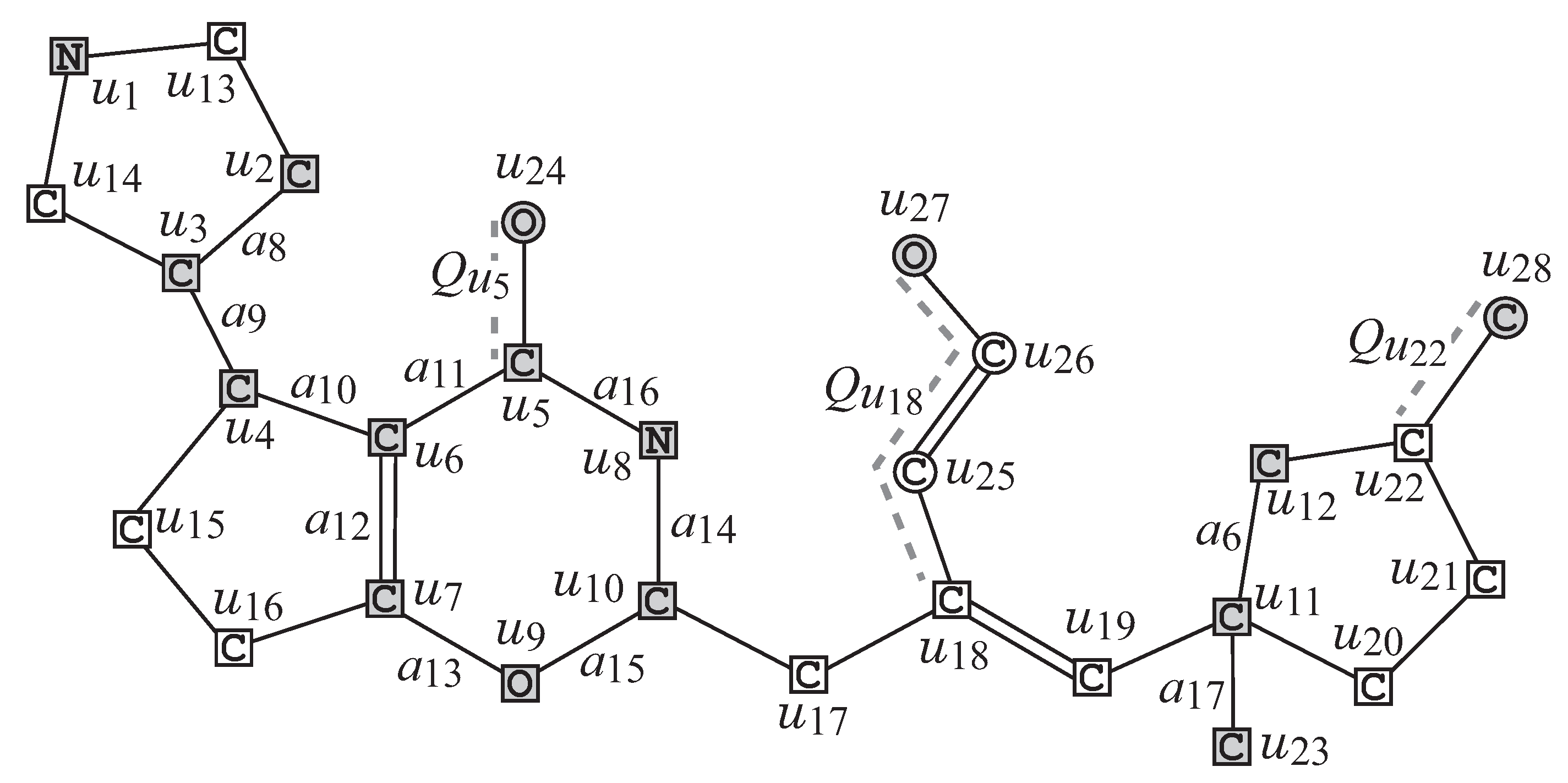
Figure 4 illustrates the interior
of chemical graph
G with
in
Figure 2.
- R2
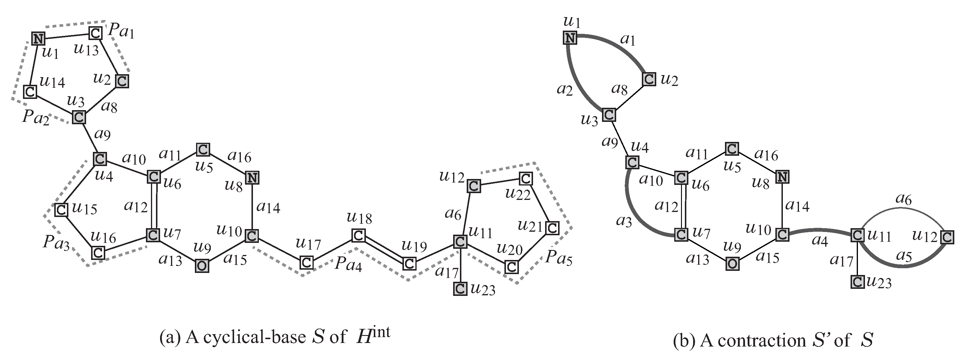
Removal of some leaf paths: We call a
-path
Q in
a
leaf path if vertex
v is a leaf-vertex of
and the degree of each internal vertex of
Q in
is 2, where we regard that
Q is rooted at vertex
u. A connected subgraph
S of the interior
of
G is called a
cyclical-base if
S is obtained from
H by removing the vertices in
for a subset
X of interior-vertices and a set
of leaf
-paths
such that no two paths
and
share a vertex.
Figure 5a illustrates a cyclical-base
of the interior
for a set
of leaf paths in
Figure 4.
- R3
Contraction of some pure paths: A path in
S is called
pure if each internal vertex of the path is of degree 2. Choose a set
of several pure paths in
S so that no two paths share vertices except for their end-vertices. A graph
is called a
contraction of a graph
S (with respect to
) if
is obtained from
S by replacing each pure
-path with a single edge
, where
may contain multiple edges between the same pair of adjacent vertices.
Figure 5b illustrates a contraction
obtained from the chemical graph
S by contracting each
-path
into a new edge
, where
, and
, and
of pure paths in
Figure 5a.
We will define a set of rules so that a chemical graph can be obtained from a graph (called a seed graph in the next section) by applying processes R3 to R1 in a reverse way. We specify topological substructures of a target chemical graph with a tuple called a target specification defined under the set of the following rules.
Seed Graphs
A
seed graph is defined to be a graph (possibly with multiple edges) such that the edge set
consists of four sets
,
,
, and
, where each of them can be empty. A seed graph plays a role of the most abstract form
in R3.
Figure 3a illustrates an example of a seed graph, where
,
,
,
, and
.
A subdivision S of is a graph constructed from a seed graph according to the following rules:
- -
Each edge is replaced with a -path of length at least 2;
- -
Each edge is replaced with a -path of length at least 1 (equivalently e is directly used or replaced with a -path of length at least 2);
- -
Each edge is either used or discarded; and
- -
Each edge is always used directly.
We allow a possible elimination of edges in as an optional rule in constructing a target chemical graph from a seed graph, even though such an operation has not been included in the process R3. A subdivision S plays a role of a cyclical-base in R2. A target chemical graph will contain S as a subgraph of the interior of G.
Interior-Specification
A graph that serves as the interior of a target chemical graph G will be constructed as follows. First, construct a subdivision S of a seed graph by replacing each edge edge with a pure -path . Next, construct a supergraph of S by attaching a leaf path at each vertex or at an internal vertex of each pure -path for some edge , where possibly (i.e., we do not attach any new edges to v). We introduce the following rules for specifying the size of , the length of a pure path , the length of a leaf path , the number of leaf paths , and a bond-multiplicity of each interior-edge, where we call the set of prescribed constants an interior-specification :
- -
Lower and upper bounds on the number of interior-vertices of a target chemical graph G.
- -
For each edge ,
a lower bound and an upper bound on the length of a pure -path . (For a notational convenience, set , , and , , . )
a lower bound and an upper bound on the number of leaf paths attached to at internal vertices v of a pure -path .
a lower bound and an upper bound on the maximum length of a leaf path attached at an internal vertex of a pure -path .
- -
For each vertex ,
a lower bound and an upper bound on the number of leaf paths attached to v, where .
a lower bound and an upper bound on the length of a leaf path attached to v.
- -
For each edge , a lower bound and an upper bound on the number of edges with bond-multiplicity in -path , where we regard , as single edge e.
We call a graph that satisfies an interior-specification a -extension of , where the bond-multiplicity of each edge has been determined.
Table 1 shows an example of an interior-specification
to the seed graph
in
Figure 3.
Figure 6 illustrates an example of an
-extension
of seed graph
in
Figure 3 under the interior-specification
in
Table 1.
Chemical-Specification
Let be a graph that serves as the interior of a target chemical graph G, where the bond-multiplicity of each edge in has be determined. Finally, we introduce a set of rules for constructing a target chemical graph G from by choosing a chemical element and assigning a -fringe-tree to each interior-vertex . We introduce the following rules for specifying the size of G, a set of chemical rooted trees that are allowed to use as -fringe-trees and lower and upper bounds on the frequency of a chemical element, a chemical symbol, and an edge-configuration, where we call the set of prescribed constants a chemical specification :
- -
Lower and upper bounds on the number of vertices in G, where .
- -
Subsets and of chemical rooted trees with height at most , where we require that every -fringe-tree rooted at a vertex (resp., at an internal vertex v not in ) in G belongs to (resp., ). Let and denote the set of chemical elements assigned to non-root vertices over all chemical rooted trees in .
- -
A subset , where we require that every chemical element assigned to an interior-vertex v in G belongs to . Let and (resp., and ) denote the number of vertices (resp., interior-vertices and exterior-vertices) v such that in G.
- -
A set of chemical symbols and a set of edge-configurations with , where we require that the edge-configuration of an interior-edge e in G belongs to . We do not distinguish and .
- -
Define to be the set of adjacency-configurations such that . Let denote the number of interior-edges e such that in G.
- -
Subsets , , we require that every chemical element assigned to a vertex in the seed graph belongs to .
- -
Lower and upper bound functions and on the number of interior-vertices v such that in G.
- -
Lower and upper bound functions on the number of interior-vertices v such that in G.
- -
Lower and upper bound functions on the number of interior-edges e such that in G.
- -
Lower and upper bound functions on the number of interior-edges e such that in G.
We call a chemical graph G that satisfies a chemical specification a -extension of , and denote by the set of all -extensions of .
Table 2 shows an example of a chemical-specification
to the seed graph
in
Figure 3.
Figure 2 illustrates an example of a
-extension of
obtained from the
-extension
in
Figure 6 under the chemical-specification
in
Table 2.
Our specification of topological substructures is similar to that proposed by Akutsu and Nagamochi [
27], wherein a target chemical graph is restricted to
-lean cyclic graphs and prescribed substructures cannot be specified in the acyclic part. In our new method, a chemical graph with any structure can be handled and substructures in the acyclic part can be fixed.
2.3. Examples of Specification
We here present some cases where a target specification can be chosen based on a set of given chemical graphs with a similar structure so that becomes a subset of . In such a case, every target chemical graph in possesses a common structure over the given set .
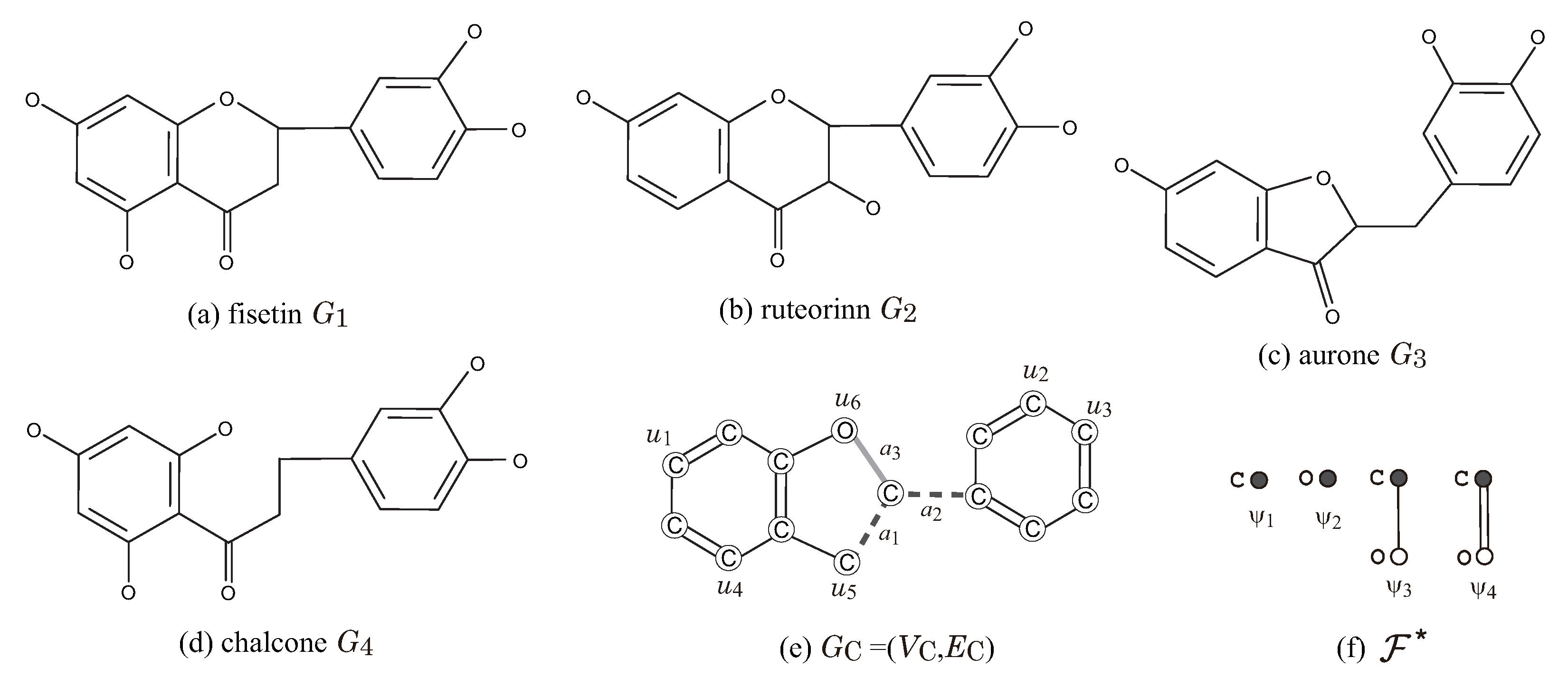
Figure 7 illustrates a set
of four flavonoids and a seed graph
for
so that
for a choice of an interior-specification
and a chemical-specification
. Let
. In the seed graph
, we set
,
, and
and predetermine the chemical element
for each vertex
and the bond-multiplicity
for each edge
as in
Figure 7e, i.e.,
for
and
for
.
Figure 7f illustrates a set
of chemical rooted trees for the 2-fringe-trees in a target chemical graph. For vertices in
, we set
,
,
,
,
, and
. For edges
, we set
and
, where a pure path
may be introduced in a target chemical graph. We see that every given chemical graph
belongs to
by setting the other specification in
and
adequately.
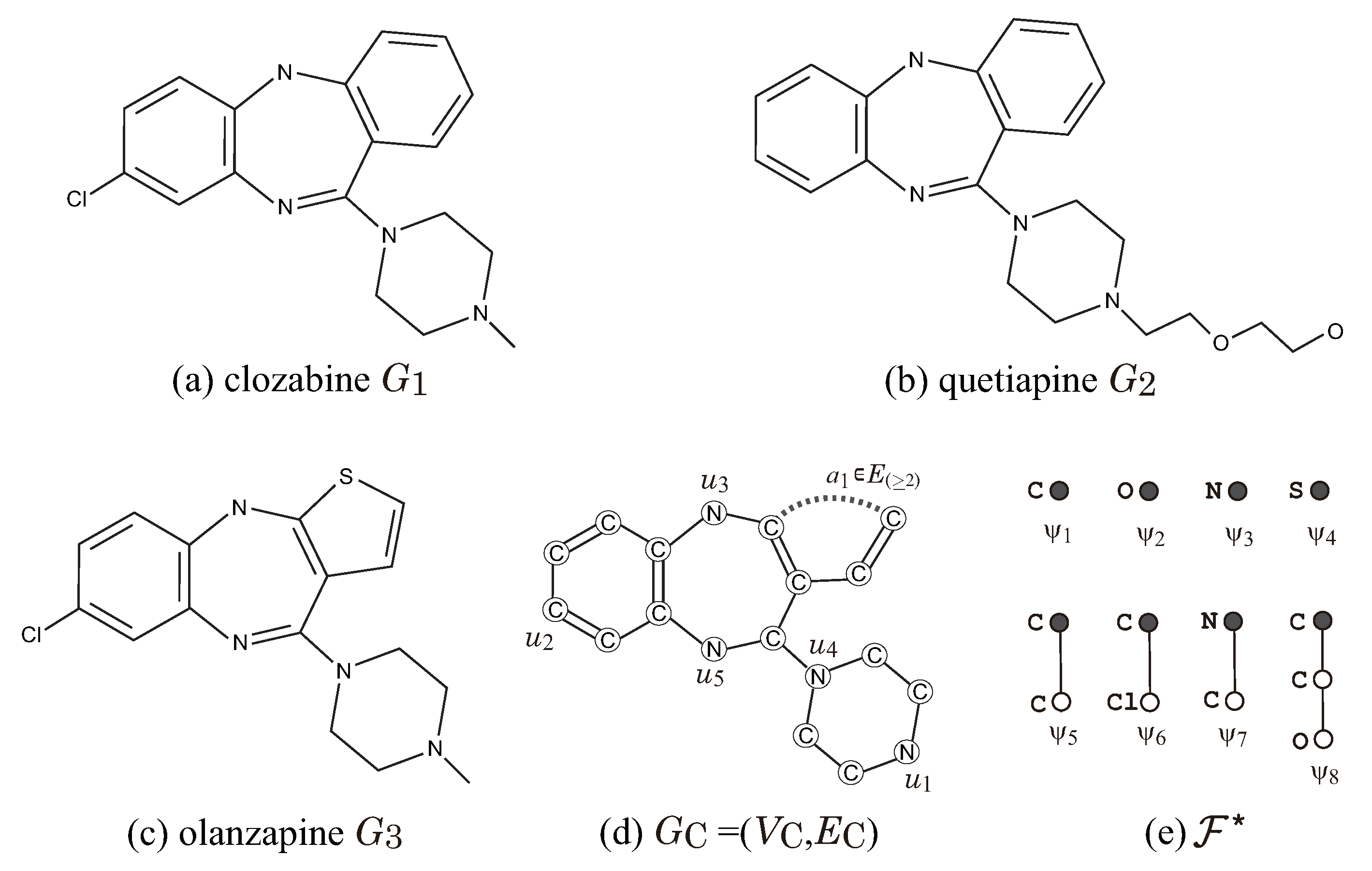
Figure 8 illustrates a set
of three dibenzodiazepine atypical antipsychotics, and a seed graph
for
so that
for a choice of an interior-specification
and a chemical-specification
. Let
. In the seed graph
, we set
and
and predetermine the chemical element
for each vertex
and the bond-multiplicity
for each edge
as in
Figure 8d.
Figure 8e illustrates a set
of chemical rooted trees for the 2-fringe-trees in a target chemical graph. For vertices in
, we set
,
,
,
,
,
, and
, where a leaf path
may be introduced in a target chemical graph. For edge
, we set
and
. We see that every given chemical graph
belongs to
by setting the other specification in
and
adequately.
3. Results
We implemented our method of Stages 1 to 5 for inferring chemical graphs under a given target specification and conducted experiments to evaluate the computational efficiency. We executed the experiments on a PC with Processor: 3.0 GHz Core i7-9700 (3.0 GHz) Memory: 16 GB RAM DDR4. We used ChemDoodle version 10.2.0 for constructing 2D drawings of chemical graphs.
To conduct experiments for Stages 1 to 5, we selected six chemical properties
: octanol/water partition coefficient (K
OW), boiling point (B
P), melting point (M
P), flash point (closed cup) (F
P), lipophylicity (L
P), solubility (S
L) provided by HSDB from PubChem [
29] for K
OW, B
P, M
P, and F
P, figshare [
30] for L
P and MoleculeNet [
31] for S
L.
Results on Phase 1.
We implemented Stages 1, 2, and 3 in Phase 1 as follows.
Stage 1. We set a graph class to be the set of all chemical graphs with any graph structure, and set a branch-parameter to be 2. For each property KOW, BP, MP, FP, LP, SL}, we first select a set of chemical elements and then collect a data set on chemical graphs over the set of chemical elements. To construct the data set , we eliminated chemical compounds that have at most three carbon atoms or contain a charged element such as or an element whose valence is different from our setting of valence function .
Table 3 shows the size and range of data sets that we prepared for each chemical property in Stage 1, where we denote the following:
: the set of selected chemical elements (hydrogen atoms are added at the final stage);
: the size of data set over for property ;
: the number of different edge-configurations of interior-edges over the compounds in ;
: the number of non-isomorphic chemical rooted trees in the set of all 2-fringe-trees in the compounds in ;
: the minimum and maximum values of over the compounds G in ; and
: the minimum and maximum values of in over compounds G in .
Stage 2. We used the new feature function that consists of the descriptors such as fringe-configuration defined in
Section 2.1 and let
denote the feature function.
Stage 3. Let
be a prediction function to a property function
with a feature function
for a data set
D of chemical graphs. We define the coefficient of determination
of a prediction function
over a data set
D to be
To conduct an experiment in Stage 3, we first constructed ten architectures , with one or two hidden layers. For each pair of a property KOW, BP, MP, FP, LP, SL}, and an architecture , , we constructed five prediction functions in order to evaluate the performance with cross-validation as follows. Partition data set into five subsets , randomly and for each set construct an ANN and its prediction function using the feature function . We used scikit-learn version 0.23.2 with Python 3.8.5, MLPRegressor and ReLU activation function to construct each ANN . We evaluated the resulting prediction function with the coefficient of determination for the test set . For each property , let t- denote the average of over all in the cross-validation to an architecture .
Table 4 shows the results on Stages 2 and 3, where we denote the following.
- -
: the set of selected chemical elements (hydrogen atoms are added at the final stage);
- -
L-time: the average time (s) to construct an ANN over all ANNs;
- -
t- (best): the best value of t- over all architectures , ;
- -
t-: the maximum of over all ; and
- -
Arch.: The architecture , that attains t-. An architecture (resp., ) consists of an input layer with K nodes, a hidden layer with p nodes (resp., two hidden layers with and nodes, respectively), and an output layer with a single node, where K is equal to the number of descriptors in the feature vector.
From
Table 4, we see that the execution of Stage 3 was considerably successful, where most of t-
are around 0.85 to 0.95 for all six chemical properties.
An Additional Experiment in Stage 3. We conducted an additional experiment to compare our new feature function
with the feature function
based edge-configuration in the previous method [
27] designed with the same framework. Note that the previous feature vector
can be defined only for a cyclic graph
G, whereas our feature vector
is defined for an arbitrary graph
G. For each property
K
OW, B
P, M
P, F
P, L
P, S
L}, we set a set
of chemical elements to be
and then collect a data set
of chemical cyclic graphs from the data set
of all chemical graphs over the set
of chemical elements in the previous experiment. For each of the feature functions
and
, we constructed five prediction functions with the same set of ten architectures
,
and the data set
of chemical cyclic graphs in the same manner of the previous experiment.
Table 5 shows the results of this experiment, where the table also includes the result of prediction functions by
in the set
of all chemical graphs. In the table, we denote the following:
- -
, : the size of data set of cyclic graphs (resp., of all chemical graphs) for property ;
- -
t- (ave.): the average of over all for and ; and
- -
t- (best): the average of over all .
From
Table 5, we see that the score of R
of the prediction function by
in chemical cyclic graphs (resp., in all chemical graphs) is improved from that by
for properties M
P and F
P (resp., B
P, M
P, and F
P). Recall that our new feature function
can be defined for arbitrary graphs and we can select a larger data set than that by
in a learning stage. This advantage is observed in the experiment. We guess that the better prediction function for B
P (resp., F
P) is obtained by using
because the size of data set becomes considerably larger from
to
(resp., from
to
).
Results on Phase 2.
We prepared the following instances (a–d) for conducting experiments of Stages 4 and 5 in Phase 2.
- (a)
: The instance used in
Section 2.2 to explain the target specification.
- (b)
, : An instance for inferring chemical graphs with rank at most 2. In the four instances , , the following specifications in are common.
Set , set to be the set of all possible symbols in , and set to be the set of all possible edge-configurations. Set , .
The lower bounds , , , , , , , , , are all set to be 0.
The upper bounds , , , , , , , , , are all set to be an upper bound on .
For each property , let denote the set of 2-fringe-trees in the compounds in , and select a subset with , . For each instance , set , .
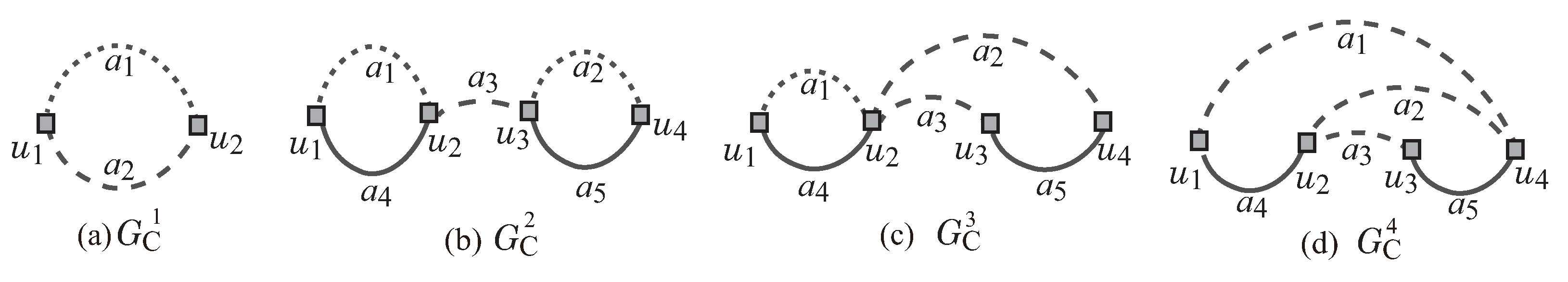
Instance
is given by the rank-1 seed graph
in
Figure 9a and Instances
,
are given by the rank-2 seed graph
,
in
Figure 9b–d.
- (i)
For instance
, select as a seed graph the monocyclic graph
in
Figure 9a, where
,
and
. Set
and
. We include a linear constraint
as part of the side constraint.
- (ii)
For instance
, select as a seed graph the graph
in
Figure 9b, where
,
,
and
. Set
and
. We include a linear constraint
.
- (iii)
For instance
, select as a seed graph the graph
in
Figure 9c, where
,
,
and
. Set
and
. We include linear constraints
and
.
- (iv)
For instance
, select as a seed graph the graph
in
Figure 9d, where
,
and
. Set
and
. We include linear constraints
,
and
.
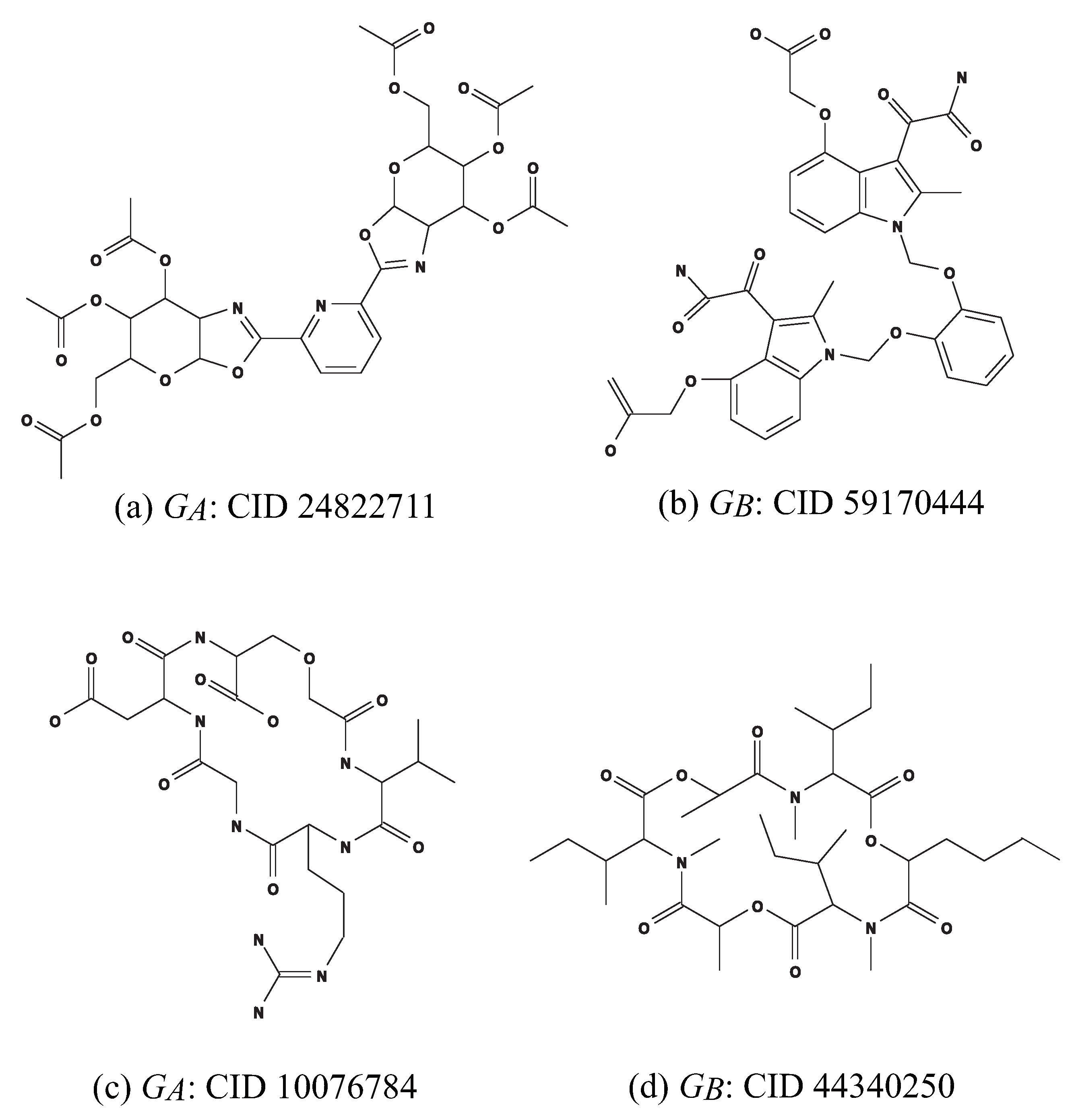
We define instances in (c) and (d) in order to find chemical graphs that have an intermediate structure of given two chemical cyclic graphs and . Let and denote the sets of chemical elements and chemical symbols of the interior-vertices in , denote the sets of edge-configurations of the interior-edges in , and denote the set of 2-fringe-trees in . Analogously define sets , , , and in .
- (c)
: An instance aimed to infer a chemical graph
such that the core of
is equal to the core of
and the frequency of each edge-configuration in the non-core of
is equal to that of
. We use chemical compounds CID 24822711 and CID 59170444 in
Figure 10a,b for
and
, respectively.
Set a seed graph to be the core of .
Set , and set to be the set of all possible chemical symbols in .
Set and , .
Set , ,
and .
Set lower bounds , , , , , , , and to be 0.
Set upper bounds , , , , , , , and to be .
Set to be the number of core-edges in with and to be the number interior-edges in and with edge-configuration .
Let denote the set of chemical rooted trees r-isomorphic p-fringe-trees in .
Set , .
- (d)
: An instance aimed to infer a chemical monocyclic graph
such that the frequency vector of edge-configurations in
is a vector obtained by merging those of
and
. We use chemical monocyclic compounds CID 10076784 and CID 44340250 in
Figure 10c,d for
and
, respectively. Set a seed graph to be the monocyclic seed graph
with
,
and
in
Figure 9a.
Set , and .
Set , ,
and .
Set lower bounds , , , , , , , and to be 0.
Set upper bounds , , , , , , , and to be .
For each edge-configuration , let (resp., ) denote the number of interior-edges with in (resp., ), and set
, ,
and
.
Set , .
In Stage 5, before we formulate an MILP for inferring a target chemical graph
for each instance
I, we reduce the input layer of an ANN
constructed in Stage 3 so that the input layer consists of input nodes that correspond to the descriptors actually used in the specification
of the instance
I, i.e., we remove any input nodes in
that represent the frequency of edge-configurations in
and chemical rooted trees
not contained in the specification
of
I. For example, there are
chemical rooted trees in the set of 2-fringe-trees in the data set
with
K
OW in
Table 3, and an ANN
constructed in Stage 3 contains 109 input nodes that correspond to the descriptors for the fringe-configuration. However, the set of input nodes for the fringe-configuration is reduced to a set of
input nodes when we formulate an MILP for solving instance
, saving the number of integer variables.
Table 6 shows the features of the seven test instances, where we denote the following:
- -
: the set of non-hydrogen chemical elements for inferring a target graph;
- -
: the number of different edge-configurations of interior-edges for inferring a target graph;
- -
: the number of different chemical rooted trees in the set ; and
- -
, : the lower and upper bounds on and for inferring a target graph .
- -
: the minimum and maximum values of
in
over compounds
G in
in
Table 3;
- -
: (resp., ) denotes the minimum (resp., maximum) target value y with such that the MILP instance for the target value becomes feasible (i.e., admits a target chemical graph ). To determine the minimum and minimum target values and , we solved many numbers of MILP instances. Note that the MILP instance may become infeasible for some value y within the range ;
- -
: a target value in for a property ;
- -
#v: the number of variables in the MILP in Stage 4;
- -
#c: the number of constraints in the MILP in Stage 4;
- -
IP-time: the time (sec.) to solve the MILP in Stage 4;
- -
n: the number of non-hydrogen atoms in the chemical graph inferred in Stage 4; and
- -
: the number of interior-vertices in the chemical graph inferred in Stage 4.
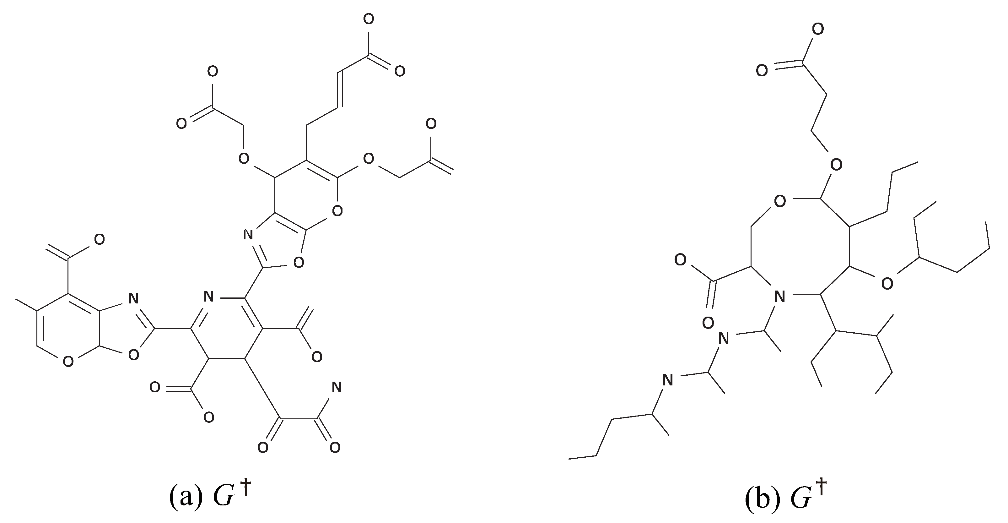
Figure 11a illustrates the chemical graph
inferred from instance
with
of K
OW in
Table 7.
Figure 11b illustrates the chemical graph
inferred from instance
with
of L
P in
Table 11.
The topological specification of instances
,
and
is more restricted than that of the other instances, and thereby the feasible target range
of
,
and
is rather narrower than the original range
for some property
. We see that the running time for solving an MILP instance with
is 8.5 to 122 (s), which is much smaller than the running time of 61 to 12058 (s) to solve a similar set of MILP instances with
in the experimental result for the previous method [
28].
Stage 5. We computed chemical isomers of each target chemical graph inferred in Stage 4. We execute the algorithm for generating chemical isomers of up to 100 when the number of all chemical isomers exceeds 100. The algorithm can evaluate a lower bound on the total number of all chemical isomers without generating all of them.
Table 13 and
Table 14 show the computational results of the experiment, where we denote the following:
- -
DP-time: the running time (s) to execute the dynamic programming algorithm in Stage 5 to compute a lower bound on the number of all chemical isomers of and generate all (or up to 100) chemical isomers ;
- -
G-LB: a lower bound on the number of all chemical isomers of ; and
- -
#G: the number of all (or up to 100) chemical isomers of generated in Stage 5.
From
Table 13 and
Table 14, we observe that the running time for generating up to 100 target chemical graphs in Stage 5 is not considerably larger than that in Stage 4.
4. Discussions and Conclusions
The framework of designing chemical graphs using ANNs and MILP has been proposed [
23] as a basis of a total system of the QSAR and the inverse of QSAR, where the inverse of a prediction function produced by an ANN is solved by an MILP. The merit of the framework is that the inverse problem can be treated exactly as a mathematical problem, and an MILP instance with a moderate size can be efficiently solved with a fast MILP solver. On the other hand, the main technical concern in applying the framework is in defining a feature vector of a chemical graph in terms of graph theoretical descriptors so that the computation of a feature vector can be simulated with a set of linear constraints in an MILP. So far, the framework has been applied to the design of new methods of inferring several restricted classes of chemical graphs such as the graphs with rank at most 2 and the
-lean cyclic graphs [
26,
28].
Herein, we examine some technical issues in the previous method before we observe some new features of our method in this paper.
In the feature vector of the previous models [
26,
28], the structure of subgraphs used as descriptors is only a pair of adjacent vertices, called adjacency-configuration or edge-configuration, which is significantly limited from a variety of subgraphs used in a more sophisticated construction of a feature vector such as the fingerprint. However, including the occurrence of a certain subgraph with only a few vertices as part of a feature vector may require realizing a mechanism of the subgraph isomorphism in an MILP that simulates the computation of such an occurrence and can easily make the resulting MILP very complicated and hard to solve. Furthermore, the feature vector can be defined only for cyclic graphs and we need to eliminate any acyclic graphs from the original data set before we construct a prediction function. This may reduce a data set to an unnecessarily small size or reduce the chances of capturing important information on QSAR over all types of graphs.
A branch-parameter
was originally introduced as a new measure to the “agglomeration degree” of trees [
24] and then used to define restricted classes of acyclic and cyclic graphs [
24,
27]. In fact, such a restriction on the structure of target chemical graphs was rather necessary to reduce the size of an MILP formulation that simulates a selection process of a target chemical graph from a supergraph (called a scheme graph), where the number of variables and constraints required to infer a chemical graph with
non-hydrogen atoms is
when some other parameters such as
are regarded as constants.
Although nearly 97% of cyclic chemical compounds with up to 100 non-hydrogen atoms in PubChem are 2-lean [
24], the way of specifying the topological structure of a target chemical graph in the previous method [
26,
28] was based on the core and the non-core of a chemical graph, and we could not include a fixed substructure in the non-core of a target chemical graph.
Compared with the previous models, the two-layered model proposed in this paper is rather simple, where a chemical graph is regarded as a combination of the interior and the exterior. The new model can deal with chemical compounds with any graph structure and include a prescribed structure in both of the acyclic and cyclic parts of a target chemical graph as long as the requirement on target chemical graphs is described under the set of specification rules introduced in this paper. This considerably improves the availability of the framework in a practical application.
The feature vector of our two-layered model can be defined for arbitrary graphs. In the new feature vector, the exterior of a chemical graph is encoded into fringe-configurations, i.e., the occurrence of each chemical rooted tree with height at most , where we may regard that the set of such a chemical rooted trees plays a similar role of some types of functional groups. In our method, we include as part of the descriptors of a feature vector the occurrence of each of such chemical rooted trees and the descriptors of our feature vector on the exterior of a chemical graph may have an analogous effect with the fingerprint.
Our specification of target chemical graphs can specify a candidate set of chemical rooted trees that are allowed to be used as chemical rooted trees in the exterior of a target chemical graph. This allows us to control the chemical property of target chemical graphs in a more meaningful way since chemical properties of some rooted trees in are known as functional groups and some kinds of rooted trees can be prohibited in a target chemical graph, if necessary, just by excluding from the candidate set . Although the number of different kinds of such chemical trees in a data set from PubChem is approximately up to 300 for in many cases and the number of input nodes in an ANN becomes over , we derived an MILP formulation for inferring a chemical graph with with non-hydrogen atoms and a candidate set of chemical rooted trees by using variables and constraints when the number of interior-vertices is constant, where can be quite small compared with .
We have implemented the proposed method for inferring chemical compounds with a prescribed topological substructure setting . The results of computational experiments using some chemical properties such as octanol/water partition coefficient, boiling point, melting point, flash point, lipophylicity, and solubility suggest that the proposed system can infer chemical graphs with 50 non-hydrogen atoms.
For a larger branch-parameter, say , we obtain a more variety of chemical rooted trees which provides new descriptors in a feature vector and new candidates for fringe-trees in the exterior in a target chemical graph, whereas the number of different chemical rooted trees in may increase rapidly.
It is left as a future work to use other learning methods such as decision tree, random forest, graph convolution, and an ensemble method in Stages 3 and 4 in the framework.


 ,
, 


