
Direct Measurement of the Affinity between tBid and Bax in a Mitochondria-Like Membrane

 , and
, and 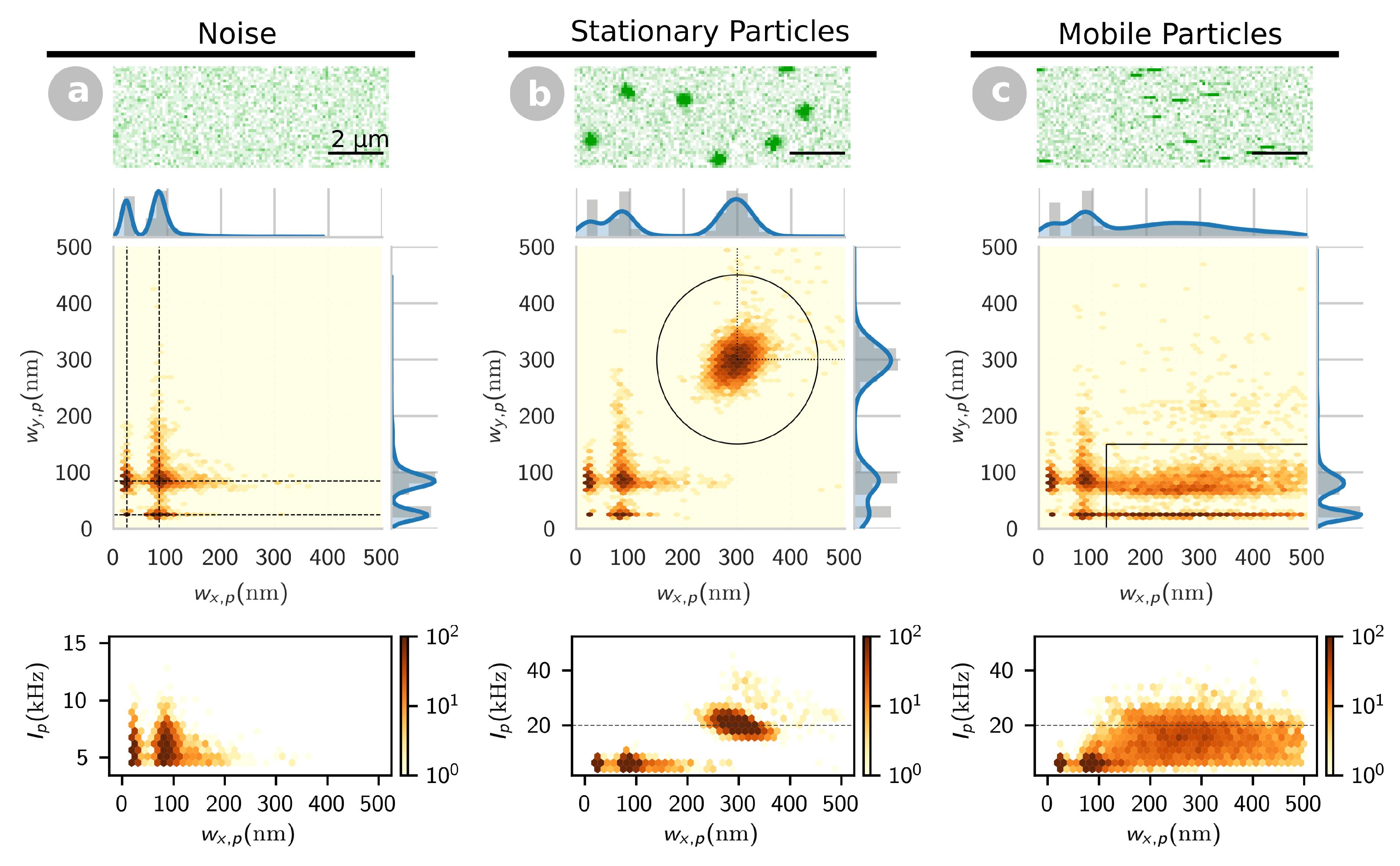
Abstract
:1. Introduction
2. Results
2.1. Different Membrane Conformations Are Detected for tBid and Bax Based on Their Mobility
2.1.1. Signature of Stationary and Mobile Particles in Confocal Images
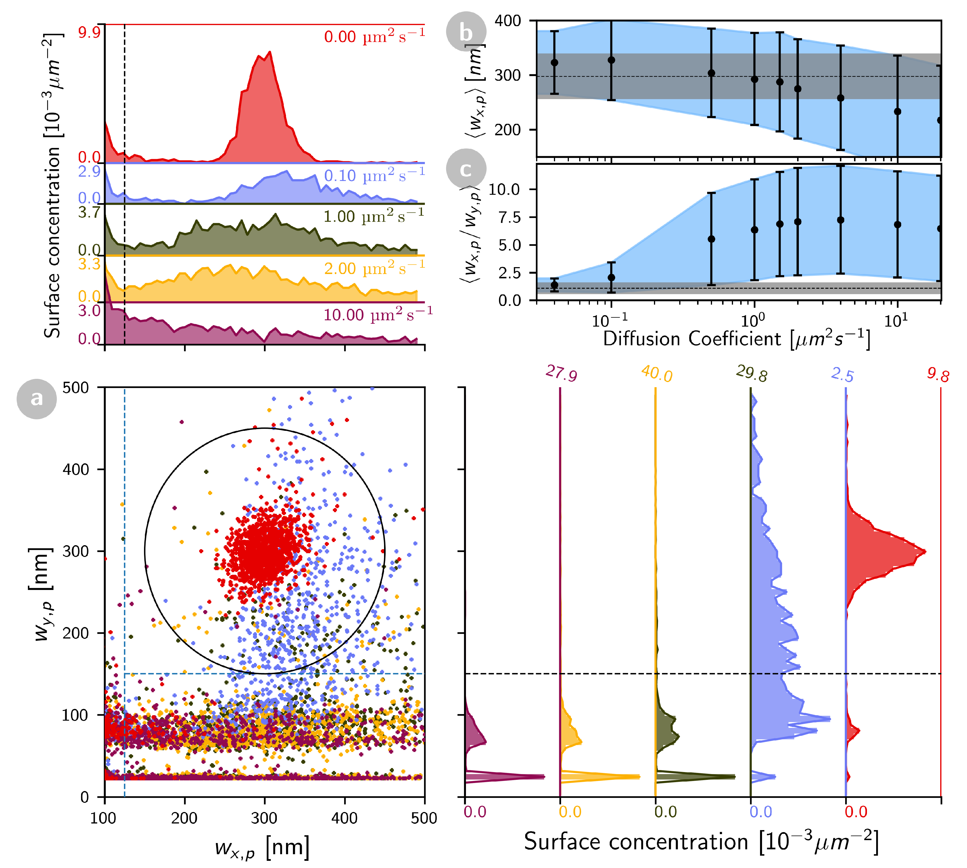
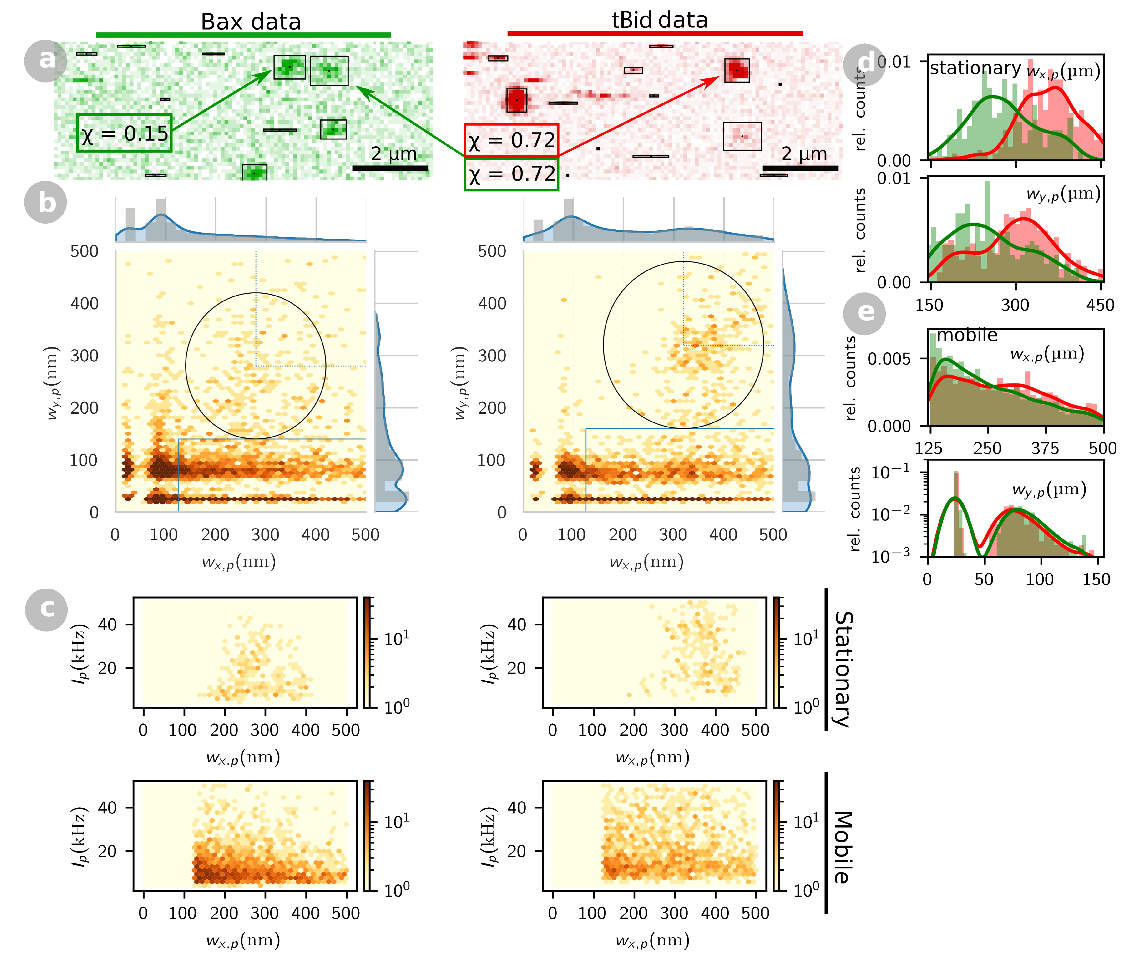
2.1.2. tBid and Bax Mobility in the Mitochondria-Like SLB
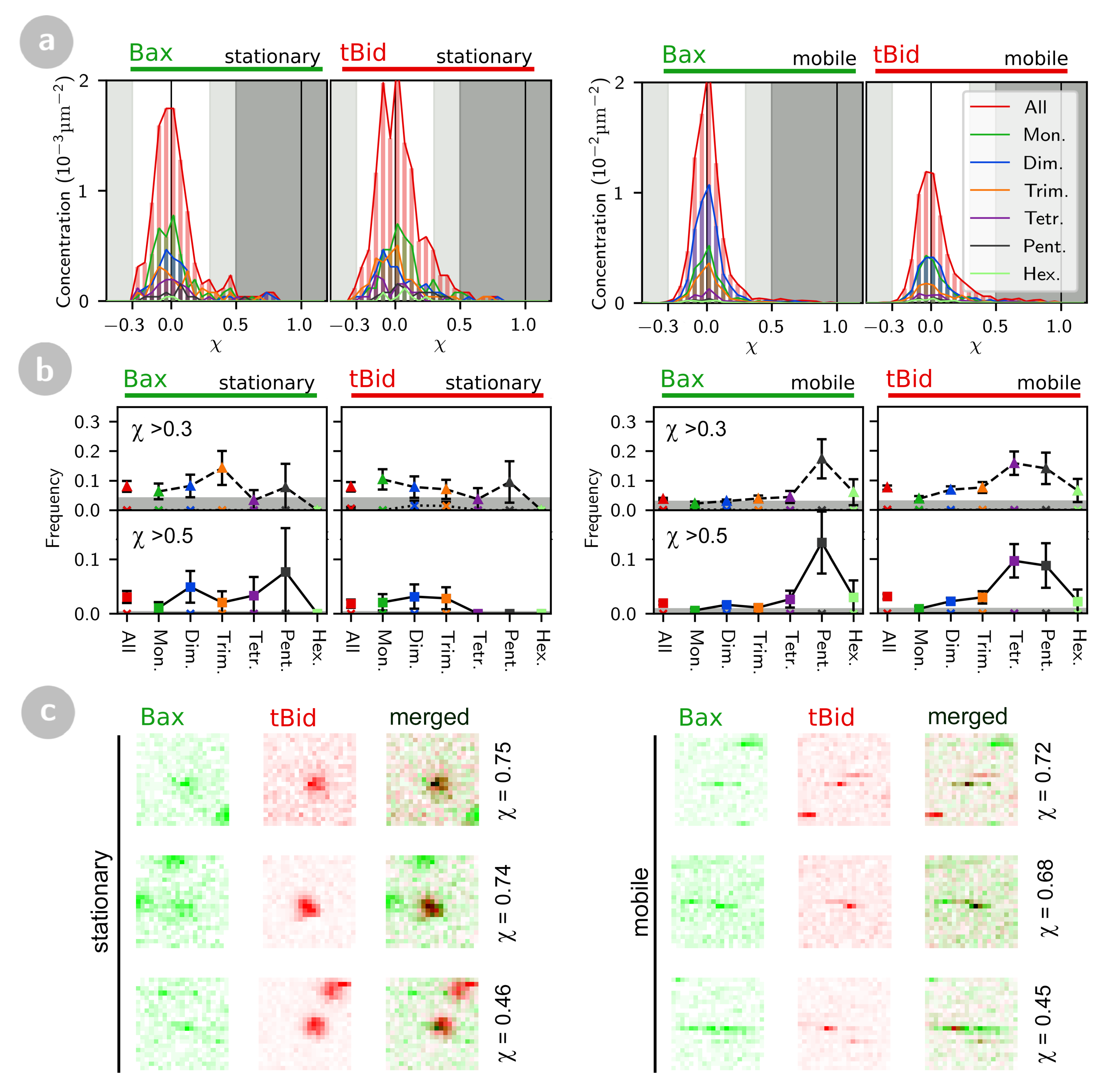
2.2. tBid and Bax form Oligomers at the Membrane
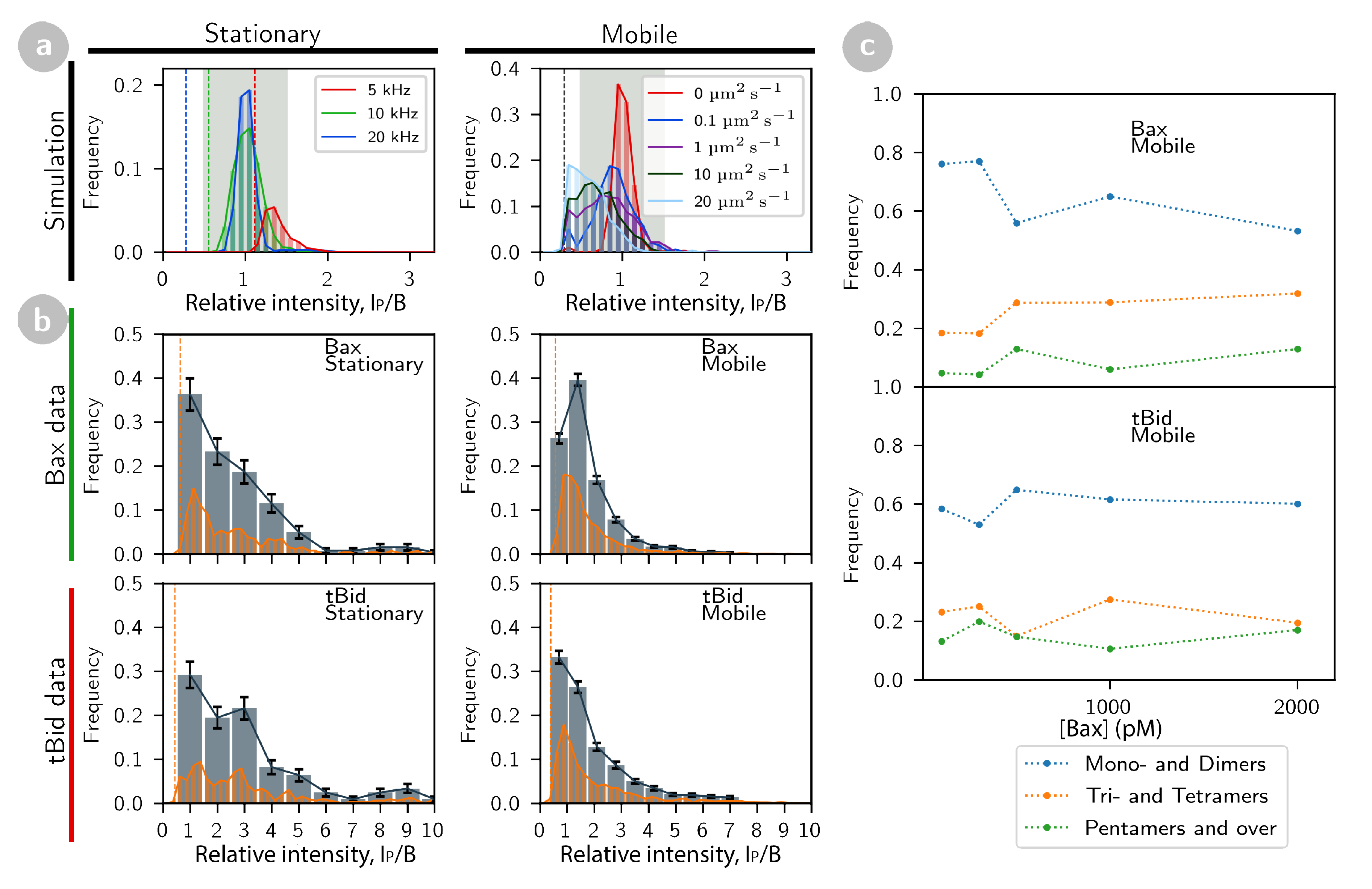
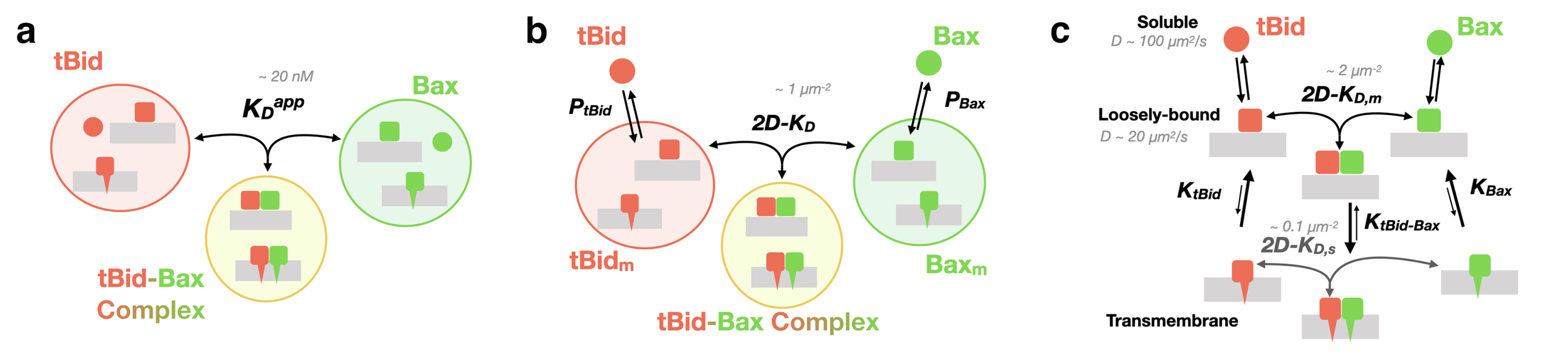
2.3. Quantification of the Interaction between tBid and Bax
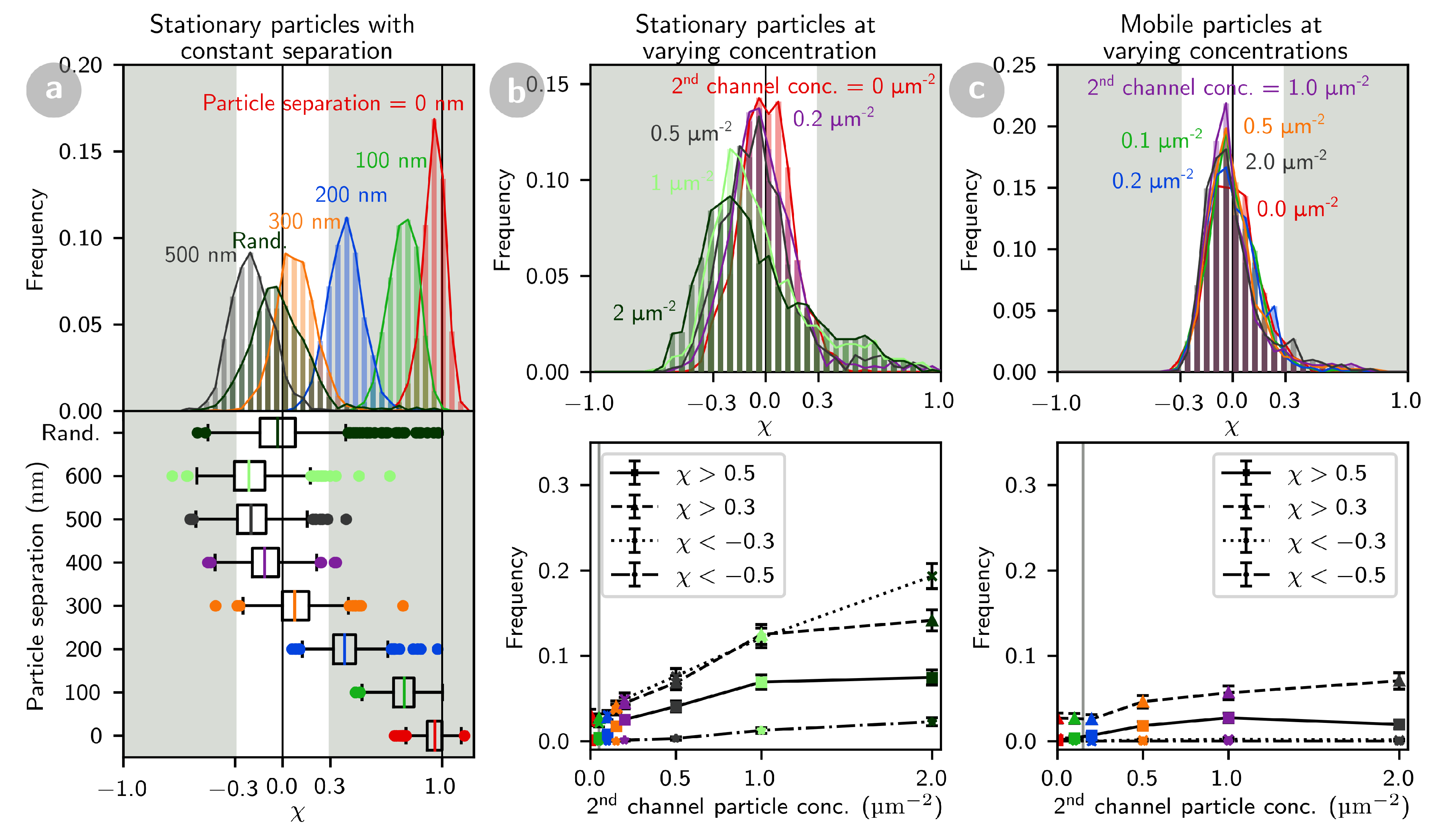
2.3.1. The Particle Cross-Correlation Coefficient Decreases with the Distance between Particles
2.3.2. Co-Localization of tBid and Bax
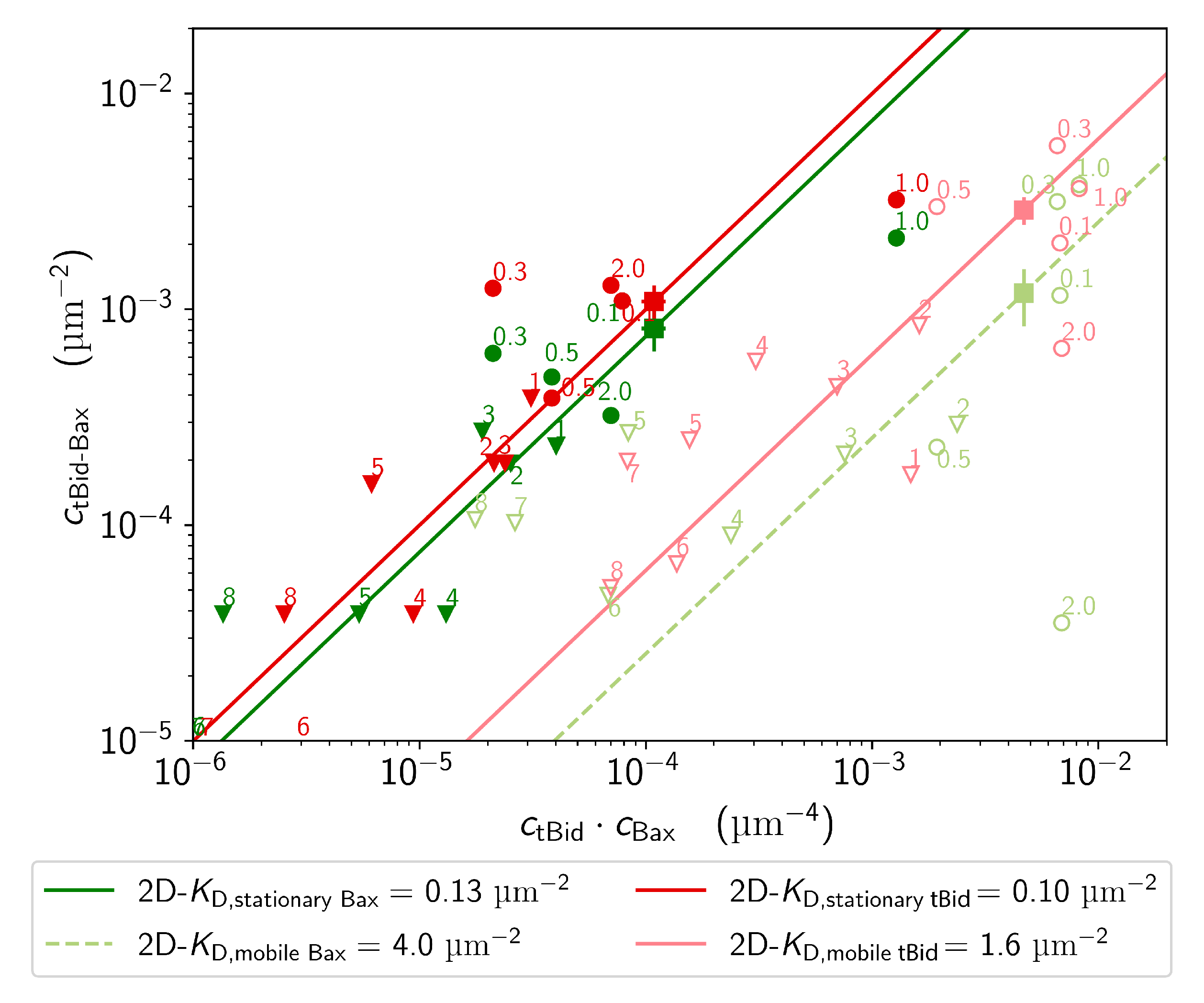
2.3.3. Dissociation Constant of tBid-Bax Complexes
3. Discussion
4. Materials and Methods
4.1. Protein Purification and Labelling
4.1.1. tBid
4.1.2. Bax
4.1.3. Purified Protein Activity
4.2. Mitochondria-Like Supported Lipid Bilayers
4.3. Confocal Imaging
4.4. Simulations
4.5. Image Analysis
4.5.1. Single Particle Detection
4.5.2. Single Particle Cross-Correlation Coefficient
4.5.3. Dissociation Constant
Supplementary Materials
Author Contributions
Funding
Institutional Review Board Statement
Informed Consent Statement
Acknowledgments
Conflicts of Interest
References
- Kalkavan, H.; Green, D.R. MOMP, cell suicide as a BCL-2 family business. Cell Death Differ. 2018, 25, 46. [Google Scholar] [CrossRef]
- Kale, J.; Osterlund, E.J.; Andrews, D.W. BCL-2 family proteins: Changing partners in the dance towards death. Cell Death Differ. 2018, 25, 65. [Google Scholar] [CrossRef] [Green Version]
- Kelekar, A.; Thompson, C.B. Bcl-2-family proteins: The role of the BH3 domain in apoptosis. Trends Cell Biol. 1998, 8, 324–330. [Google Scholar] [CrossRef]
- Moldoveanu, T.; Follis, A.V.; Kriwacki, R.W.; Green, D.R. Many players in BCL-2 family affairs. Trends Biochem. Sci. 2014, 39, 101–111. [Google Scholar] [CrossRef] [Green Version]
- Westphal, D.; Kluck, R.; Dewson, G. Building blocks of the apoptotic pore: How Bax and Bak are activated and oligomerize during apoptosis. Cell Death Differ. 2014, 21, 196–205. [Google Scholar] [CrossRef] [PubMed] [Green Version]
- Eskes, R.; Desagher, S.; Antonsson, B.; Martinou, J.C. Bid induces the oligomerization and insertion of Bax into the outer mitochondrial membrane. Mol. Cell. Biol. 2000, 20, 929–935. [Google Scholar] [CrossRef] [PubMed] [Green Version]
- Kuwana, T.; Mackey, M.R.; Perkins, G.; Ellisman, M.H.; Latterich, M.; Schneiter, R.; Green, D.R.; Newmeyer, D.D. Bid, Bax, and lipids cooperate to form supramolecular openings in the outer mitochondrial membrane. Cell 2002, 111, 331–342. [Google Scholar] [CrossRef] [Green Version]
- Putcha, G.V.; Le, S.; Frank, S.; Besirli, C.G.; Clark, K.; Chu, B.; Alix, S.; Youle, R.J.; LaMarche, A.; Maroney, A.C.; et al. JNK-mediated BIM phosphorylation potentiates BAX-dependent apoptosis. Neuron 2003, 38, 899–914. [Google Scholar] [CrossRef] [Green Version]
- Walensky, L.D.; Pitter, K.; Morash, J.; Oh, K.J.; Barbuto, S.; Fisher, J.; Smith, E.; Verdine, G.L.; Korsmeyer, S.J. A stapled BID BH3 helix directly binds and activates BAX. Mol. Cell 2006, 24, 199–210. [Google Scholar] [CrossRef]
- Lovell, J.F.; Billen, L.P.; Bindner, S.; Shamas-Din, A.; Fradin, C.; Leber, B.; Andrews, D.W. Membrane binding by tBid initiates an ordered series of events culminating in membrane permeabilization by Bax. Cell 2008, 135, 1074–1084. [Google Scholar] [CrossRef] [Green Version]
- Chi, X.; Pemberton, J.; Nguyen, D.; Osterlund, E.J.; Liu, Q.; Brahmbhatt, H.; Zhang, Z.; Lin, J.; Leber, B.; Andrews, D.W. The carboxyl-terminal sequence of bim enables bax activation and killing of unprimed cells. eLife 2020, 9, e44525. [Google Scholar] [CrossRef]
- Singh, R.; Letai, A.; Sarosiek, K. Regulation of apoptosis in health and disease: The balancing act of BCL-2 family proteins. Nat. Rev. Mol. Cell Biol. 2019, 20, 175–193. [Google Scholar] [CrossRef]
- Knight, T.; Luedtke, D.; Edwards, H.; Taub, J.W.; Ge, Y. A delicate balance-The BCL-2 family and its role in apoptosis, oncogenesis, and cancer therapeutics. Biochem. Pharmacol. 2019, 162, 250–260. [Google Scholar] [CrossRef]
- Hafezi, S.; Rahmani, M. Targeting BCL-2 in Cancer: Advances, Challenges, and Perspectives. Cancers 2021, 13, 1292. [Google Scholar] [CrossRef]
- Pogmore, J.P.; Uehling, D.; Andrews, D.W. Pharmacological Targeting of Executioner Proteins: Controlling Life and Death. J. Med. Chem. 2021, 64, 5276–5290. [Google Scholar] [CrossRef] [PubMed]
- Leber, B.; Lin, J.; Andrews, D.W. Embedded together: The life and death consequences of interaction of the Bcl-2 family with membranes. Apoptosis 2007, 12, 897–911. [Google Scholar] [CrossRef] [Green Version]
- Bogner, C.; Leber, B.; Andrews, D.W. Apoptosis: Embedded in membranes. Curr. Opin. Cell Biol. 2010, 22, 845–851. [Google Scholar] [CrossRef] [PubMed]
- Westphal, D.; Dewson, G.; Czabotar, P.E.; Kluck, R.M. Molecular biology of Bax and Bak activation and action. Biochim. Biophys. Acta BBA Mol. Cell Res. 2011, 1813, 521–531. [Google Scholar] [CrossRef] [Green Version]
- Luo, X.; O’Neill, K.L.; Huang, K. The third model of Bax/Bak activation: A Bcl-2 family feud finally resolved? F1000Research 2020, 9. [Google Scholar] [CrossRef] [PubMed]
- Shamas-Din, A.; Bindner, S.; Chi, X.; Leber, B.; Andrews, D.W.; Fradin, C. Distinct lipid effects on tBid and Bim activation of membrane permeabilization by pro-apoptotic Bax. Biochem. J. 2015, 467, 495–505. [Google Scholar] [CrossRef]
- Yang, F.; Qu, W.; Du, M.; Mai, Z.; Wang, B.; Ma, Y.; Wang, X.; Chen, T. Stoichiometry and regulation network of Bcl-2 family complexes quantified by live-cell FRET assay. Cell. Mol. Life Sci. 2020, 77, 2387–2406. [Google Scholar] [CrossRef] [PubMed]
- Edlich, F.; Banerjee, S.; Suzuki, M.; Cleland, M.M.; Arnoult, D.; Wang, C.; Neutzner, A.; Tjandra, N.; Youle, R.J. Bcl-xL retrotranslocates Bax from the mitochondria into the cytosol. Cell 2011, 145, 104–116. [Google Scholar] [CrossRef] [PubMed] [Green Version]
- Todt, F.; Cakir, Z.; Reichenbach, F.; Youle, R.; Edlich, F. The C-terminal helix of Bcl-x L mediates Bax retrotranslocation from the mitochondria. Cell Death Differ. 2013, 20, 333. [Google Scholar] [CrossRef] [PubMed]
- Shamas-Din, A.; Satsoura, D.; Khan, O.; Zhu, W.; Leber, B.; Fradin, C.; Andrews, D. Multiple partners can kiss-and-run: Bax transfers between multiple membranes and permeabilizes those primed by tBid. Cell Death Dis. 2014, 5, e1277. [Google Scholar] [CrossRef] [Green Version]
- García-Sáez, A.J.; Ries, J.; Orzáez, M.; Pérez-Payà, E.; Schwille, P. Membrane promotes tBID interaction with BCL XL. Nat. Struct. Mol. Biol. 2009, 16, 1178. [Google Scholar] [CrossRef] [Green Version]
- Bleicken, S.; Hantusch, A.; Das, K.K.; Frickey, T.; Garcia-Saez, A.J. Quantitative interactome of a membrane Bcl-2 network identifies a hierarchy of complexes for apoptosis regulation. Nat. Commun. 2017, 8, 73. [Google Scholar] [CrossRef]
- Murad, F.; Garcia-Saez, A.J. Quantification of the Interactions Between BCL-2 Proteins by Fluorescence Correlation Spectroscopy. In BCL-2 Family Proteins; Springer: Berlin/Heidelberg, Germany, 2019; pp. 337–350. [Google Scholar]
- Dlugosz, P.J.; Billen, L.P.; Annis, M.G.; Zhu, W.; Zhang, Z.; Lin, J.; Leber, B.; Andrews, D.W. Bcl-2 changes conformation to inhibit Bax oligomerization. EMBO J. 2006, 25, 2287–2296. [Google Scholar] [CrossRef] [PubMed] [Green Version]
- Shivakumar, S.; Kurylowicz, M.; Hirmiz, N.; Manan, Y.; Friaa, O.; Shamas-Din, A.; Masoudian, P.; Leber, B.; Andrews, D.W.; Fradin, C. The proapoptotic protein tBid forms both superficially bound and membrane-inserted oligomers. Biophys. J. 2014, 106, 2085–2095. [Google Scholar] [CrossRef] [Green Version]
- Subburaj, Y.; Cosentino, K.; Axmann, M.; Pedrueza-Villalmanzo, E.; Hermann, E.; Bleicken, S.; Spatz, J.; García-Sáez, A.J. Bax monomers form dimer units in the membrane that further self-assemble into multiple oligomeric species. Nat. Commun. 2015, 6, 8042. [Google Scholar] [CrossRef] [Green Version]
- Kasai, R.S.; Suzuki, K.G.; Prossnitz, E.R.; Koyama-Honda, I.; Nakada, C.; Fujiwara, T.K.; Kusumi, A. Full characterization of GPCR monomer–dimer dynamic equilibrium by single molecule imaging. J. Cell Biol. 2011, 192, 463–480. [Google Scholar] [CrossRef] [Green Version]
- Dupont, A.; Stirnnagel, K.; Lindemann, D.; Lamb, D. Tracking image correlation: Combining single-particle tracking and image correlation. Biophys. J. 2013, 104, 2373–2382. [Google Scholar] [CrossRef] [Green Version]
- Friaa, O.; Fradin, C. Coincidence Measurements in Dual-Color Confocal Microscopy: A Combined Single-Particle and Fluorescence Correlation Approach. Biophys. Rev. Lett. 2014, 9, 249–271. [Google Scholar] [CrossRef]
- Wang, K.; Yin, X.M.; Chao, D.T.; Milliman, C.L.; Korsmeyer, S.J. BID: A novel BH3 domain-only death agonist. Genes Dev. 1996, 10, 2859–2869. [Google Scholar] [CrossRef] [Green Version]
- Shamas-Din, A.; Brahmbhatt, H.; Leber, B.; Andrews, D.W. BH3-only proteins: Orchestrators of apoptosis. Biochim. Biophys. Acta BBA Mol. Cell Res. 2011, 1813, 508–520. [Google Scholar] [CrossRef] [PubMed] [Green Version]
- Chou, J.J.; Li, H.; Salvesen, G.S.; Yuan, J.; Wagner, G. Solution structure of BID, an intracellular amplifier of apoptotic signaling. Cell 1999, 96, 615–624. [Google Scholar] [CrossRef] [Green Version]
- McDonnell, J.M.; Fushman, D.; Milliman, C.L.; Korsmeyer, S.J.; Cowburn, D. Solution structure of the proapoptotic molecule BID: A structural basis for apoptotic agonists and antagonists. Cell 1999, 96, 625–634. [Google Scholar] [CrossRef] [Green Version]
- Hinds, M.; Smits, C.; Fredericks-Short, R.; Risk, J.; Bailey, M.; Huang, D.; Day, C. Bim, Bad and Bmf: Intrinsically unstructured BH3-only proteins that undergo a localized conformational change upon binding to prosurvival Bcl-2 targets. Cell Death Differ. 2007, 14, 128–136. [Google Scholar] [CrossRef] [Green Version]
- Rautureau, G.J.; Day, C.L.; Hinds, M.G. Intrinsically disordered proteins in bcl-2 regulated apoptosis. Int. J. Mol. Sci. 2010, 11, 1808–1824. [Google Scholar] [CrossRef] [Green Version]
- Peng, Z.; Xue, B.; Kurgan, L.; Uversky, V. Resilience of death: Intrinsic disorder in proteins involved in the programmed cell death. Cell Death Differ. 2013, 20, 1257–1267. [Google Scholar] [CrossRef] [PubMed] [Green Version]
- Aouacheria, A.; Combet, C.; Tompa, P.; Hardwick, J.M. Redefining the BH3 death domain as a ‘short linear motif’. Trends Biochem. Sci. 2015, 40, 736–748. [Google Scholar] [CrossRef]
- Gross, A.; Yin, X.M.; Wang, K.; Wei, M.C.; Jockel, J.; Milliman, C.; Erdjument-Bromage, H.; Tempst, P.; Korsmeyer, S.J. Caspase cleaved BID targets mitochondria and is required for cytochrome c release, while BCL-XL prevents this release but not tumor necrosis factor-R1/Fas death. J. Biol. Chem. 1999, 274, 1156–1163. [Google Scholar] [CrossRef] [Green Version]
- Shamas-Din, A.; Bindner, S.; Zhu, W.; Zaltsman, Y.; Campbell, C.; Gross, A.; Leber, B.; Andrews, D.W.; Fradin, C. tBid undergoes multiple conformational changes at the membrane required for Bax activation. J. Biol. Chem. 2013, 288, 22111–22127. [Google Scholar] [CrossRef] [Green Version]
- Schuster, J.; Cichos, F.; Von Borczyskowski, C. Diffusion measurements by single-molecule spot-size analysis. J. Phys. Chem. A 2002, 106, 5403–5406. [Google Scholar] [CrossRef]
- Brown, C.; Dalal, R.; Hebert, B.; Digman, M.; Horwitz, A.; Gratton, E. Raster image correlation spectroscopy (RICS) for measuring fast protein dynamics and concentrations with a commercial laser scanning confocal microscope. J. Microsc. 2008, 229, 78–91. [Google Scholar] [CrossRef] [Green Version]
- Rose, M.; Hirmiz, N.; Moran-Mirabal, J.; Fradin, C. Lipid diffusion in supported lipid bilayers: A comparison between line-scanning fluorescence correlation spectroscopy and single-particle tracking. Membranes 2015, 5, 702–721. [Google Scholar] [CrossRef] [PubMed]
- Friaa, O.; Furukawa, M.; Shamas-Din, A.; Leber, B.; Andrews, D.W.; Fradin, C. Optimizing the Acquisition and Analysis of Confocal Images for Quantitative Single-Mobile-Particle Detection. Chemphyschem 2013, 14, 2476–2490. [Google Scholar] [CrossRef]
- Guo, L.; Har, J.Y.; Sankaran, J.; Hong, Y.; Kannan, B.; Wohland, T. Molecular diffusion measurement in lipid bilayers over wide concentration ranges: A comparative study. ChemPhysChem 2008, 9, 721–728. [Google Scholar] [CrossRef]
- Macháň, R.; Hof, M. Recent developments in fluorescence correlation spectroscopy for diffusion measurements in planar lipid membranes. Int. J. Mol. Sci. 2010, 11, 427–457. [Google Scholar] [CrossRef] [PubMed] [Green Version]
- Mulligan, K.; Jakubek, Z.J.; Johnston, L.J. Supported lipid bilayers on biocompatible polysaccharide multilayers. Langmuir 2011, 27, 14352–14359. [Google Scholar] [CrossRef] [Green Version]
- Saito, M.; Korsmeyer, S.J.; Schlesinger, P.H. BAX-dependent transport of cytochrome c reconstituted in pure liposomes. Nat. Cell Biol. 2000, 2, 553. [Google Scholar] [CrossRef] [PubMed]
- Gavathiotis, E.; Suzuki, M.; Davis, M.L.; Pitter, K.; Bird, G.H.; Katz, S.G.; Tu, H.C.; Kim, H.; Cheng, E.H.Y.; Tjandra, N.; et al. BAX activation is initiated at a novel interaction site. Nature 2008, 455, 1076. [Google Scholar] [CrossRef] [Green Version]
- Czabotar, P.E.; Westphal, D.; Dewson, G.; Ma, S.; Hockings, C.; Fairlie, W.D.; Lee, E.F.; Yao, S.; Robin, A.Y.; Smith, B.J.; et al. Bax crystal structures reveal how BH3 domains activate Bax and nucleate its oligomerization to induce apoptosis. Cell 2013, 152, 519–531. [Google Scholar] [CrossRef] [Green Version]
- Moldoveanu, T.; Grace, C.R.; Llambi, F.; Nourse, A.; Fitzgerald, P.; Gehring, K.; Kriwacki, R.W.; Green, D.R. BID-induced structural changes in BAK promote apoptosis. Nat. Struct. Mol. Biol. 2013, 20, 589–597. [Google Scholar] [CrossRef] [PubMed] [Green Version]
- Leber, B.; Lin, J.; Andrews, D.W. Still embedded together binding to membranes regulates Bcl-2 protein interactions. Oncogene 2010, 29, 5221. [Google Scholar] [CrossRef] [PubMed] [Green Version]
- Schellenberg, B.; Wang, P.; Keeble, J.A.; Rodriguez-Enriquez, R.; Walker, S.; Owens, T.W.; Foster, F.; Tanianis-Hughes, J.; Brennan, K.; Streuli, C.H.; et al. Bax exists in a dynamic equilibrium between the cytosol and mitochondria to control apoptotic priming. Mol. Cell 2013, 49, 959–971. [Google Scholar] [CrossRef] [PubMed] [Green Version]
- Edlich, F. The great migration of Bax and Bak. Mol. Cell. Oncol. 2015, 2, e995029. [Google Scholar] [CrossRef] [PubMed] [Green Version]
- Annis, M.G.; Soucie, E.L.; Dlugosz, P.J.; Cruz-Aguado, J.A.; Penn, L.Z.; Leber, B.; Andrews, D.W. Bax forms multispanning monomers that oligomerize to permeabilize membranes during apoptosis. EMBO J. 2005, 24, 2096–2103. [Google Scholar] [CrossRef] [Green Version]
- Westphal, D.; Dewson, G.; Menard, M.; Frederick, P.; Iyer, S.; Bartolo, R.; Gibson, L.; Czabotar, P.E.; Smith, B.J.; Adams, J.M.; et al. Apoptotic pore formation is associated with in-plane insertion of Bak or Bax central helices into the mitochondrial outer membrane. Proc. Natl. Acad. Sci. USA 2014, 111, E4076–E4085. [Google Scholar] [CrossRef] [Green Version]
- Bleicken, S.; Jeschke, G.; Stegmueller, C.; Salvador-Gallego, R.; García-Sáez, A.J.; Bordignon, E. Structural model of active Bax at the membrane. Mol. Cell 2014, 56, 496–505. [Google Scholar] [CrossRef] [Green Version]
- Lv, F.; Qi, F.; Zhang, Z.; Wen, M.; Kale, J.; Piai, A.; Du, L.; Wang, S.; Zhou, L.; Yang, Y.; et al. An amphipathic Bax core dimer forms part of the apoptotic pore wall in the mitochondrial membrane. EMBO J. 2021, 40, e106438. [Google Scholar] [CrossRef] [PubMed]
- Veresov, V.G.; Davidovskii, A.I. Activation of Bax by joint action of tBid and mitochondrial outer membrane: Monte Carlo simulations. Eur. Biophys. J. 2009, 38, 941–960. [Google Scholar] [CrossRef]
- Oh, K.J.; Barbuto, S.; Meyer, N.; Kim, R.S.; Collier, R.J.; Korsmeyer, S.J. Conformational changes in BID, a pro-apoptotic BCL-2 family member, upon membrane binding: A site-directed spin labeling study. J. Biol. Chem. 2005, 280, 753–767. [Google Scholar] [CrossRef] [Green Version]
- Veresov, V.G.; Davidovskii, A.I. Monte Carlo simulations of tBid association with the mitochondrial outer membrane. Eur. Biophys. J. 2007, 37, 19–33. [Google Scholar] [CrossRef]
- Satsoura, D.; Kučerka, N.; Shivakumar, S.; Pencer, J.; Griffiths, C.; Leber, B.; Andrews, D.W.; Katsaras, J.; Fradin, C. Interaction of the full-length Bax protein with biomimetic mitochondrial liposomes: A small-angle neutron scattering and fluorescence study. Biochim. Biophys. Acta BBA Biomembr. 2012, 1818, 384–401. [Google Scholar] [CrossRef]
- Zhou, H.X.; Pang, X. Electrostatic interactions in protein structure, folding, binding, and condensation. Chem. Rev. 2018, 118, 1691–1741. [Google Scholar] [CrossRef] [PubMed]
- King, C.; Hristova, K. Direct measurements of VEGF–VEGFR2 binding affinities reveal the coupling between ligand binding and receptor dimerization. J. Biol. Chem. 2019, 294, 9064–9075. [Google Scholar] [CrossRef] [Green Version]
- Sung, T.C.; Li, C.Y.; Lai, Y.C.; Hung, C.L.; Shih, O.; Yeh, Y.Q.; Jeng, U.S.; Chiang, Y.W. Solution structure of apoptotic BAX oligomer: Oligomerization likely precedes membrane insertion. Structure 2015, 23, 1878–1888. [Google Scholar] [CrossRef] [PubMed] [Green Version]
- Bogner, C.; Kale, J.; Pogmore, J.; Chi, X.; Shamas-Din, A.; Fradin, C.; Leber, B.; Andrews, D.W. Allosteric regulation of BH3 proteins in Bcl-xL complexes enables switch-like activation of bax. Mol. Cell 2020, 77, 901–912. [Google Scholar] [CrossRef]
- Youle, R.J.; Strasser, A. The BCL-2 protein family: Opposing activities that mediate cell death. Nat. Rev. Mol. Cell Biol. 2008, 9, 47–59. [Google Scholar] [CrossRef] [PubMed]
- Billen, L.; Shamas-Din, A.; Andrews, D. Bid: A Bax-like BH3 protein. Oncogene 2008, 27, S93–S104. [Google Scholar] [CrossRef] [Green Version]
- Greaves, G.; Milani, M.; Butterworth, M.; Carter, R.J.; Byrne, D.P.; Eyers, P.A.; Luo, X.; Cohen, G.M.; Varadarajan, S. BH3-only proteins are dispensable for apoptosis induced by pharmacological inhibition of both MCL-1 and BCL-X L. Cell Death Differ. 2019, 26, 1037–1047. [Google Scholar] [CrossRef] [PubMed]
- Huang, K.; O’Neill, K.L.; Li, J.; Zhou, W.; Han, N.; Pang, X.; Wu, W.; Struble, L.; Borgstahl, G.; Liu, Z.; et al. BH3-only proteins target BCL-xL/MCL-1, not BAX/BAK, to initiate apoptosis. Cell Res. 2019, 29, 942–952. [Google Scholar] [CrossRef] [PubMed]
- Lai, Y.C.; Li, C.C.; Sung, T.C.; Chang, C.W.; Lan, Y.J.; Chiang, Y.W. The role of cardiolipin in promoting the membrane pore-forming activity of BAX oligomers. Biochim. Biophys. Acta BBA Biomembr. 2019, 1861, 268–280. [Google Scholar] [CrossRef]
- Garcia, A.; Murad, F. Bcl-xL inhibits tBid and Bax via distinct mechanisms. Faraday Discuss. 2020. [Google Scholar] [CrossRef]
- Pogmore, J.P.; Pemberton, J.M.; Chi, X.; Andrews, D.W. Using Förster-Resonance energy transfer to measure protein interactions between Bcl-2 family proteins on mitochondrial membranes. In Programmed Cell Death; Springer: Berlin/Heidelberg, Germany, 2016; pp. 197–212. [Google Scholar]
- Cartron, P.F.; Gallenne, T.; Bougras, G.; Gautier, F.; Manero, F.; Vusio, P.; Meflah, K.; Vallette, F.M.; Juin, P. The first α helix of Bax plays a necessary role in its ligand-induced activation by the BH3-only proteins Bid and PUMA. Mol. Cell 2004, 16, 807–818. [Google Scholar] [CrossRef]
- Yethon, J.A.; Epand, R.F.; Leber, B.; Epand, R.M.; Andrews, D.W. Interaction with a membrane surface triggers a reversible conformational change in Bax normally associated with induction of apoptosis. J. Biol. Chem. 2003, 278, 48935–48941. [Google Scholar] [CrossRef] [Green Version]
- Van Meer, G.; Voelker, D.R.; Feigenson, G.W. Membrane lipids: Where they are and how they behave. Nat. Rev. Mol. Cell Biol. 2008, 9, 112. [Google Scholar] [CrossRef] [PubMed]
- Horvath, S.E.; Daum, G. Lipids of mitochondria. Prog. Lipid Res. 2013, 52, 590–614. [Google Scholar] [CrossRef]
- Petrášek, Z.; Schwille, P. Precise measurement of diffusion coefficients using scanning fluorescence correlation spectroscopy. Biophys. J. 2008, 94, 1437–1448. [Google Scholar] [CrossRef] [Green Version]
- Kapusta, P. Absolute Diffusion Coefficients: Compilation of Reference Data for FCS Calibration. Picoquant Application Note. 2010. Available online: https://www.picoquant.com/images/uploads/page/files/7353/appnote_diffusioncoefficients.pdf (accessed on 30 July 2021).


Publisher’s Note: MDPI stays neutral with regard to jurisdictional claims in published maps and institutional affiliations. |
© 2021 by the authors. Licensee MDPI, Basel, Switzerland. This article is an open access article distributed under the terms and conditions of the Creative Commons Attribution (CC BY) license (https://creativecommons.org/licenses/by/4.0/).
Share and Cite
Rose, M.; Kurylowicz, M.; Mahmood, M.; Winkel, S.; Moran-Mirabal, J.M.; Fradin, C. Direct Measurement of the Affinity between tBid and Bax in a Mitochondria-Like Membrane. Int. J. Mol. Sci. 2021, 22, 8240. https://0-doi-org.brum.beds.ac.uk/10.3390/ijms22158240
Rose M, Kurylowicz M, Mahmood M, Winkel S, Moran-Mirabal JM, Fradin C. Direct Measurement of the Affinity between tBid and Bax in a Mitochondria-Like Membrane. International Journal of Molecular Sciences. 2021; 22(15):8240. https://0-doi-org.brum.beds.ac.uk/10.3390/ijms22158240
Chicago/Turabian StyleRose, Markus, Martin Kurylowicz, Mohammad Mahmood, Sheldon Winkel, Jose M. Moran-Mirabal, and Cécile Fradin. 2021. "Direct Measurement of the Affinity between tBid and Bax in a Mitochondria-Like Membrane" International Journal of Molecular Sciences 22, no. 15: 8240. https://0-doi-org.brum.beds.ac.uk/10.3390/ijms22158240