Body Force Modeling of the Aerodynamics of a Low-Speed Fan under Distorted Inflow †

 ,
,
Abstract
:1. Introduction
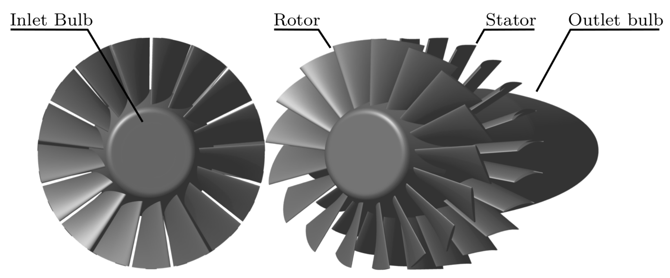
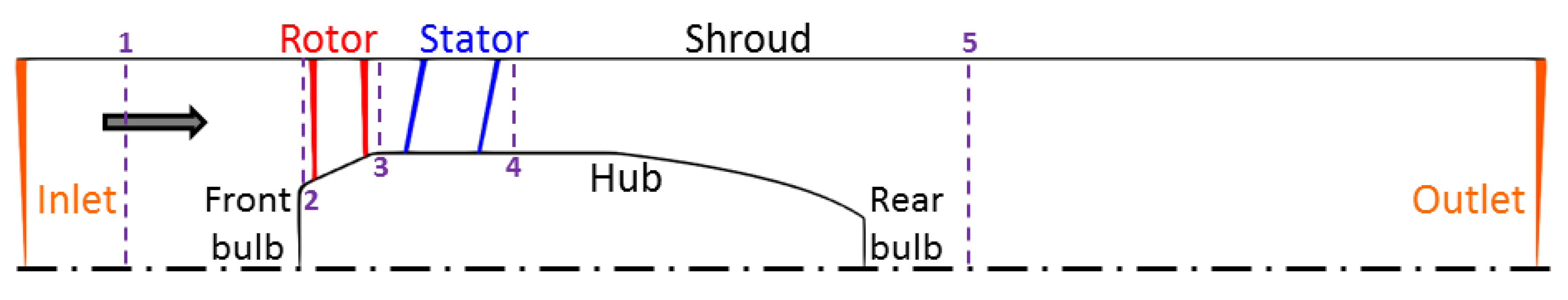
2. Test Case
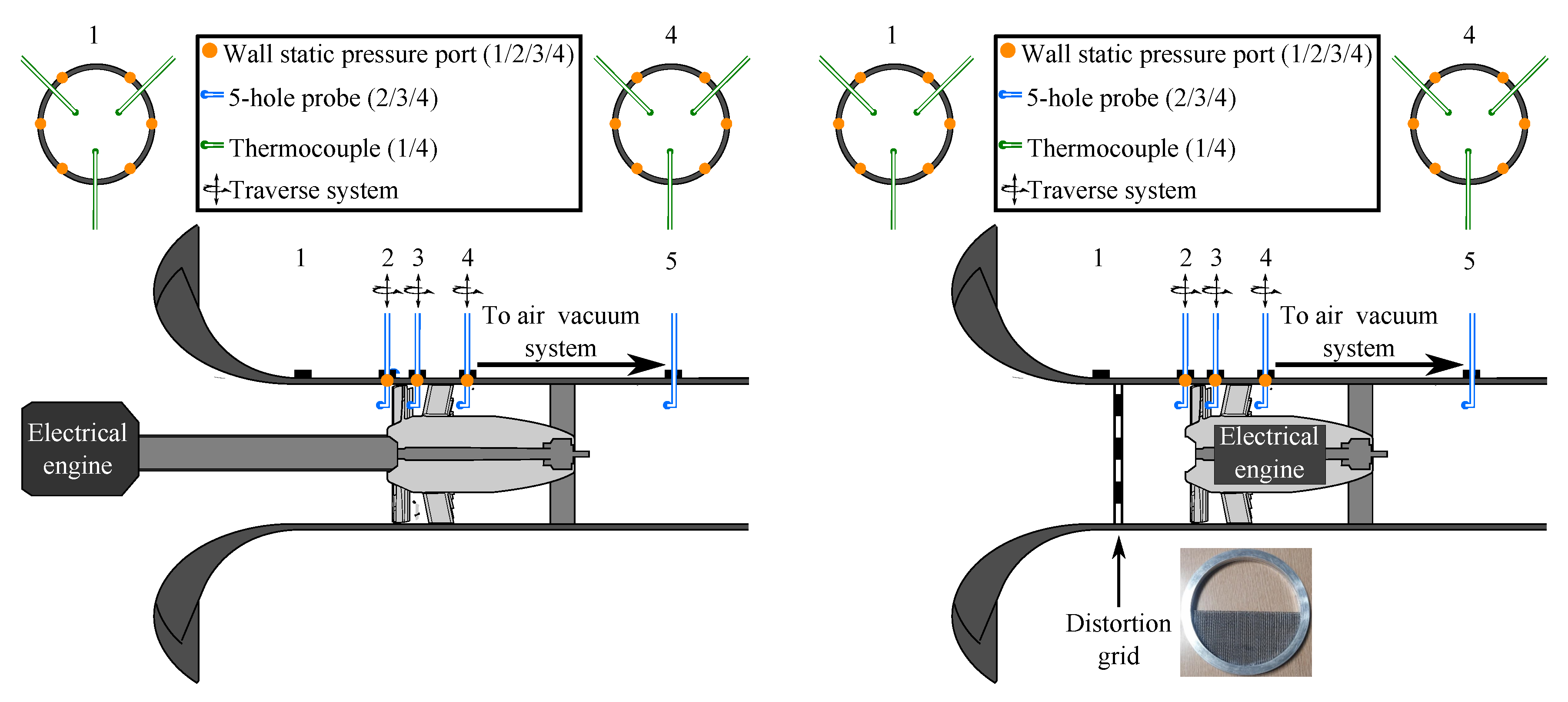
2.1. Test Rig
- Where the test rig is equipped with an asynchronous electric engine, which is located far from the test sections; this configuration corresponds to uniform upstream flow conditions (Figure 2, left).
- Where another electric engine is inserted in the fan body, so that there is no shaft outside of the body and distortion grids can be placed upstream of the fan stage in order to create nonuniform flow conditions (Figure 2, right).
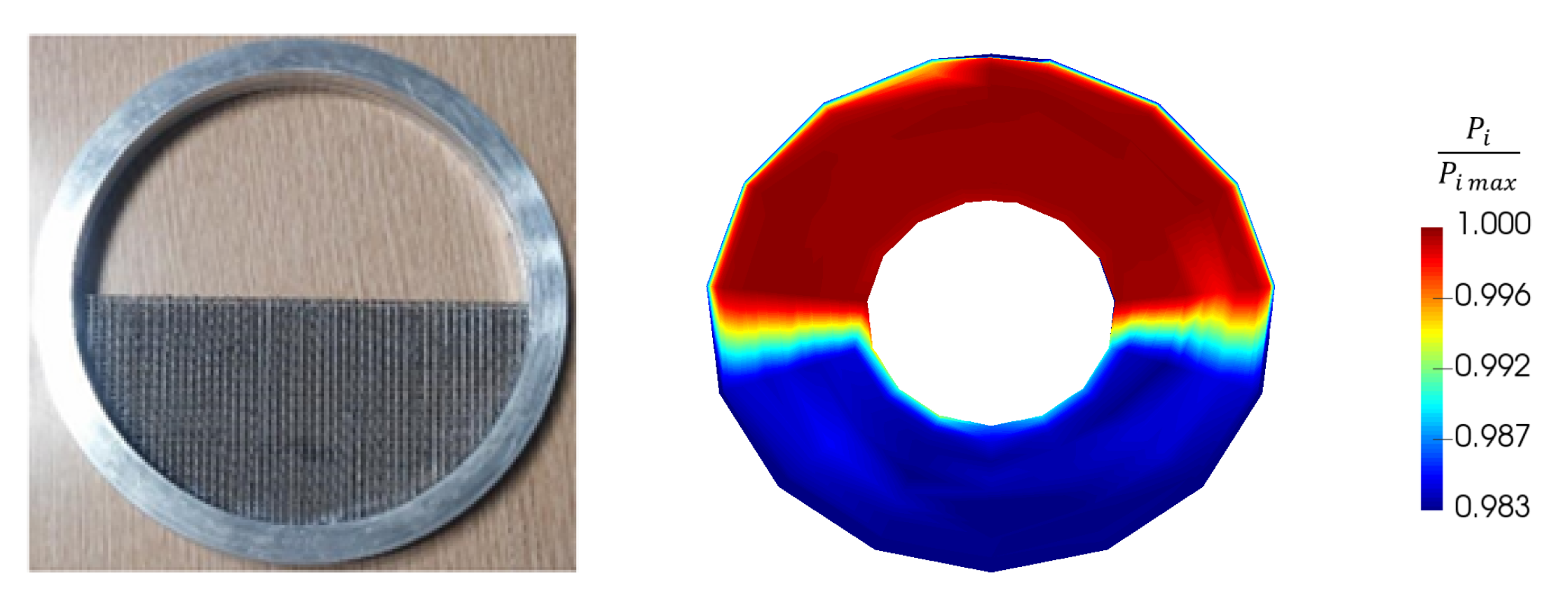
2.2. Distortion Grid
2.3. Instrumentation
3. Numerical Setup
3.1. URANS Simulations
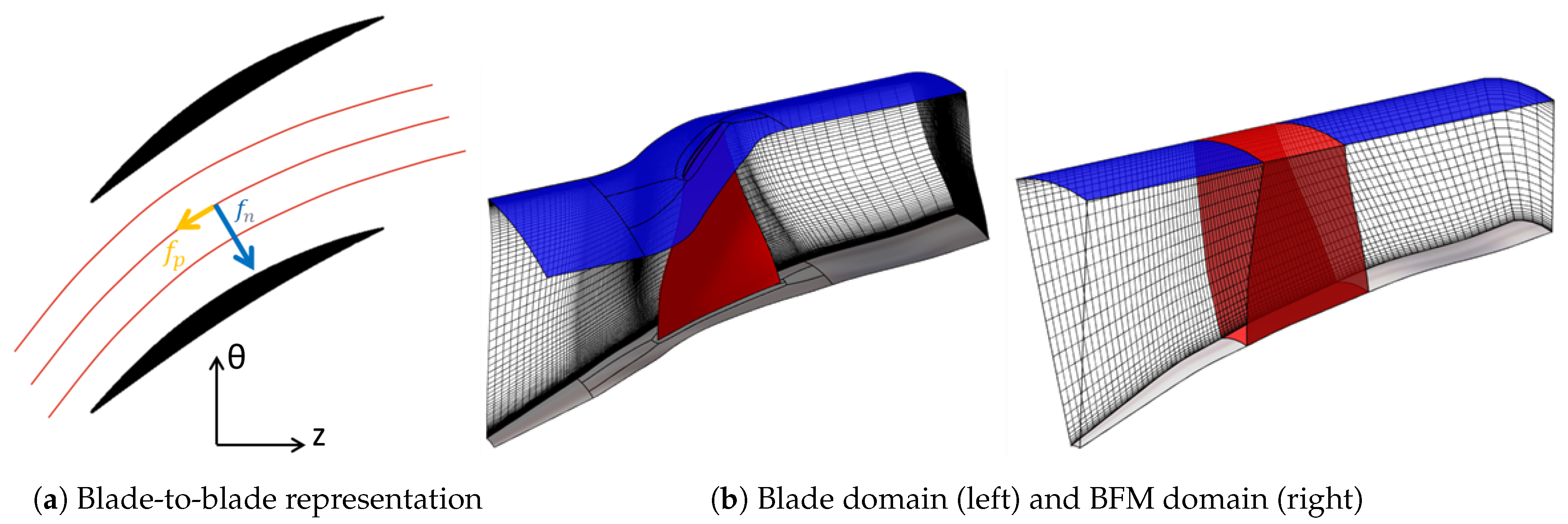
3.2. Body Force Methodology
- A force normal to the relative flow field, , which is responsible for the turning.
- A force parallel to the relative flow field, , which generates losses.
- The 3D mesh is simply obtained by extruding a 2D meridional mesh in the azimuthal direction; not meshing the boundary layers around the blades yields a very low cell count.
- More importantly, this method enables one to deal with distorted inflow while keeping a steady resolution, which considerably decreases the associated CPU cost.
- Finally, the general formulation is very flexible since the expressions of and are user-defined and can easily be adapted to the problem at hand. The local definition of the two force components also lets some room for extra calibrations, which can rely either on preliminary BFM simulations or on more accurate RANS results.
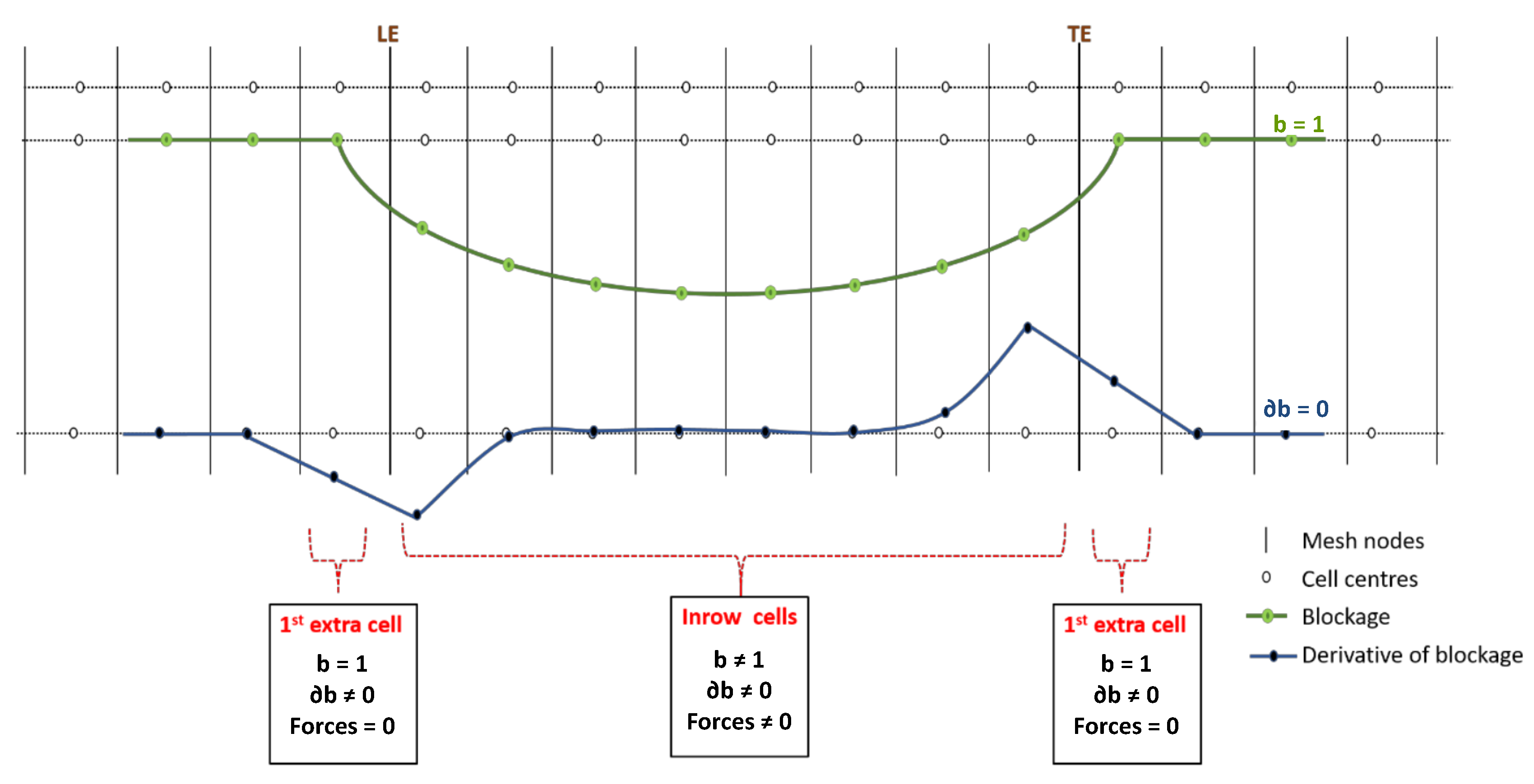
- Metal blockage effects are added according to Equation (5).
- A compressibility correction in the normal force definition was added. It has no visible effect in the present case, given the low pressure ratio involved. However, this correction has proven to be valuable in transonic configurations according to Thollet’s work [14].
- A parallel force is also introduced, in order to account for the loss without any exterior data input. This term only relies on a local friction coefficient , derived from an empirical turbulent flat plate correlation, and a local chordwise Reynolds number . Of course, no specific phenomenon is expected to be captured, such as an endwall corner separation or shock wave–boundary layer interaction.
3.3. Numerical Distortion
4. Results and Analysis
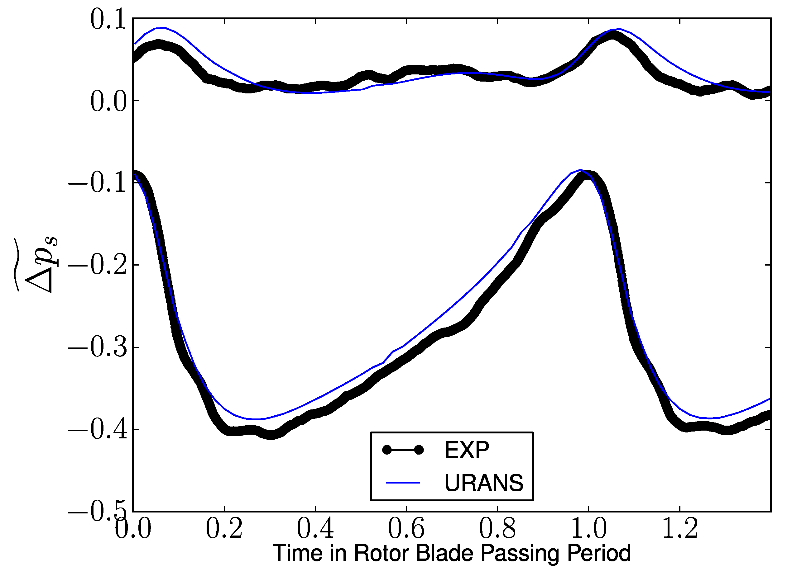
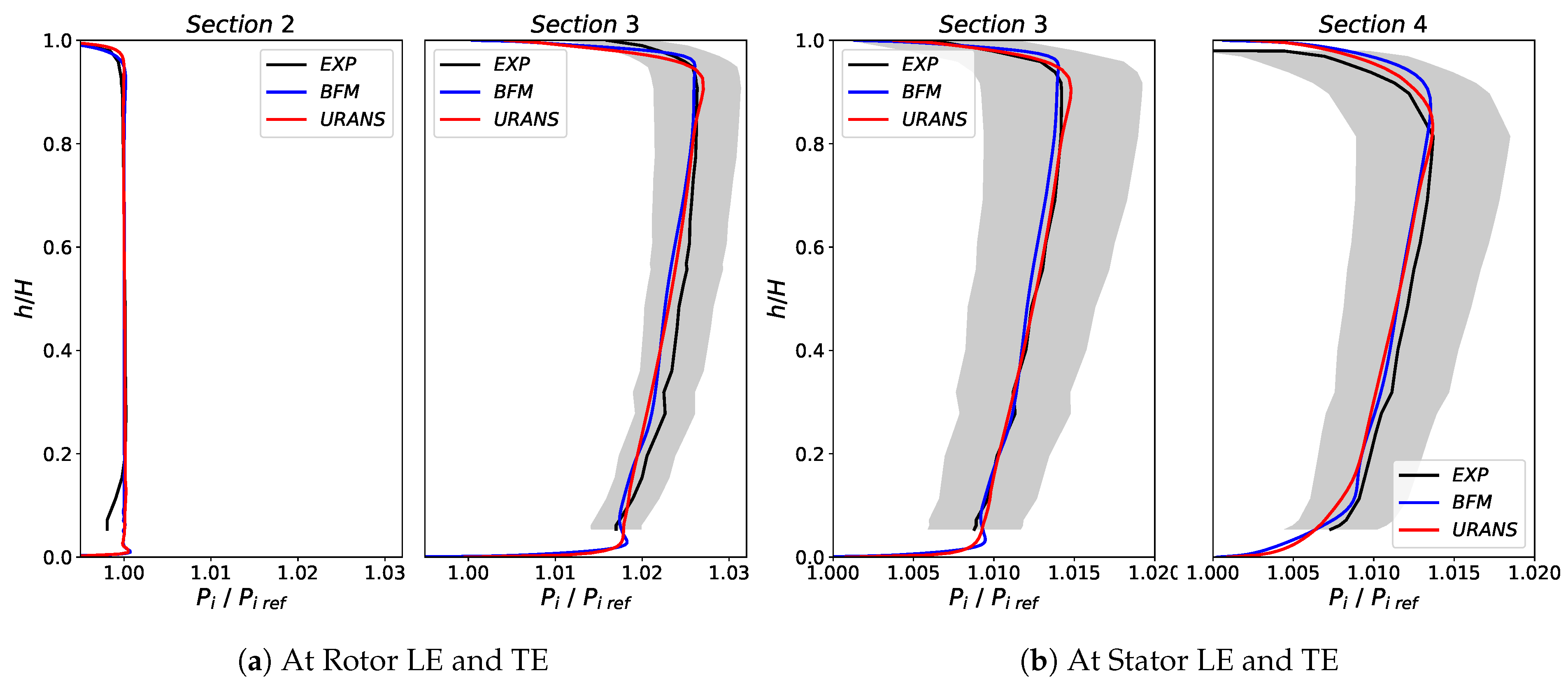
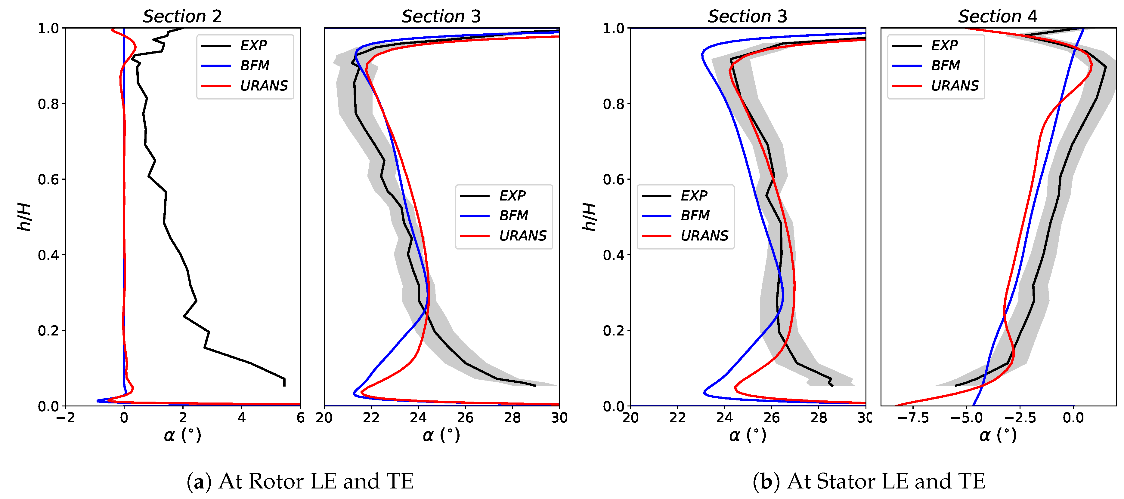
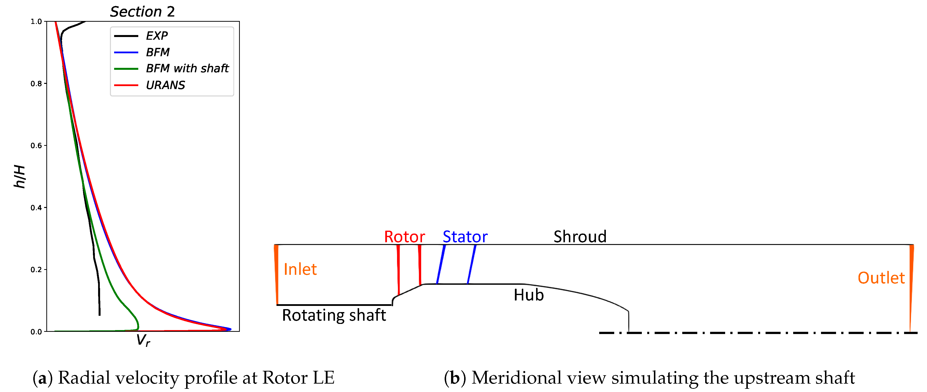
4.1. Validation of BFM in the Clean Case
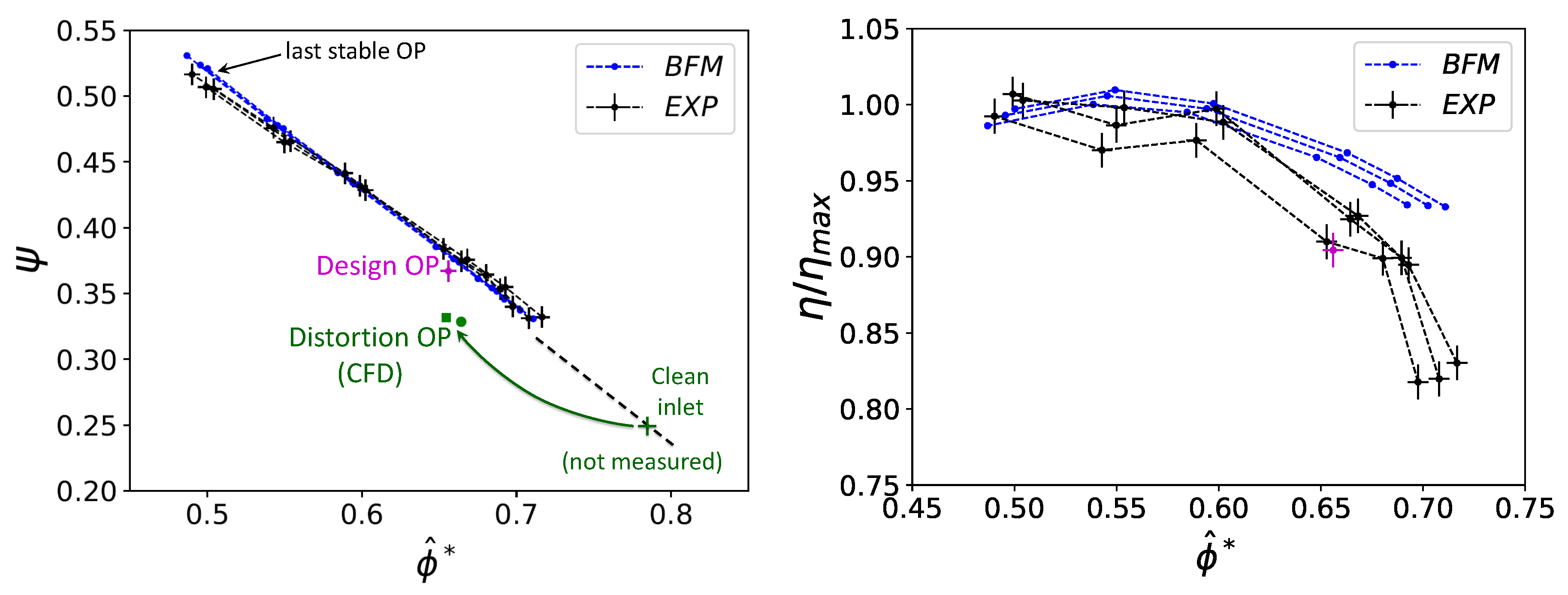
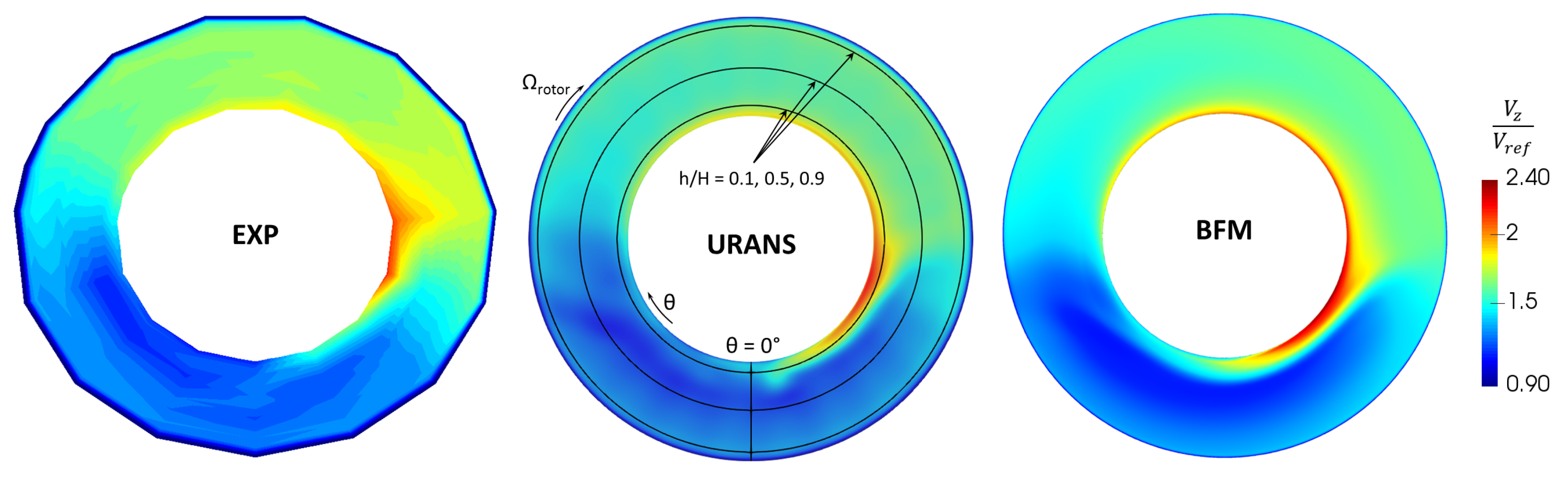
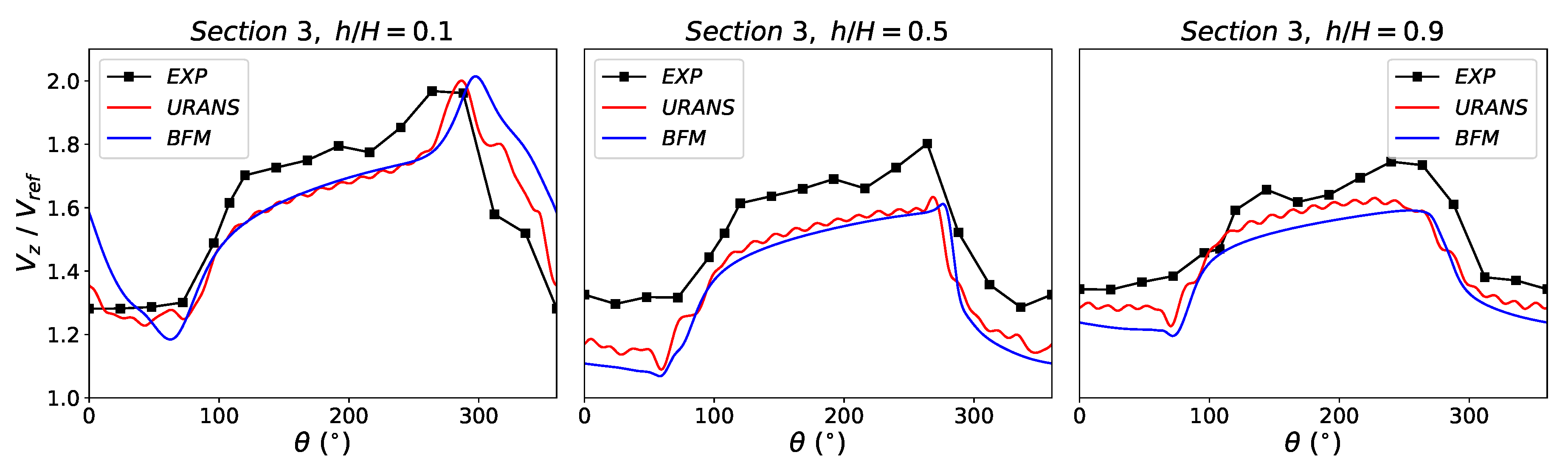
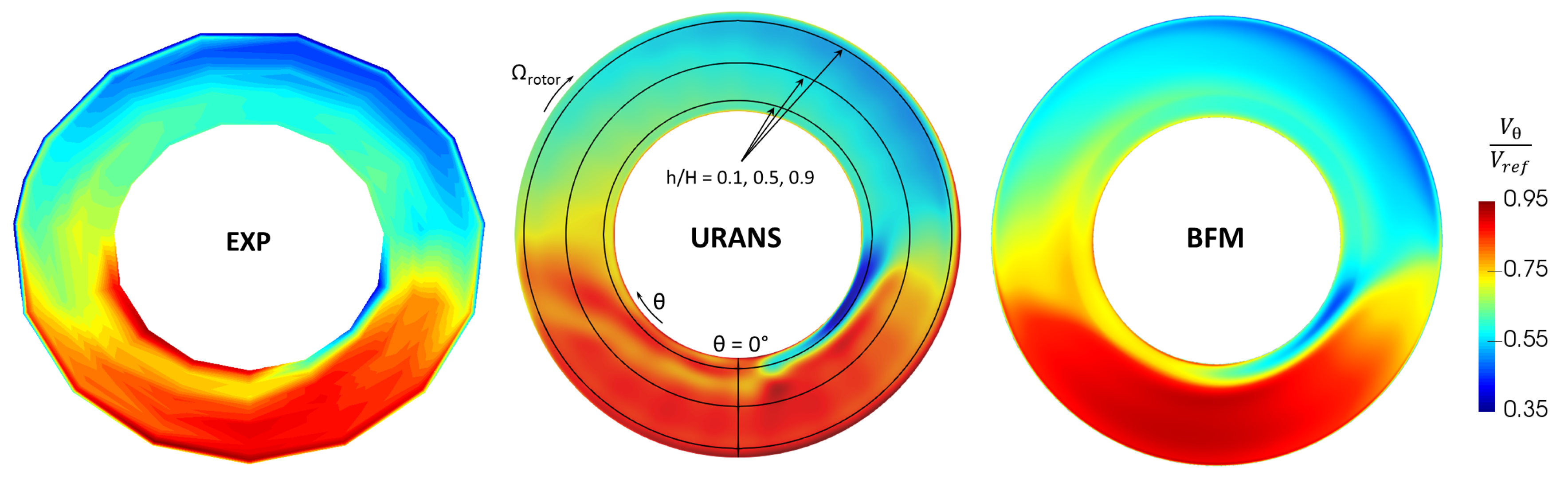
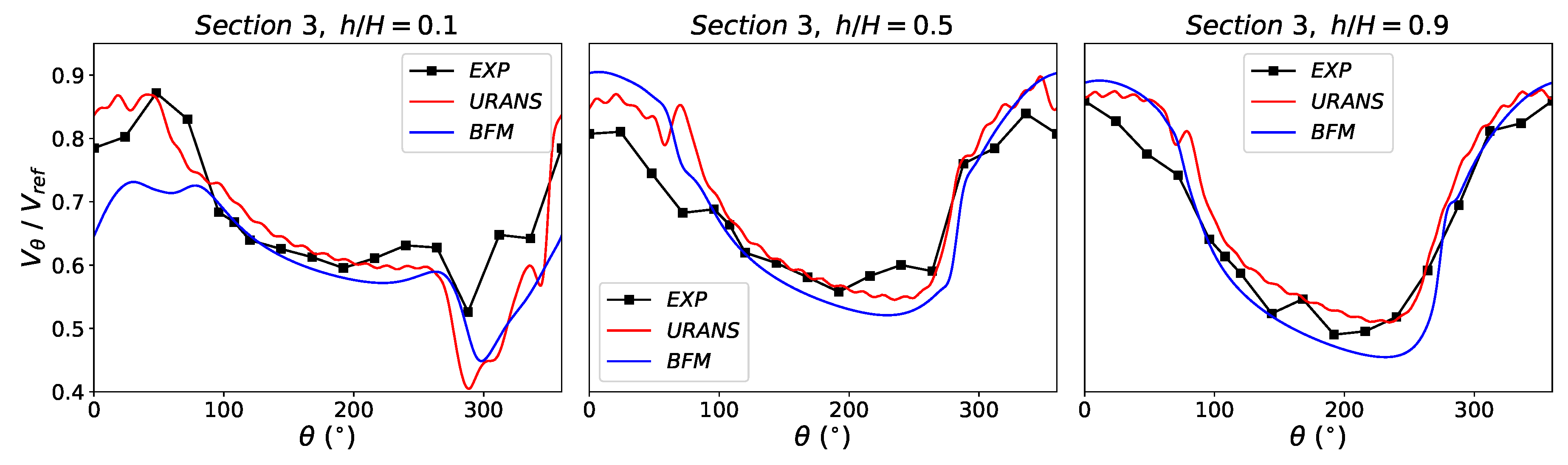
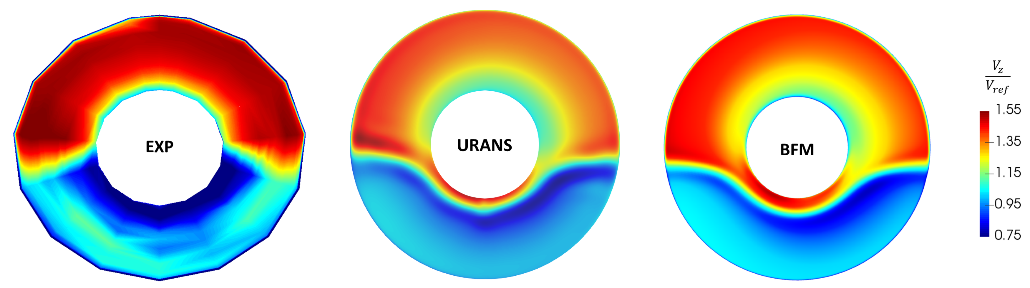
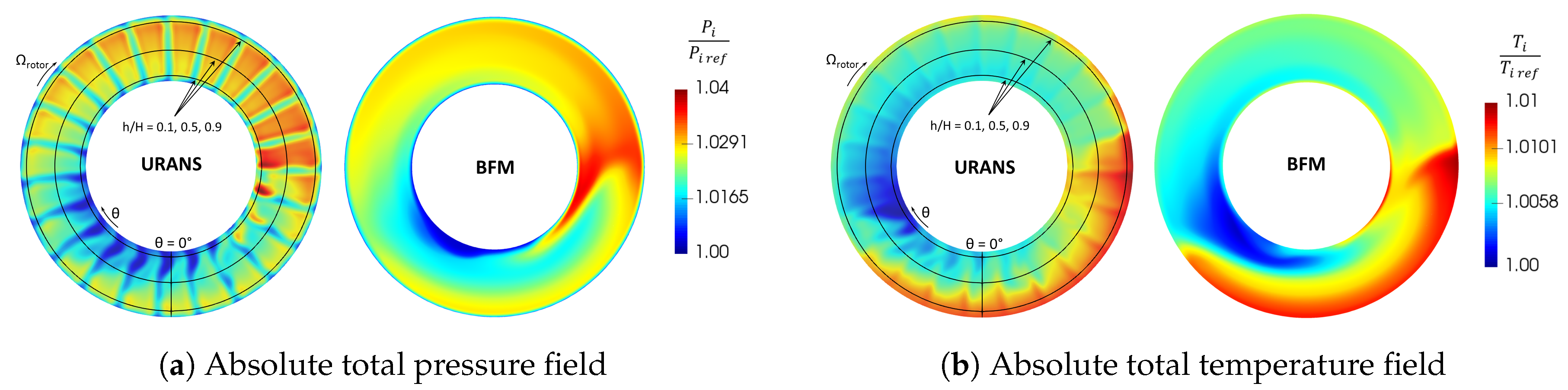
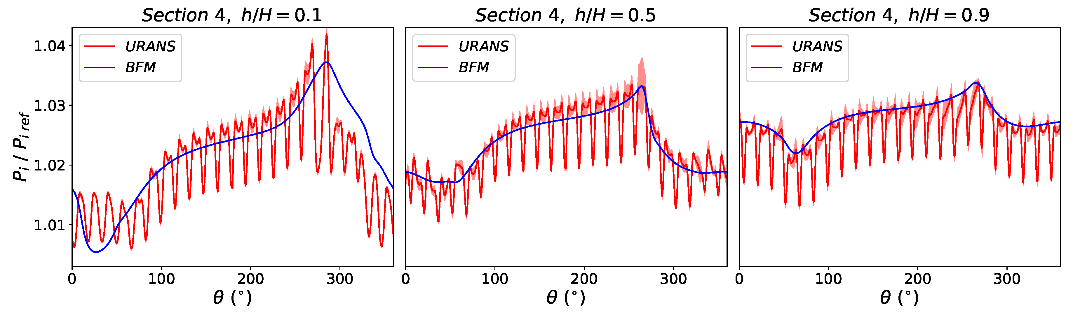
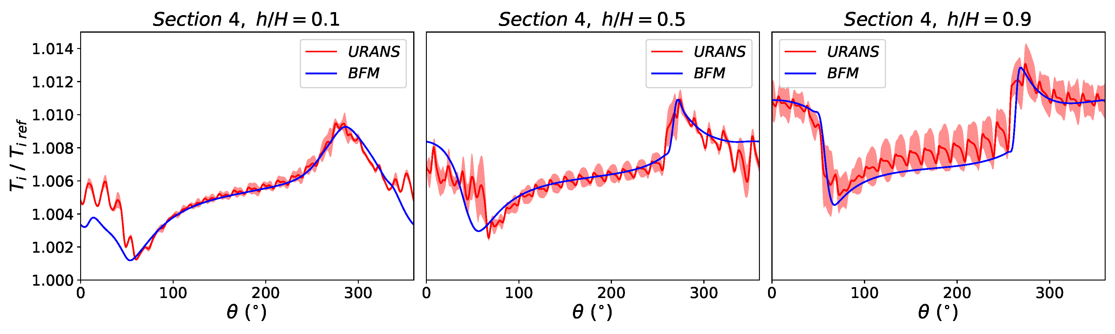
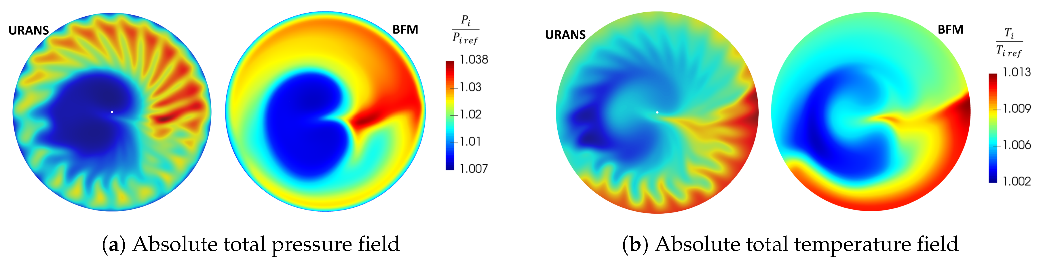
4.2. Evaluation of BFM with Distortion
5. Conclusions
Author Contributions
Funding
Acknowledgments
Conflicts of Interest
Abbreviations
| BLI | Boundary Layer Ingestion |
| BPF | Blade Passing Frequency |
| CFD | Computational Fluid Dynamics |
| CFL | Courant–Friedrichs–Lewy number |
| DTS | Dual time-stepping |
| LE | Leading Edge |
| PS | Pressure Side |
| SS | Suction Side |
| TE | Trailing Edge |
| URANS | Unsteady Reynolds-Averaged Navier–Stokes |
| Symbols | |
| b | blade metal blockage |
| , | blockage derivatives |
| vector normal to the blade camber surface | |
| s | blade pitch |
| N | blade count |
| W | relative velocity |
| V | absolute velocity |
| Reynolds number based on the chordwise direction | |
| friction coefficient | |
| kinematic viscosity | |
| turbulent kinematic viscosity | |
| density | |
| D | fan diameter |
| rotational speed | |
| relative Mach number | |
| flow coefficient | |
| loading coefficient | |
| reduced flow coefficient | |
| body force per unit mass | |
| compressibility correction coefficient | |
| local deviation angle | |
| pressure ratio | |
| isentropic efficiency | |
| static pressure recovery | |
| total pressure loss | |
| specific heat ratio | |
| relative span height | |
| corrected mass flow rate | |
| azimuthal component of | |
| Superscripts | |
| assessed at the mean quadratic radius | |
| total-to-total | |
| Subscripts | |
| x, y, z | cartesian coordinates |
| z, r, | cylindrical coordinates |
| n | normal to the flow |
| p | parallel to the flow |
| i | stagnation quantity |
| 1, …, 5 | relative to Section 1, Section 2, Section 3, Section 4 and Section 5 |
References
- Uranga, A.; Drela, M.; Greitzer, E.M.; Hall, D.K.; Titchener, N.A.; Lieu, M.K.; Siu, N.M.; Casses, C.; Huang, A.C.; Gatlin, G.M.; et al. Boundary Layer Ingestion Benefit of the D8 Transport Aircraft. AIAA J. 2017, 55, 3693–3708. [Google Scholar] [CrossRef]
- Hall, D.; Greitzer, E.; Tan, C. Analysis of fan stage conceptual design attributes for boundary layer ingestion. J. Turbomach. 2017, 139, 071012. [Google Scholar] [CrossRef]
- Gunn, E.; Hall, C. Aerodynamics of boundary layer ingesting fans. ASME Turbo Expo 2014: Turbine Technical Conference and Exposition; American Society of Mechanical Engineers: New York, NY, USA, 2014; p. V01AT01A024. [Google Scholar]
- Kim, H.; Liou, M.S. Flow simulation and optimal shape design of N3-X hybrid wing body configuration using a body force method. Aerosp. Sci. Technol. 2017, 71, 661–674. [Google Scholar] [CrossRef]
- Ortolan, A. Aerodynamic Study of Reversible Axial Fans with High Compressor/Turbine Dual Performance. Ph.D. Thesis, ISAE-SUPAERO, Toulouse, France, 2017. [Google Scholar]
- Binder, N.; Courty-Audren, S.K.; Duplaa, S.; Dufour, G.; Carbonneau, X. Theoretical Analysis of the Aerodynamics of Low-Speed Fans in Free and Load-Controlled Windmilling Operation. J. Turbomach. 2015, 137, 101001. [Google Scholar] [CrossRef]
- Ortolan, A.; Courty-Audren, S.K.; Lagha, M.; Binder, N.; Carbonneau, X.; Challas, F. Generic Properties of Flows in Low-Speed Axial Fans Operating at Load-Controlled Windmill. J. Turbomach. 2018, 140, 081002. [Google Scholar] [CrossRef]
- Cambier, L.; Gazaix, M. elsA—An efficient object-oriented solution to CFD complexity. In Proceedings of the 40th AIAA Aerospace Sciences Meeting & Exhibit, Reno, NV, USA, 14–17 January 2002; p. 108. [Google Scholar]
- Gourdain, N. High-Performance Computing of Gas Turbine Flows: Current and Future Trends; HDR, École Centrale de Lyon: Écully, France, 2011. [Google Scholar]
- Marble, F. Three Dimensional Flow in Turbomachines. InHigh Speed Aerodynamics and Jet Propulsion; Princeton University Press: Princeton, NJ, USA, 1964; pp. 83–166. [Google Scholar]
- Gong, Y.Y. A Computational Model for Rotating Stall and Inlet Distortions in Multistage Compressors. Ph.D. Thesis, Massachussets Institute of Technology, Cambridge, MA, USA, 1998. [Google Scholar]
- Peters, A. Ultra-Short Nacelles for Low Fan Pressure Ratio Propulsors. Ph.D. Thesis, Massachussets Institute of Technology, Cambridge, MA, USA, 2014. [Google Scholar] [Green Version]
- Defoe, J.J.; Spakovszky, Z.S. Shock Propagation and MPT Noise From a Transonic Rotor in Nonuniform Flow. J. Turbomach. 2012, 135, 011016. [Google Scholar] [CrossRef] [Green Version]
- Thollet, W. Body Force Modeling of Fan—Airframe Interactions. Ph.D. Thesis, ISAE-SUPAERO, Toulouse, France, 2017. [Google Scholar]


| Diameter | mm |
| Rotor blade count | |
| Stator blade count | |
| Design rotational speed | rpm |
| Design reduced flow coefficient | |
| Design stage loading coefficient | |
| Reynolds number | |
| Axial Mach number | 0.1–0.2 |
| BFM-URANS |
© 2019 by the authors. Licensee MDPI, Basel, Switzerland. This article is an open access article distributed under the terms and conditions of the Creative Commons Attribution (CC BY) license (http://creativecommons.org/licenses/by/4.0/).
Share and Cite
Benichou, E.; Dufour, G.; Bousquet, Y.; Binder, N.; Ortolan, A.; Carbonneau, X. Body Force Modeling of the Aerodynamics of a Low-Speed Fan under Distorted Inflow †. Int. J. Turbomach. Propuls. Power 2019, 4, 29. https://0-doi-org.brum.beds.ac.uk/10.3390/ijtpp4030029
Benichou E, Dufour G, Bousquet Y, Binder N, Ortolan A, Carbonneau X. Body Force Modeling of the Aerodynamics of a Low-Speed Fan under Distorted Inflow †. International Journal of Turbomachinery, Propulsion and Power. 2019; 4(3):29. https://0-doi-org.brum.beds.ac.uk/10.3390/ijtpp4030029
Chicago/Turabian StyleBenichou, Emmanuel, Guillaume Dufour, Yannick Bousquet, Nicolas Binder, Aurélie Ortolan, and Xavier Carbonneau. 2019. "Body Force Modeling of the Aerodynamics of a Low-Speed Fan under Distorted Inflow †" International Journal of Turbomachinery, Propulsion and Power 4, no. 3: 29. https://0-doi-org.brum.beds.ac.uk/10.3390/ijtpp4030029