Article

Numerical Investigation of the Performance Impact of Stator Tilting Endwall Designs on a Mixed Flow Turbine

1
Department of Energy Technology, KTH Royal Institute of Technology, SE-100 44 Stockholm, Sweden
2
School of Mechanical and Aerospace Engineering, Queen’s University Belfast, Belfast BT9 5AH, UK
3
Department of Mechanical, Manufacturing and Biomedical Engineering, Trinity College Dublin, Dublin 2, Ireland
*
Author to whom correspondence should be addressed.
Int. J. Turbomach. Propuls. Power 2021, 6(2), 14; https://0-doi-org.brum.beds.ac.uk/10.3390/ijtpp6020014
Submission received: 16 December 2020 / Revised: 17 May 2021 / Accepted: 24 May 2021 / Published: 28 May 2021

Abstract

:
This paper numerically investigates stator endwall designs for a mixed flow turbine. One key design parameter studied is the tilting angle of the stator endwall. By examining stator designs with different tilting angles, the aim of this paper is to improve the efficiency of the studied mixed flow turbine at low velocity ratio working conditions. The performance curve at the design speed was chosen for the comparison between the baseline design and the tilted endwall designs. First, the numerical predictions for the baseline design were validated with experimental data. Then, to understand the mechanism of the performance variation between the different designs, the internal flow field was analyzed in detail. It was found that the tilting stator endwall could form a geometric “kink” in the endwall profiles. On the shroud side, certain designs with such kink caused local flow separations upstream the rotor leading edge. This separation could have the effect of reducing the intensity of the tip leakage vortex and the exit kinetic energy losses at the rotor outlet and may also improve the performance of the exhaust diffuser. As a result, the peak of the efficiency curve shifted toward lower velocity ratio. If the turbine stage incorporated a downstream exhaust diffuser, the optimal design in this study showed a shift of the velocity ratio of the peak efficiency point from 0.62 to 0.60 compared with the baseline. The maximum efficiency improvement was 1.3% points, which occurred at low velocity ratio. Meanwhile, the peak efficiency was 0.2% points higher than the baseline. If the exhaust diffuser was removed, a similar shift of the efficiency curve was observed but less efficiency gain was achieved at the low velocity ratio condition. A preliminary unsteady simulation was also conducted for the optimal design in this study.

1. Introduction

A mixed flow turbine (MFT) is a promising alternative design to a radial flow turbine (RFT) in turbocharger applications. It introduces several potential benefits to the turbocharging system. First, a well-designed MFT can have the advantage of lower rotor inertia than an RFT, which will improve the transient performance of the coupled engine-turbocharger system [1]. Second, for high specific speed designs, higher efficiency can be achieved from MFT [2]. Third, the forward-curved leading edge of an MFT leads to a better incidence condition and thus a better performance for high-stage-loading designs [3]. Lastly, an MFT can improve the energy recovery from the exhaust gas of the engine in a pulse turbocharging because of the potentially better efficiency at low velocity ratios [4]. These aforementioned benefits, especially the last two, provide a strong motivation for the research of MFT design. Therefore, a further explanation of the last two benefits is given in the following paragraphs.
The efficiency of RFTs can be correlated into a chart of RFT designs with different flow coefficients and stage-loading coefficients [5]. From this chart, it can be seen that the peak efficiency island lies below the stage-loading coefficient 1.0. One possible reason is that the incidence angle becomes positive as the stage-loading coefficient exceeds 1.0 [3]. This positive incidence angle deviates from the optimum incidence region of −20° to −40° [6] for an RFT, which may lead to an excessive increase of the incidence loss. In contrast, MFTs can reduce this positive incidence angle by introducing a non-zero inlet blade angle and thereby improving the performance at high-stage-loading conditions. Assuming an RFT and an MFT have the same rotor tip speed and the same stage efficiency, then a high-stage-loading coefficient also indicates a high-stage pressure ratio. That is to say the MFT may tend to have an improved performance at high-stage pressure ratio conditions, which introduces the next advantage of MFT in pulse turbocharging applications.
Figure 1a illustrates the pulsating variation of the inlet total pressure and the power output of the turbine in an engine cycle. In general, the turbine output power follows the variation of the total pressure. The peak of the turbine inlet total pressure is marked as point P, while the cycle endpoints are marked as points L. Since the turbine outputs more instant power at point P, an improved performance of turbine at high inlet total pressure conditions could lead to better utilization of the instant peak power. From a steady-state perspective, assuming the same rotor tip speed, U, is used for different designs, the pressure ratios of points P and L can correspond to respective U/C values in a turbine performance map, as shown in Figure 1b. To achieve a higher efficiency at point P, one possible strategy is to shift the efficiency curve toward the low U/C side. Although this shift may lead to a lower efficiency at point L, it has little significance to the cycle power output due to the low available energy at that point [4]. Such shifts of efficiency curve have been documented in published articles for MFT designs compared to its RFT counterparts. However, a recent study [1] showed that such shifts may result only from the smaller rotor inlet radius chosen to calculate the rotor tip speed U, instead of an actual performance improvement at high-pressure ratio conditions. It means that the radius to calculate U must be consistent when comparing different designs in a performance map like Figure 1b and a further investigation is still needed to improve the performance of MFT designs at high-pressure ratio conditions. In this study, since the same MFT rotor was used for all numerical simulations and the same inlet mean radius was used to calculate U/C, the choice of the radius to calculate U was consistent through the study and therefore comparisons like Figure 1b were meaningful within this study.
The performance of an MFT is determined by the detailed design of each component. One important component of an MFT is the stator endwall upstream of the rotor, as shown in Figure 2. For the stator endwall, the main design parameter is the tilting angle (δ in Figure 2b). There were several vaneless or vaned stator design examples in literature. From these designs, it was found that the tilting design was preferred for vaneless stators and the tilting angle could be either perpendicular to the rotor leading edge [7] (illustrated as Figure 2a) or tangential to the downstream endwall profile [8] (illustrated as Figure 2b). But for a vaned stator design, a radial stator endwall (illustrated as Figure 2c) was argued to be more practical [9]. These different stator endwall layouts can affect the aerodynamic performance of an MFT. Lee et al. compared the performance of a tilted and a radial vaneless volute for the same MFT. It was found the tilted volute could increase both the steady-state performance [10] and the cycle-averaged performance under pulsating working conditions [11]. A follow-up study investigated the effect of inlet spanwise flow distributions on the aerodynamic performance by implementing different distributions on a radial and a tilted stator layouts [12]. However, a direct comparison of those two stator layouts was not achievable due to the lack of aerodynamic similarity [12]. Morrison et al. [13] investigated the effect of inlet flow cone angle on the performance of an MFT, as an indirect way to investigate the stator endwall tilting designs. The upstream stator parts were not included in the numerical simulation. Instead, the different inlet flow cone angles were implemented as the inlet boundary condition. The highest efficiency occurred near the radial inlet condition, instead of the tilting one. This result caused an inconsistency of general conclusions between the works of different researchers. Due to the contradicting results and the diversity of designs, research work is still needed to clarify the effect of a tilting stator endwall on the general performance of an MFT.
As can be seen from Figure 2a,c, the non-tangential designs may generate a “kink” in the endwall profile, as shown in the enlarged view in Figure 2a. To the authors’ knowledge, the effect of such a kink structure has never been examined for MFTs, even though its positive effect on the aerodynamic performance has been documented for axial turbines as a stepped casing or axisymmetric endwall contouring. In [14], the detailed analysis of the flow field presented local flow separation regions caused by the stepped casing. Despite the additional endwall losses from the separation, the stage performance was still improved due to the reduction of the tip leakage losses. However, as mentioned in [15], the tip leakage mechanism in an RFT is different from an axial turbine because of the variation of radius on the shroud side. Therefore, there is no guarantee that such improvement in [14] will also be seen in an RFT. As for MFT, since this variation of radius on the shroud side also exists, it is worthwhile to examine its tip leakage flow structure and the influence of such a kink structure on the aerodynamic performance of an MFT.
This paper, in a systematic manner, numerically investigates the effect of stator tilting endwalls on the aerodynamic performance of a typical MFT with a vaned stator. The baseline MFT design is first introduced in Section 2.1. Since computational fluid dynamics (CFD) was used as the research tool to analyze the different tilting designs in this study, Section 2.2 describes the CFD method followed by the validation of the method by comparing the CFD results with the experimental data. Section 2.3 presents the design method and the design matrix of the stator tilting endwall. To simplify the design process, the design domain was limited to the vaneless space between the nozzle exit and the rotor inlet. The tilting angle δ of the endwall was the main design parameter. This angle δ varied over a wide range on both the hub and the shroud side. In terms of the results and discussions (Section 3), the general performances for all designs in the matrix are first presented (Section 3.1). From these general performances, the overall trend was established and the optimal design and several other interesting designs were identified among the matrix. To explain the significant performance variations, a loss breakdown and a detailed flow field analysis were conducted at the highest pressure ratio working point (Section 3.2), and at the peak efficiency and the lowest pressure ratio working points (Section 3.3) on the performance curve. The focus was given to the effect of the endwall kink on the tip leakage vortex and on other internal flow features. Additionally, the optimal stator tilting endwall design in this study was evaluated in a stage layout without the exhaust diffuser (Section 3.4) and unsteady CFD simulations were conducted to confirm the performance improvement (Section 3.5), followed by the conclusions (Section 4).

2. Materials and Methods

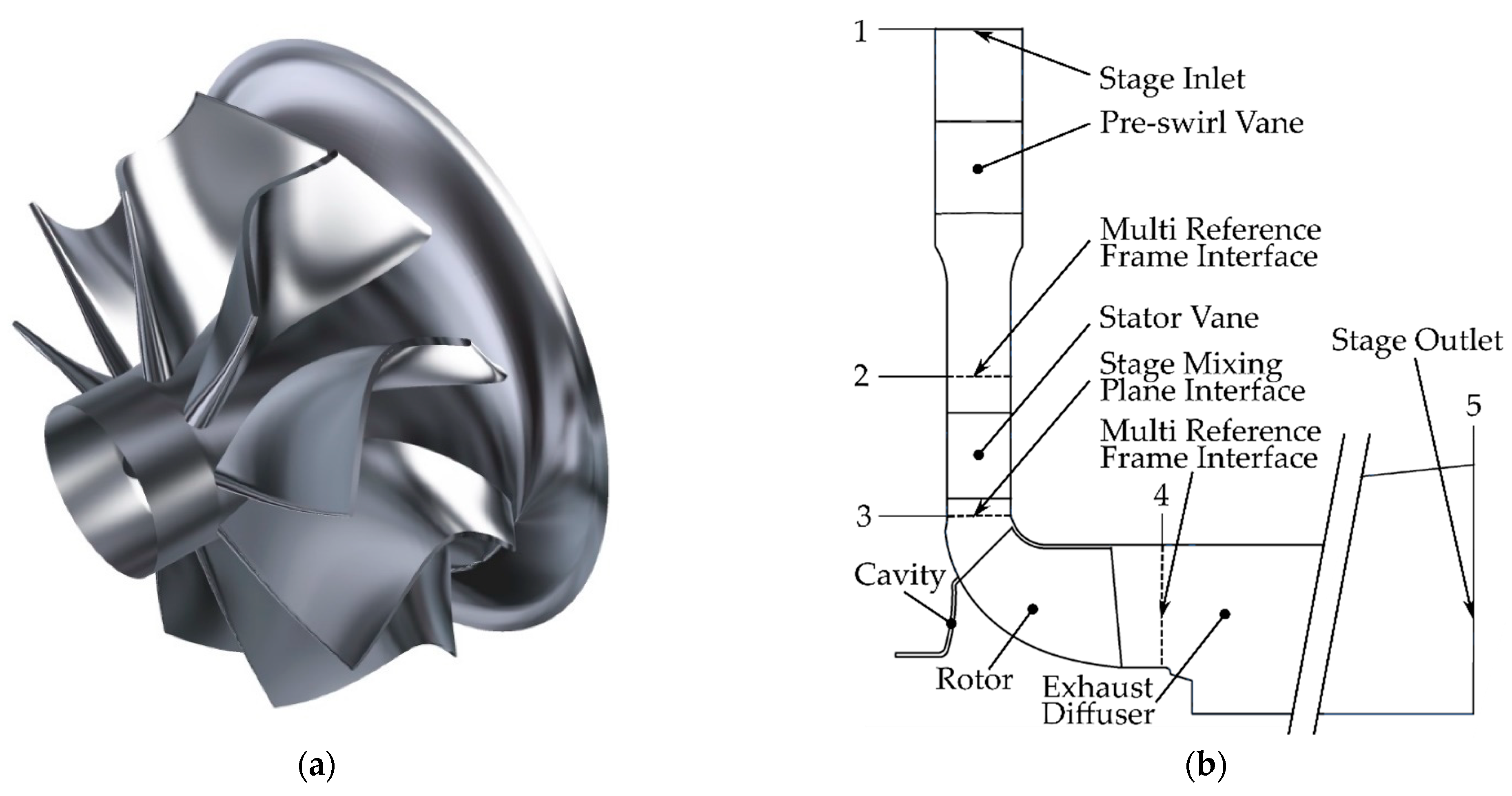
2.1. Baseline Turbine Stage

The baseline MFT stage studied in this paper was developed at Queen’s University Belfast (QUB) [1,16]. The MFT rotor design was based on a state-of-art RFT in a turbocharger application. It had an inlet tip diameter of 90 mm and a blade count of 9. The MFT rotor had a blade cone angle of 45° and a nominal constant inlet blade angle of 20° (Figure 3a). The aerodynamic performance of the MFT was experimentally investigated on the cold flow turbine test rig at QUB. Different from a typical turbocharger, this test rig had no volute but used pre-swirl vanes and straight stator vanes to generate the tangential flow at the rotor inlet. The meridional view of the baseline stage is presented in Figure 3b. This approach led to an advantage in CFD validation because a single-passage model can be used and thereby greatly reducing the computational effort. More details about this test rig can be found in [17].
This baseline MFT was numerically studied in [17], where it was found that the tip leakage vortex (TLV) was one of the main loss sources in the flow field. But it was also noted in [17] that the losses due to the TLV could be reduced by modifying the upstream stator vane with a leaned design, which led to significant improvement of the turbine performance. Therefore, the TLV has been carefully considered in this study when different stator tilting endwall designs were implemented.

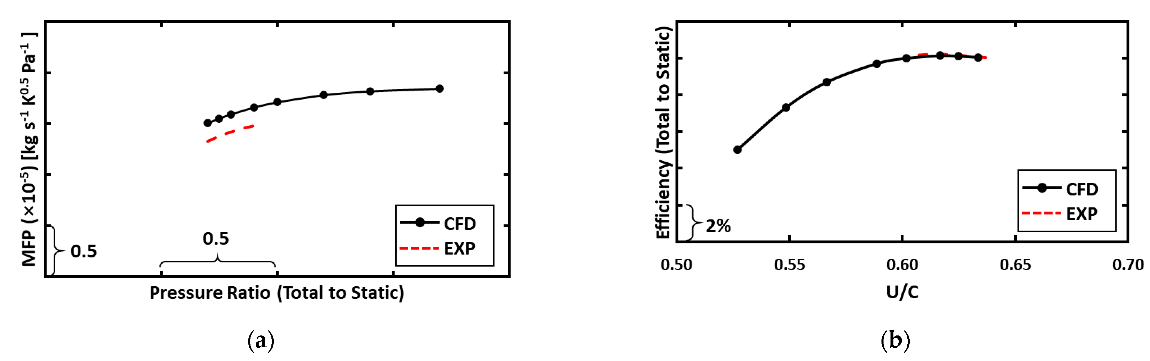
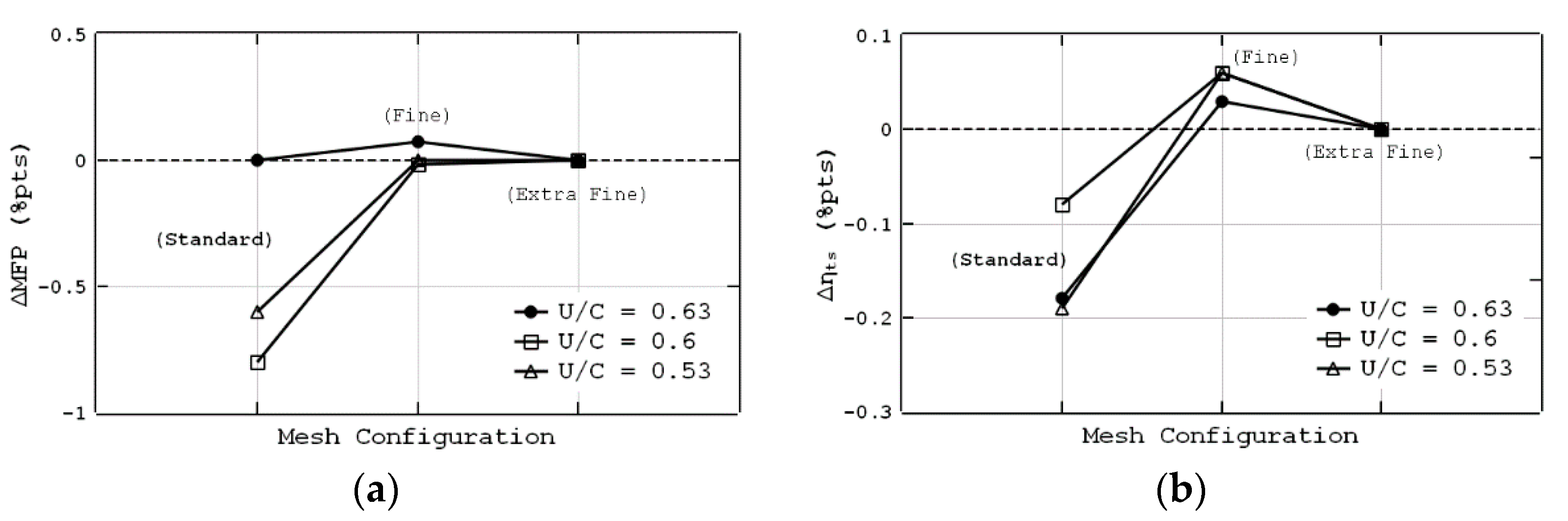
2.2. CFD Modeling Method and Validation

The stator tilting endwall designs were numerically analyzed in this paper using the commercial CFD software ANSYS 19.5-CFX. The same computational domains as [17] were utilized, as shown in Figure 3b. To reduce the computational effort, steady-state single passage domains were used and they were connected by interfaces. The meshes of the pre-swirl vane, the cavity and the exhaust diffuser domains were kept the same as [17]. Meanwhile, for different stator tilting endwall designs, the stator meshes were generated in NUMECA-Autogrid (Turbo 132) software and the original rotor mesh was modified in NUMECA-IGG (Turbo 132). The mesh element count was 321k for the stator vane region and 1475k for the rotor region. According to the mesh independence study in [17], the current mesh element should cause less than −0.1% points difference of efficiency compared with the finest grid in the independence study. It should be noted here the mesh independence study in [17] was only used for the baseline design. Due to the significant geometry change of stator tilting endwall designs, a separate mesh independence study was conducted for the optimal design in this study in Section 3.1. Since the shear stress transport (SST) turbulence model was employed, the meshes were refined close to the blade surface and other wall surfaces. The y+ value was maintained below 11 for all wall surfaces. In addition, the y+ value was also checked on the endwall surface near the shroud “kink” where the y+ value was maintained below 10 for all cases. These y+ values ensured that all near-wall flows were directly solved by the turbulence model. In terms of boundary conditions, a uniform total temperature and total pressure were implemented at the stage inlet and a plane-averaged static pressure at the stage outlet. The convergence criterion was that the root-mean-square (RMS) residual was below 1e-5 and the key parameters (i.e., efficiency, mass flow parameter (MFP) and pressure ratio) reached a steady-state value. The MFP and the efficiency from the CFD results were calculated based on the mass-averaged parameters at the inlet and outlet surfaces:
M F P = m T 01 P 01
η t s , s t a g e = 1 ( T 05 / T 01 ) 1 ( P 5 / P 01 ) ( k 1 ) / k
The CFD results of the aforementioned baseline model (Figure 3b) were compared with the experimental (EXP) data at the design speed as shown in Figure 4. In general, the CFD results were in good agreement with the experimental data. In the MFP diagram (Figure 4a), the CFD result had the same trends as the experimental one. The maximum deviation of MFP was found at the minimum pressure ratio point where a 3.4% over-prediction of the CFD result was seen. The same deviation was also documented in [17]. Through a literature study of [18,19,20,21,22], the maximum deviation of MFT between CFD results and test data was found within the range of 2–6%. As the current deviation fell within that range, the literature study added confidence to the current CFD method. The deviation of MFP in the current study resulted from the lack of the fillet structure in the CFD model, the experimental uncertainty of the mass flow measurement and the steady-state single passage CFD model. The effect of steady-state CFD model on the MFP could be seen in Section 3.5 of this study, where the results of steady and unsteady CFD models were compared. In the efficiency diagram (Figure 4b), the CFD result presented no noticeable deviation from the experimental data.

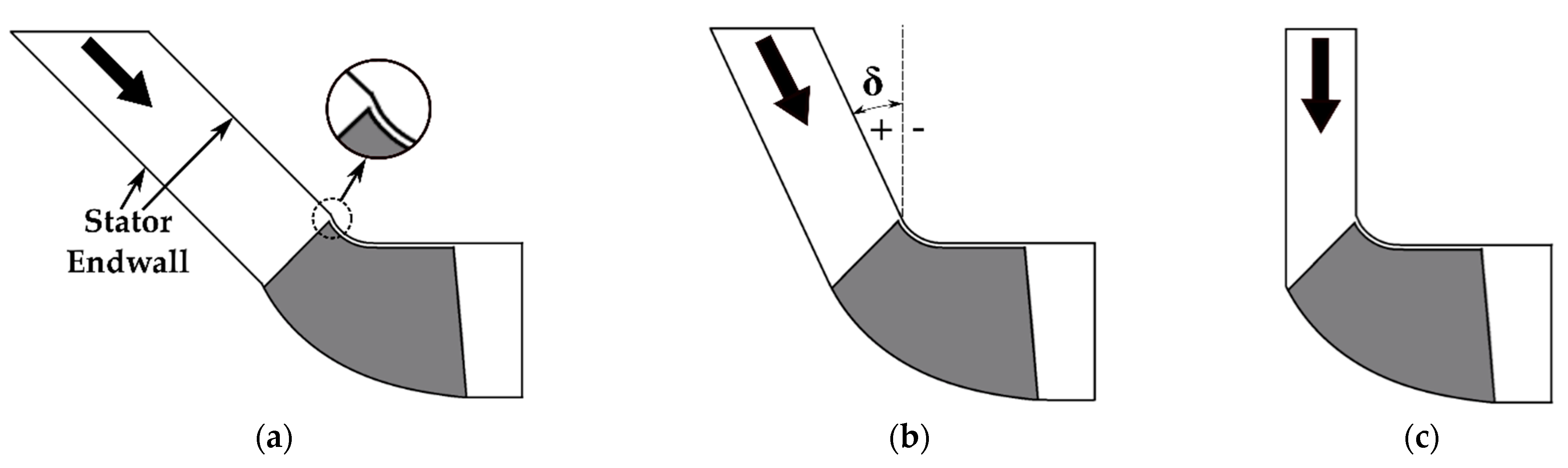
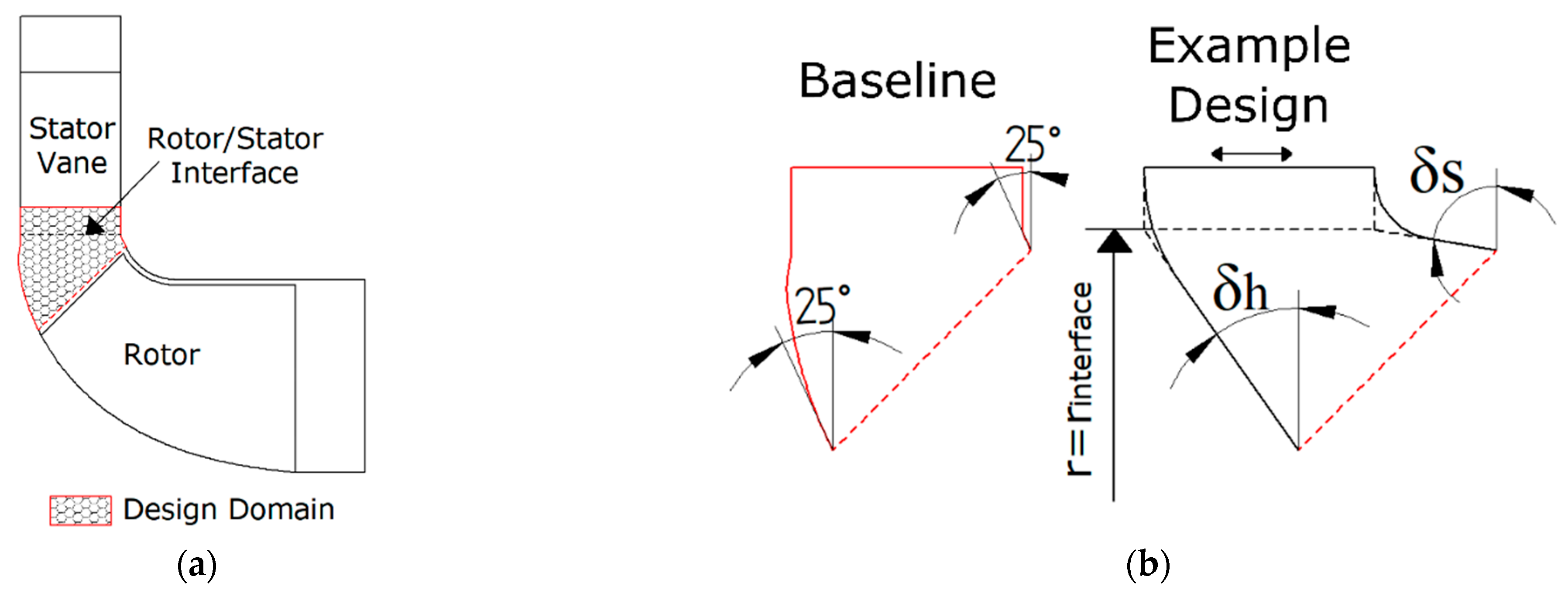
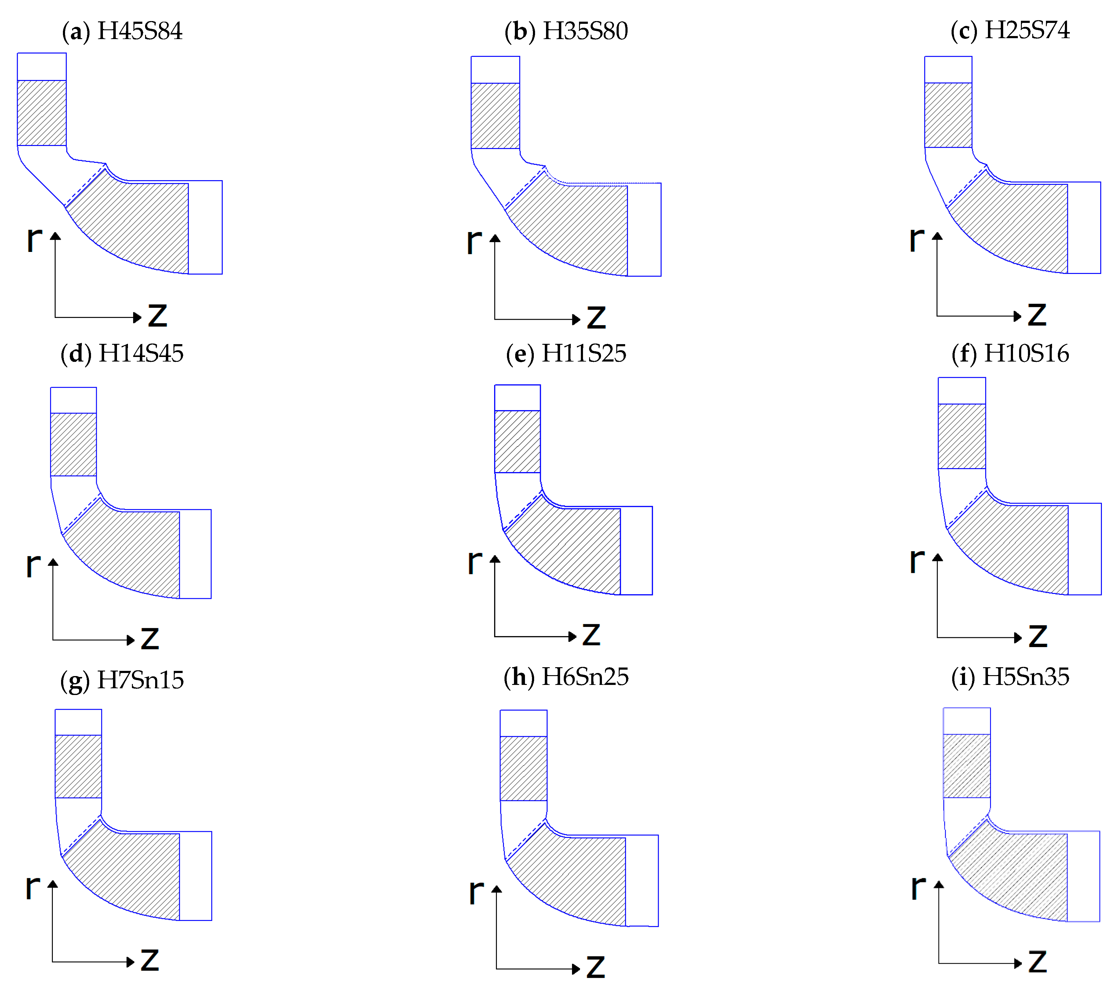
2.3. Design of Stator Tilting Endwall

All the CFD simulations in this study had the same domains, interface, and modeling setting as the baseline in Figure 3b. However, the geometry of the stator endwall was redesigned with different tilting angles. The design domain of the stator tilting endwall was limited to the vaneless space between the stator vane outlet and the rotor blade inlet, as shown in Figure 5a. Since there were no geometric modifications in the other domains, such as the pre-swirl vane, the back-disk cavity, and the exhaust diffuser, for simplification reason, only the stator and rotor domains are shown here to illustrate the stator tilting endwall designs. The rotor/stator interface was kept at the same radius for all the designs, namely rinterface. On the stator side, any design modifications were intentionally kept out of the stator vane domain. As a result, the geometry of the stator vane was exactly the same as the baseline. This simplified the design process by avoiding the re-design of the stator vane and a direct comparison between different designs was enabled based on the same upstream layouts. On the rotor side, a conical plane upstream the rotor leading edge was selected as the design domain boundary (red dashed line in Figure 5a). This constrain led to an unchanged mesh in the downstream rotor domain and an unchanged rotor tip clearance. It should be highlighted that the meshes at the design domain outlet were fully matched with the downstream rotor domain for all designs.
The design domains of the baseline and an example of the stator tilting endwall design are shown in Figure 5b. For the baseline, the tilting angles were approximately 25° on both endwalls at the domain outlet. For the tilting endwall designs, they had three geometric constrains: First, the outlet of the design domain was fixed in position; second, the inlet had a fixed width but its position could shift in the axial direction; third, the tangent lines from the endwall endpoints crossed at a constant radius plane, namely r = rinterface. Due to these geometric constraints, only one of the tilting angles, namely δs or δh, was the “driving” parameter and the other one became the “driven” parameter. Several key values were selected for each tilting angle and the “driven” parameter changed accordingly.
Following the aforementioned design processes, the design matrix is presented in Figure 6. The designs were named as “HxxSyy” meaning δh was “xx” degrees and δs was “yy” degrees. If the angle was negative, then a lowercase letter “n” was added before the angle number (e.g., H5Sn35). Both δs and δh decreased from the upper-left corner to the lower-right corner of the matrix. The boundary of the design matrix was mainly limited by the mesh quality. As a result, the variation range of δh was between 45° and 5° and δs varied between 84° and −35°. The wider range of δs was due to the shorter endwall profile on the shroud side leading to a more drastic change of the tilting angle as the design domain inlet moved in the axial direction. Although the design matrix might have been further extended by using a different meshing topology, it would have caused problems to compare the results with different mesh topologies. Therefore, the current extent of the design matrix was accepted for this study.

3. Results and Discussions

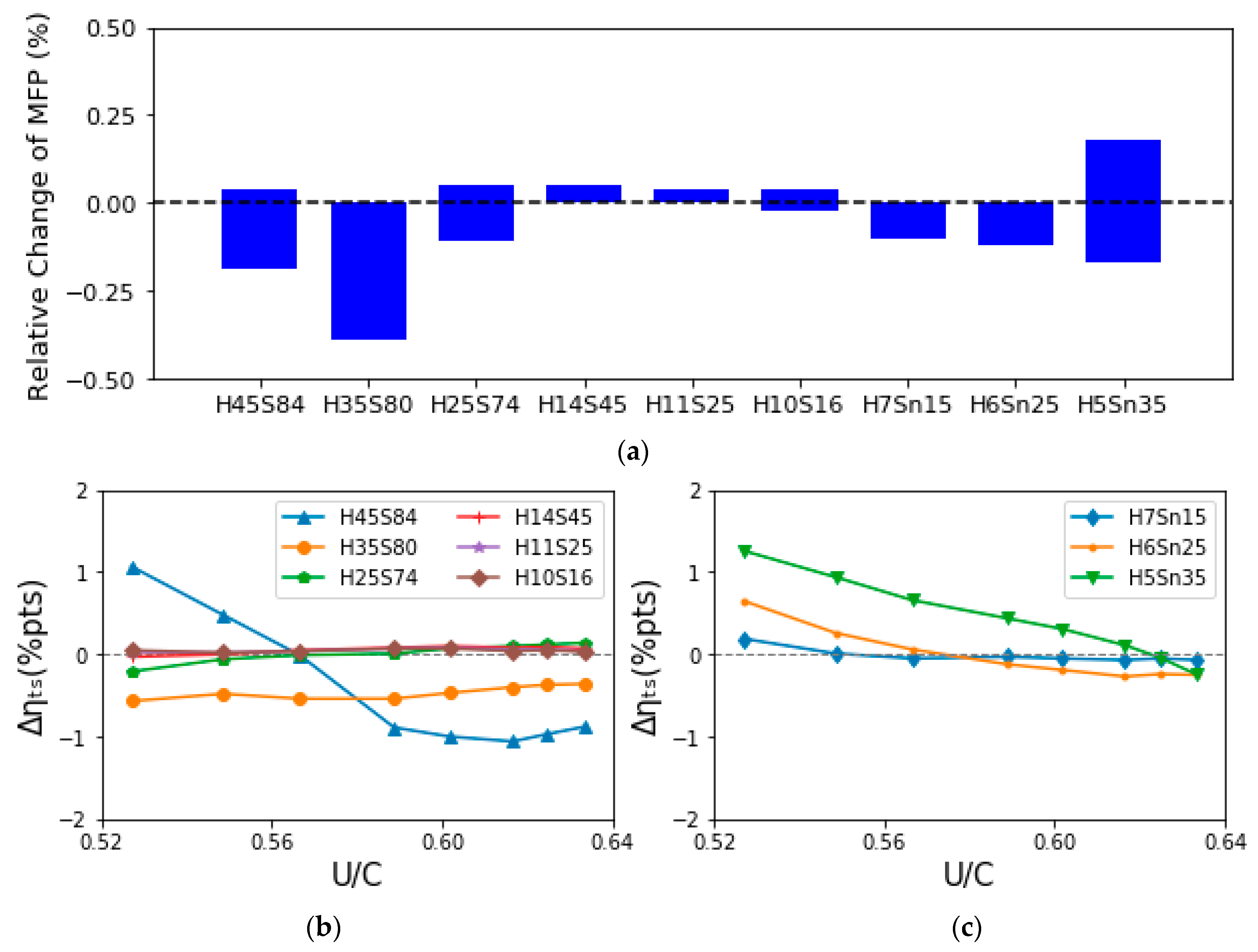
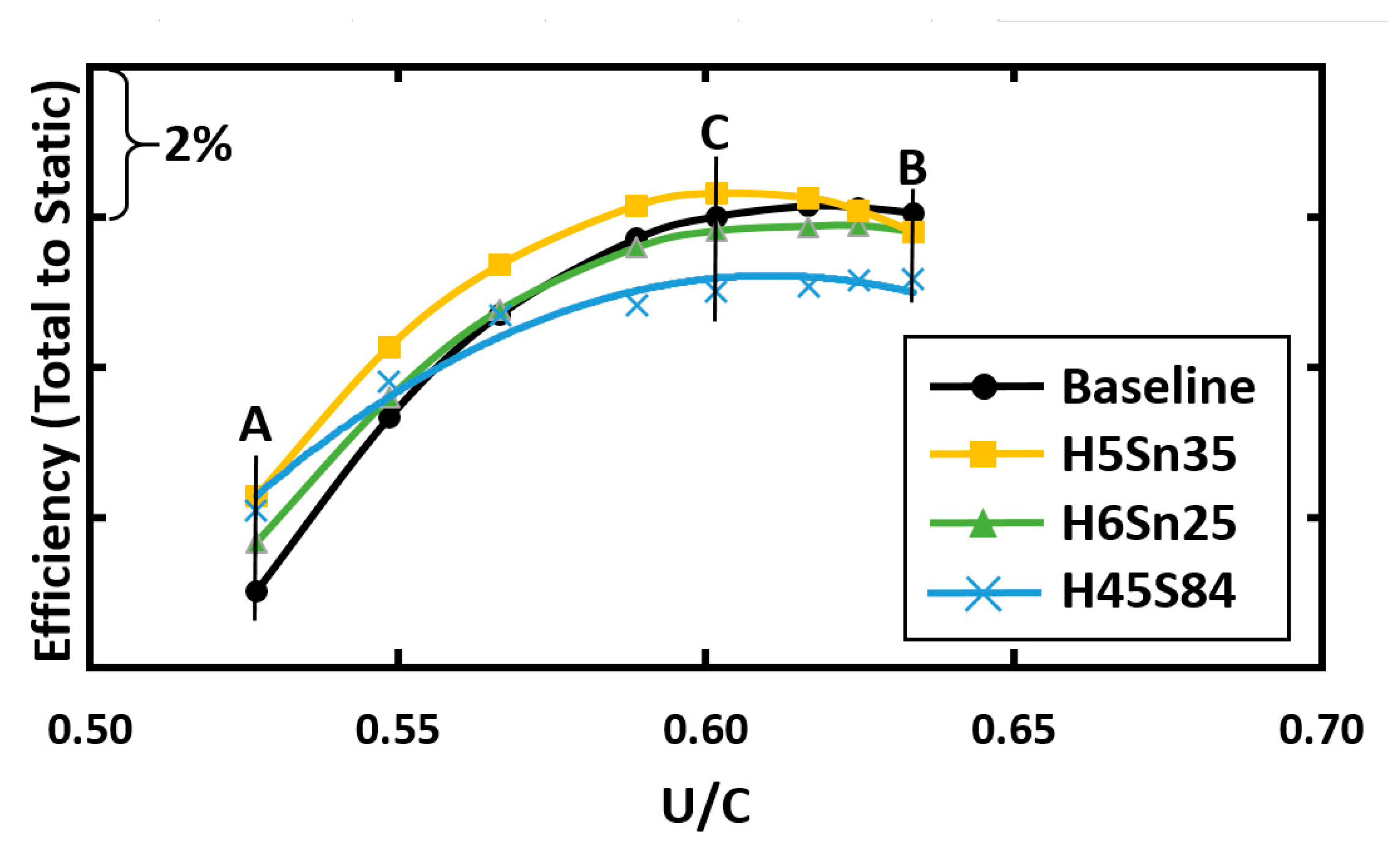
3.1. General Performance

The general performance of all stator tilting endwall designs at the design speed are presented in Figure 7. As a direct comparison to the baseline, the relative change of MFP and efficiency are shown instead of its absolute value. In terms of MFP, the relative change was calculated for each working point on the performance curve. Then the maximum and minimum value formed the variation range of the bar in Figure 7a. For all the designs, the change of MFP varied between –0.4% and +0.2%. As suggested by [23], the mass flow rates were considered matched if the deviation varied between −0.7% and +0.6% and by only achieving this can different designs be compared directly.
In terms of efficiency, the relative changes are presented across the whole performance curve. The designs were categorized into two groups: designs with positive δs (Figure 7b) and designs with negative δs (Figure 7c). In Figure 7b, the tilting endwall had a minor effect on the performance except for design H35S80 and H45S84. For H35S80, the efficiency values on the whole curve were below the baseline. Design H45S84 had even lower efficiency on the high U/C side than H35S80. The relative efficiency change reached the lowest value, i.e., −1.1% points(pts) at U/C =0.62. But as U/C decreased from 0.57, the relative change of efficiency increased to +1.1% pts at the low U/C end. In Figure 7c, all three designs with negative δs achieved higher efficiency on the low U/C side. The efficiency gain increased as δs became more negative from −15° to −35°. The highest efficiency gain was +1.3% pts for design H5Sn35. As U/C rose, for H7Sn15 and H6Sn25, the efficiency gain disappeared at U/C = 0.58, while the efficiency gain of design H5Sn35 remained until U/C = 0.62. At the high U/C end, there was no monotonic relationship between the efficiency and the δs. Specifically, both H5Sn35 and H6Sn25 had more efficiency loss (−0.25% pts) than H7Sn15 (−0.1% pts). In a cross-comparison between Figure 7b,c, even though H45S84 and H5Sn35 both achieved noticeable efficiency gain on the low U/C end, the relatively higher efficiency of H5Sn35 on the high U/C side meant that it gave the best overall performance in this comparison.
Design H5Sn35 had a promising efficiency gain at the low U/C end of the performance curve. However, due to the significant change of endwall geometry, a mesh independence study was needed. Three mesh configurations were investigated, as shown in Table 1. The standard configuration had the grid density that was used to generate all CFD results throughout this paper. The other two configurations were refined configurations, and the element number was normalized by the standard one. The mesh independence study was conducted on three operating conditions with different U/C values, i.e., the end points of the performance curve and the peak efficiency point of design H5Sn35. A direct view of these operating conditions can be seen in the following contents. It can be seen from Figure 8 that the maximum deviation between the standard and the extra fine configurations is −0.8% for MFP and −0.2% pts for efficiency. Despite the MFP deviation, all three mesh configurations of the H5Sn35 design predicted similar MFP values to the baseline. The difference of MFP fell within the range of −0.7% to +0.6% [23], indicating the two designs were comparable. The negative deviation of efficiency meant the extra fine mesh predicted an even higher efficiency improvement at the low U/C end operating condition. Although the extra fine mesh may predict a more accurate result, its application in the current study was limited by the heavy computational effort it needed. This was especially a key issue when predicting the performance curves and conducting unsteady simulations. Therefore, as a trade-off, the standard configuration was still chosen in the following contents.
Since design H5Sn35 achieved the best performance out of the design matrix, a detailed analysis of its flow field was needed to understand the reason for its performance improvement. In addition, since the improvement trend was already evident in design H6Sn25, it was considered useful to compare H5Sn35 with H6Sn25 to understand their differences. The other interesting design was H45S84 which showed a similar level of improvement at the low U/C end as H5Sn35 but a rather low efficiency at the high U/C end. A detailed analysis of its flow field could enhance the understanding of the similarities and differences between H5Sn35 and H45S84. Therefore, three designs, namely H5Sn35, H6Sn25, and H45S84, were selected for detailed flow-field analysis. The efficiency curves of these three designs and the baseline are shown in Figure 9. Compared to the baseline, the peak efficiency point of design H5Sn35 had a distinct shift to the low U/C side, i.e., from 0.62 to 0.60 and the peak efficiency increased by 0.2% pts. Based on the efficiency curve of H5Sn35, three working points were selected for the flow field analysis: the extreme ends of the curve, point A (U/C = 0.53) and B (U/C = 0.63); and the peak efficiency point, point C (U/C = 0.60).

3.2. Analysis at Point A

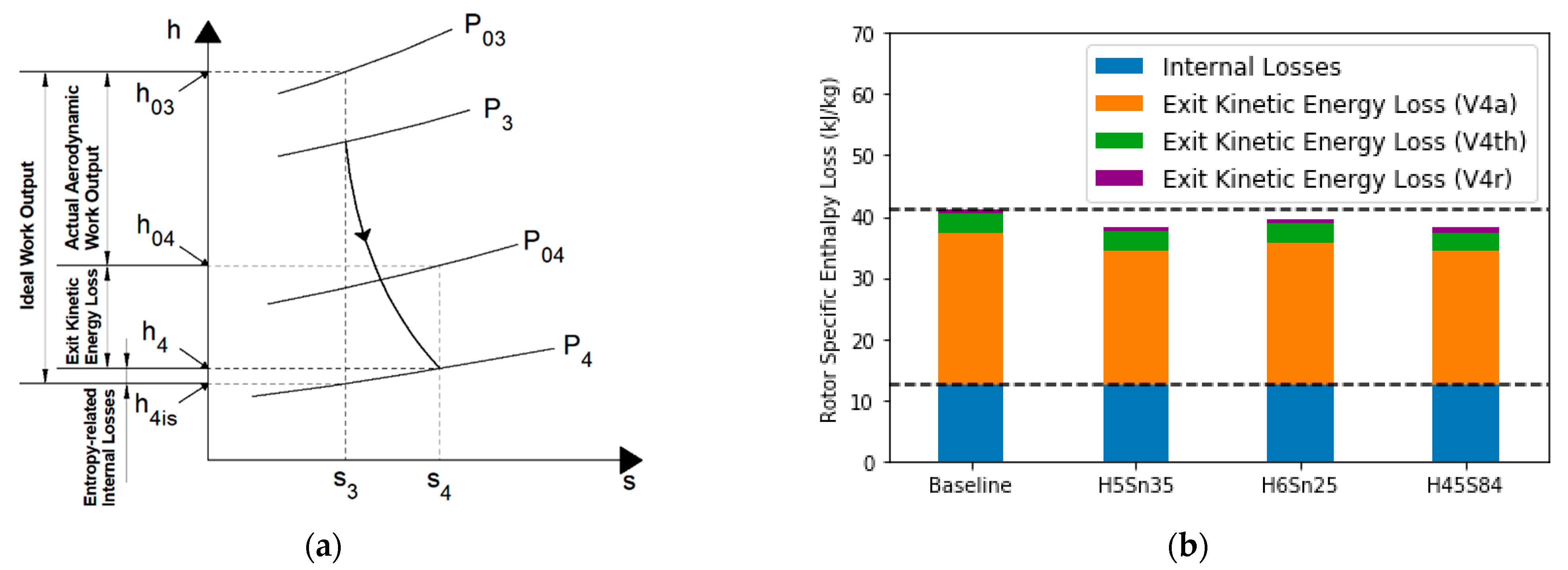
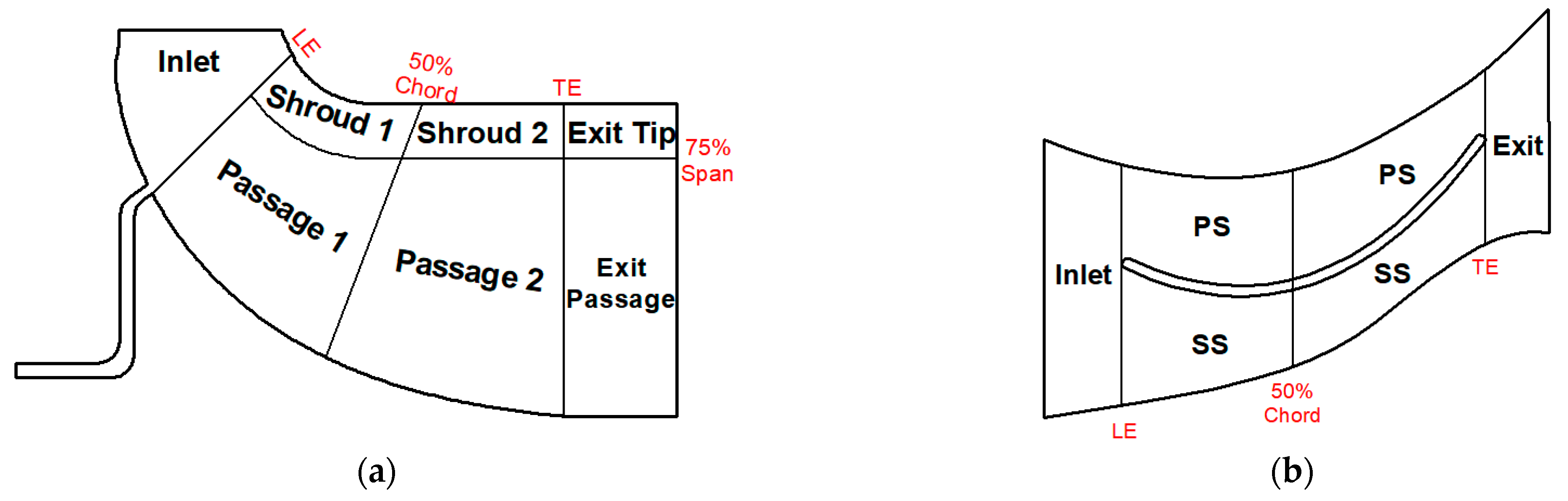
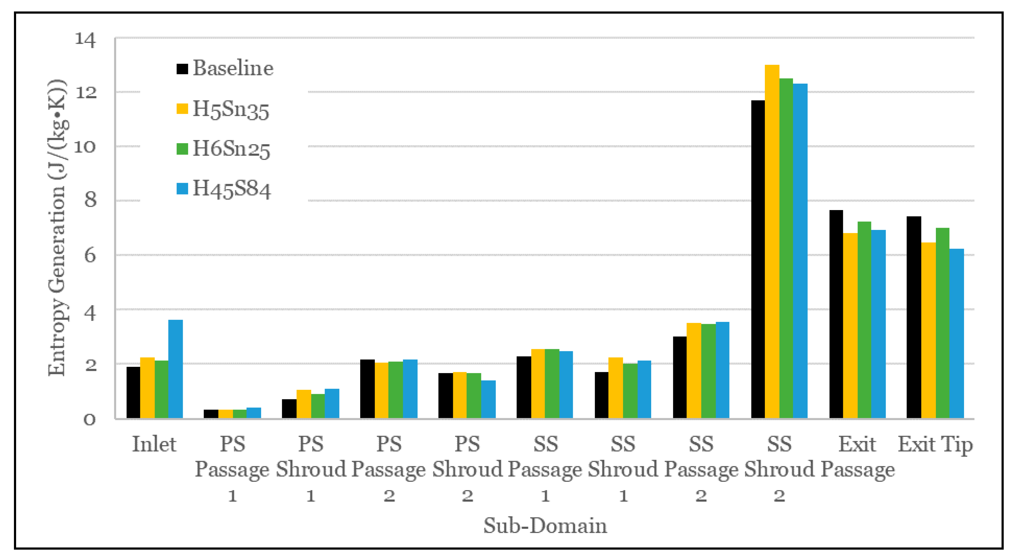
3.2.1. Loss Breakdown

To find out the reason for the performance improvement, the performance was evaluated for each computational domain. Three performance coefficients were selected for the evaluation, namely the total pressure loss coefficient K for the pre-swirl vane and stator domains, the rotor efficiency ηts,rotor and the exhaust diffuser effectiveness εdiffiser, as defined in Equations (3)–(5).
K = P 01 P 02 P 02 P 2   o r   P 02 P 03 P 03 P 3
η t s , r o t o r = 1 ( T 04 / T 03 ) 1 ( P 4 / P 03 ) ( k 1 ) / k
ε d i f f u s e r = ( P 5 P 4 ) ( P 04 P 4 ) ( P 05 P 5 )
Table 2 lists the value of these coefficients for the baseline and the selected designs. In terms of the pre-swirl vane and the stator domain, the K values had almost no change in the first three designs. However, there was an increase of K value in the H45S84 design, which meant higher losses in the pre-swirl and stator domains. For the rotor and the diffuser, the performance coefficients were presented in the form of changes relative to the baseline. It can be seen that all selected designs showed higher rotor efficiency and diffuser effectiveness than the baseline, which were the main reasons for the performance improvement at point A. By comparing H5Sn35 and H45S84, it can be seen that even though the efficiency gains of the rotor domain were almost the same, the stage efficiency of H45S84 was still lower because of the higher losses of the pre-swirl vane and the stator and the relatively lower effectiveness of the diffuser. The higher losses of the pre-swirl vane and the stator were mainly due to the relatively higher flow velocity inside these domains and this higher velocity was caused by the downstream endwall flow separation and the aerodynamic blockage, which is discussed in Section 3.2.2. Since the rotor was one of the main sources for the performance improvement, and the diffuser effectiveness was related to the outflow conditions of the rotor [24], a loss breakdown and flow field analysis will be presented only for the rotor domain.
Figure 10 illustrates the loss breakdown in the rotor for the baseline and the selected designs. In the enthalpy-entropy diagram (Figure 10a), the expansion process in the rotor was represented by the arrowed curve. Four specific enthalpy values (namely h03, h04, h4, h4is) were marked in this diagram which could be used for the loss breakdown. As shown in Figure 10a, the ideal work output could be calculated as an enthalpy difference. Furthermore, this enthalpy difference could be divided into three sections: the actual aerodynamic work output; the exit kinetic energy loss; and the entropy-related internal losses. It should be noted here that exit kinetic energy loss could have a further breakdown by the rotor outlet velocity components:
Δ h 4 , e x i t   k i n e t i c   e n e r g y   l o s s = h 04 h 4 = V 4 2 2 = V 4 a 2 2 + V 4 t h 2 2 + V 4 r 2 2
Among the four entropy values in Figure 10a, only the h4is could not be extracted directly from the CFD results. Instead, it was calculated from the efficiency definition, as presented in Equation (7):
h 4 i s = h 03 ( h 03 h 04 ) η t s , r o t o r
Provided h4is, the specific enthalpy loss could be calculated for each loss component, as shown in Figure 10b. Each bar was stacked by the internal losses (lower) and the exit kinetic energy losses (upper). The exit kinetic energy loss was further divided into the loss of each velocity component using Equation (6). Two dash lines indicate the internal loss and the total loss of the baseline design. It can be seen that in all designs the exit kinetic energy accounted for more loss than the internal losses, which could be due to the high-pressure ratio and the high flow rate at operating point A. In terms of the internal losses, all selected designs actually had slightly higher losses than the baseline. In contrast, a lower total exit kinetic energy loss was seen in all selected designs. This reduction of the total exit kinetic energy loss was the main reason for the rotor efficiency gain. By checking each component of the exit kinetic energy loss, it was found that the loss reduction resulted mainly from the variation of axial velocity (V4a). To find out the reason for the variation, detailed flow field analysis was needed.

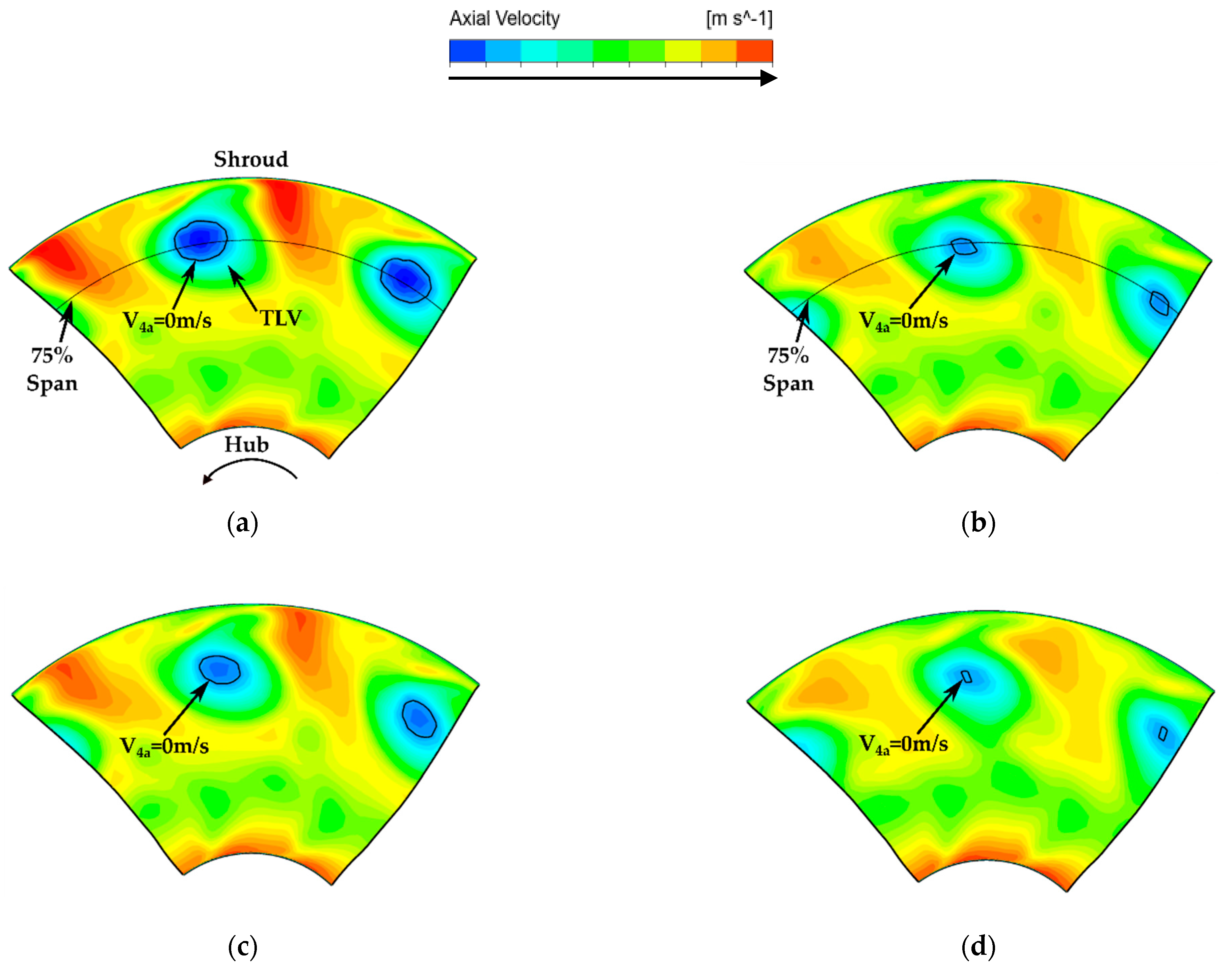
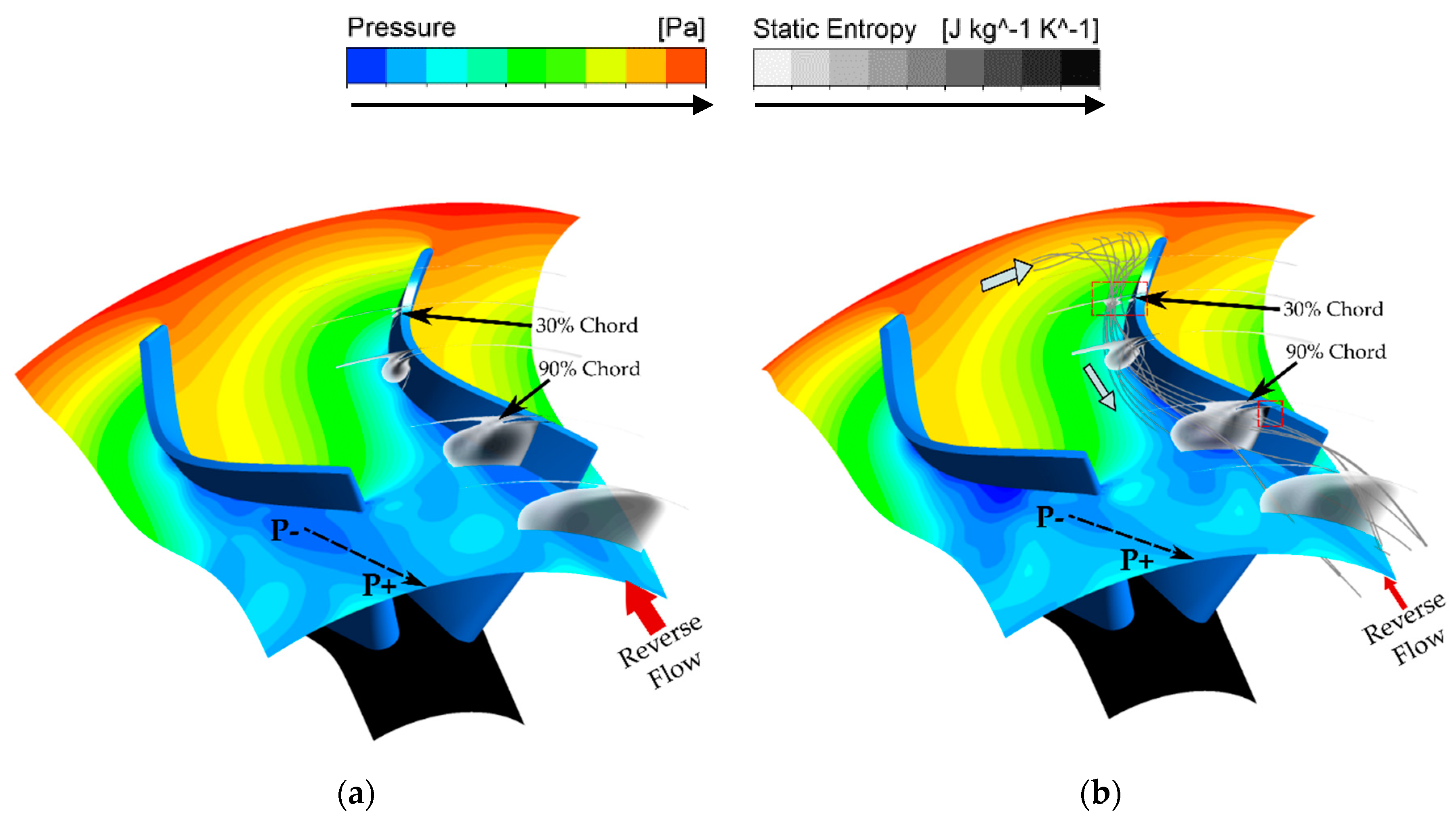
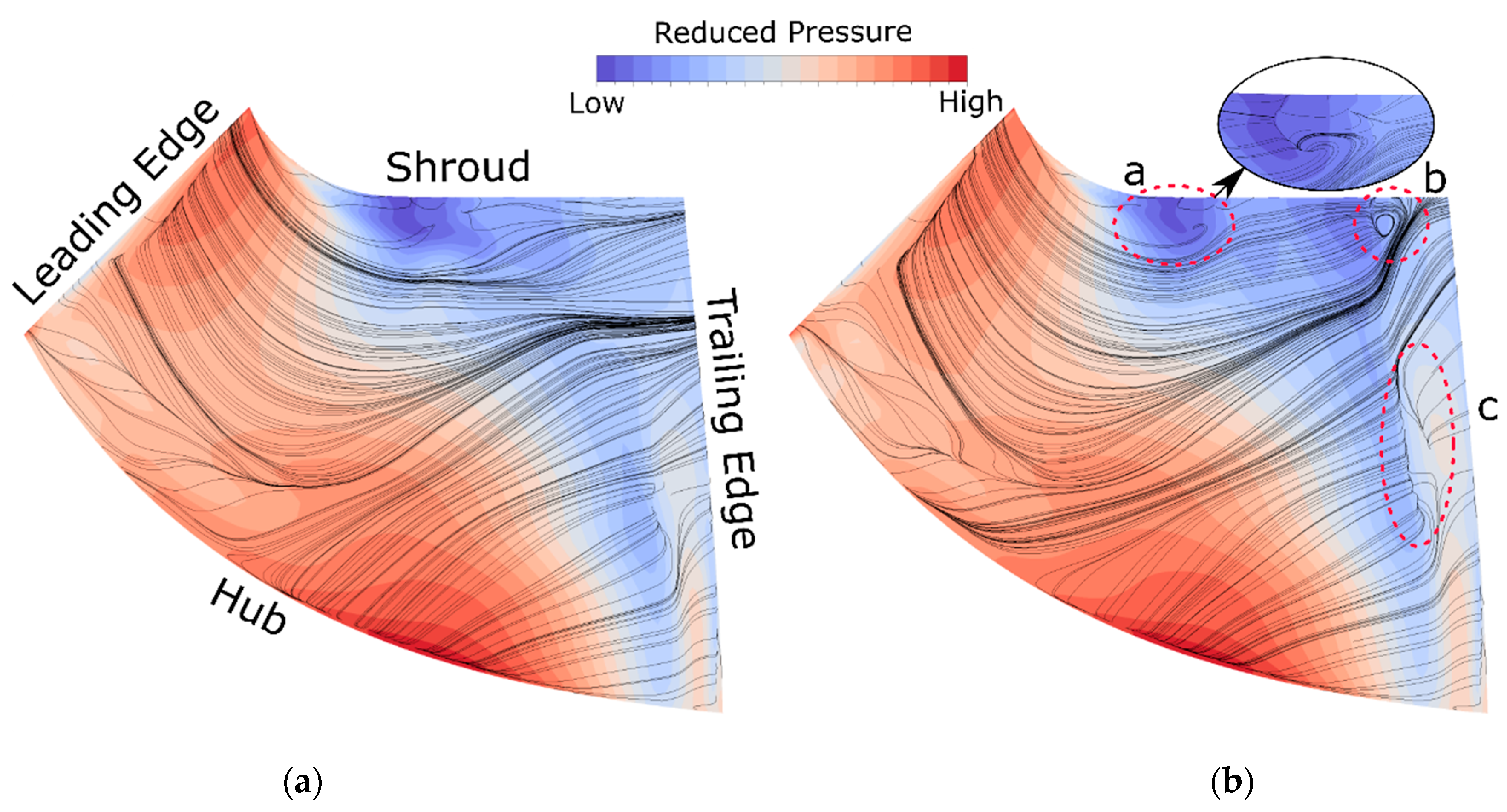
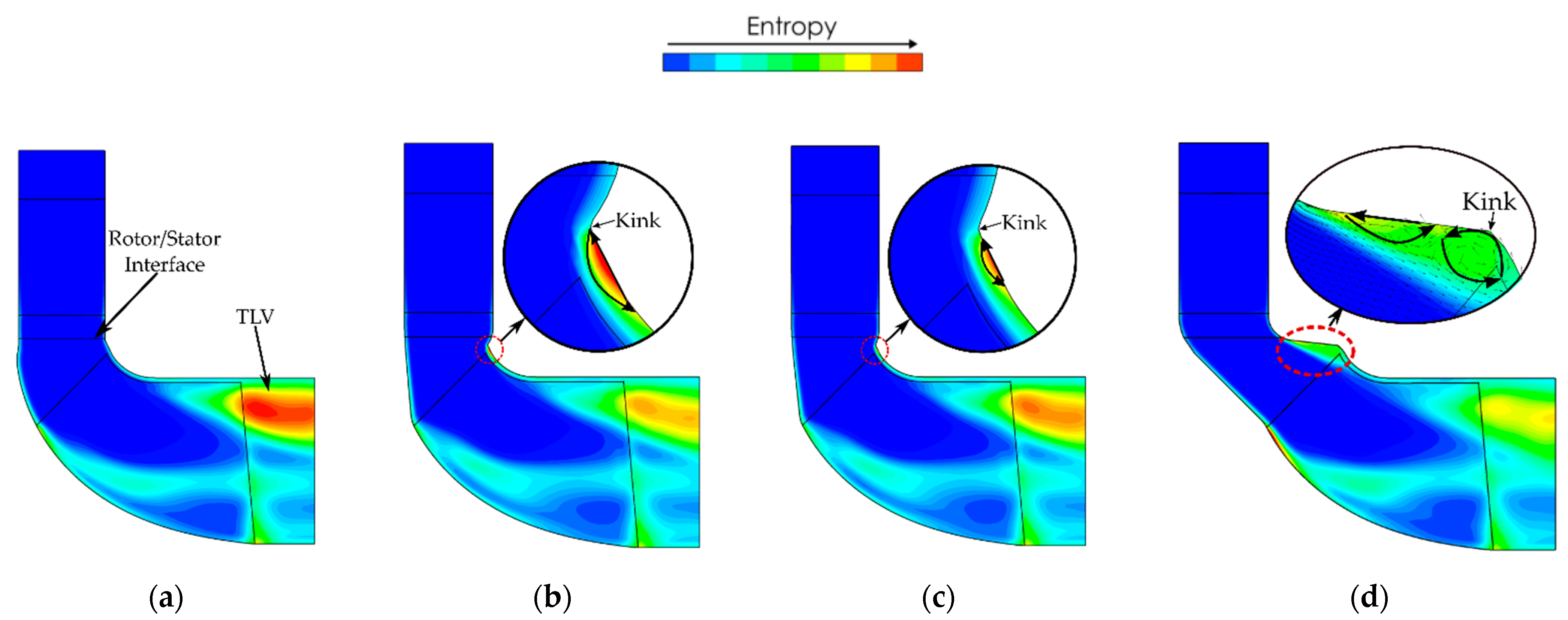
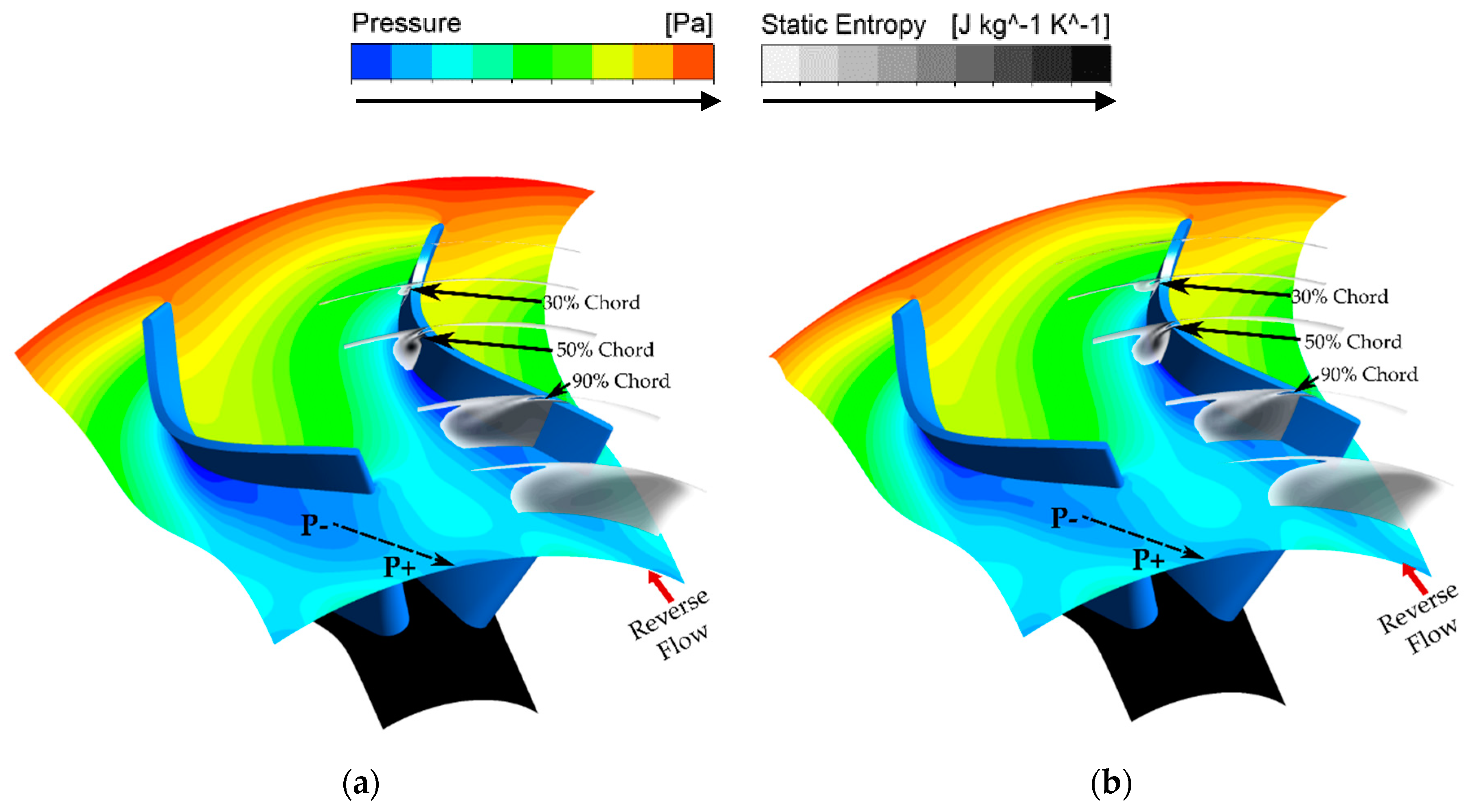
3.2.2. Flow Field Analysis

Figure 11 shows the contour of V4a at the rotor outlet (station 4 in Figure 3b) for the baseline and the three selected designs. For all designs, two rotor passages were presented for a better illustration. As shown, all designs had low V4a regions at the upper half of the outlet. At the center of these regions, the V4a value even became negative implying a reverse flow re-entering into the rotor domain. These low V4a regions were mainly due to the interaction of TLV and low momentum secondary flows that accumulated at the shroud suction corner of the blade passage [25]. As the interacted flow left the blade passage, it moved together with the main flow and reached station 4. As an MFT, the TLV might be the dominant flow feature due to its high blade loading on the shroud side [26]. Therefore, the name “TLV” was used to represent the interacted flow in the following discussions. Adjacent to the low V4a region, there were regions of high V4a near the shroud. These high V4a regions were due to the mid-passage flow which had not been affected by the TLV. Due to the blockage effect of the TLV, the mid-passage flow reached a higher V4a to enable the mass flow pass through. This pattern of V4a near the shroud was in broad agreement with the measurement results of [27], despite the reverse flow which might be caused by the existence of the exhaust diffuser in this study. A comparison between Figure 11a,d showed a relatively stronger contrast of V4a distribution in the baseline (Figure 11a). This distribution in Figure 11a equated to a greater non-uniformity of the flow field at the diffuser inlet for the baseline case. Meanwhile, Figure 11b–d presented a relatively smaller difference between the high and low V4a regions, corresponding to a more uniform flow field at the diffuser inlet than for the baseline. According to [24], improved uniformity of the inlet flow can be expected to enhance the effectiveness of the exhaust diffuser.
To give a further insight to the V4a distribution, the static pressure distribution on the 75% span surface of the rotor is shown in Figure 12 for the baseline and the H5Sn35 design. The 75% span was selected because it cut through the center of the low axial velocity regions that were identified in Figure 11a,b. The static pressure contours in Figure 12 present low pressure regions at the rear part of the blade suction surface for both designs. From that low pressure region to the rotor domain outlet, the flow encountered an adverse pressure gradient (as shown by the dashed arrow lines). It was this adverse pressure gradient that caused the reverse flow at the rotor domain outlet. One possible reason for the adverse pressure gradient was the diffusing flow resulting from the suction surface curvature. Another reason was the development of the TLV and its detachment from the blade surface. The development of the TLV could be seen from the high static entropy regions on selected streamwise sections, which are shown as the grayscale contours in Figure 12. As the TLV developed in the streamwise direction, the extent of the high entropy region increased and from a certain streamwise point the TLV started to intersect with the 75% span surface. The high entropy regions caused by the TLV also had low pressure values due to its high losses. It can be seen in Figure 12 that the high entropy regions of the 90% chord section propagated in the same direction as the adverse pressure gradient. By comparing the two designs, it can be seen that the H5Sn35 case had lower entropy values in the TLV region, e.g., at the 90% chord section, which corresponded to less loss and higher static pressure in the TLV region of this design. As a result, the adverse pressure gradient was reduced in H5Sn35 and thus there was a reduction of the low V4a region, which explained the difference of the V4a distribution in Figure 11a,b.
By checking Figure 12b, it was found that at 30% chord section there was an additional high entropy region (marked by a red rectangle) next to the TLV in design H5Sn35. By plotting the streamlines through this region, it was found that this region resulted from the separated flow induced by the geometric kink of the stator endwall (see Figure 6i). Because of the pressure difference between the blade pressure and suction side, the separated flow first migrated to the suction side near the blade leading edge and then entered into the rotor passage. In the downstream region, this separated flow mixed and rotated together with the TLV. Since the separated flow had low momentum, its mixing with the TLV reduced the intensity of the TLV and thus the entropy generation of the TLV. A similar description could be found in [26] which investigated an RFT with sharp turning on the shroud endwall.
Since the high entropy region at the shroud suction corner could be affected by the low momentum secondary flow on the blade suction surface [25], the secondary flow on the suction surface was analyzed by plotting the skin friction lines for the baseline and the H5Sn35 designs at operating point A, as shown in Figure 13. In addition, the reduced static pressure Pr defined as Equation (8) was also plotted as contours in the same figure. Although the concept of Pr is borrowed from incompressible flows, it has been used to conceptually explain the direction of movement of the near-wall secondary flow in radial and mixed flow turbines [19,25]. From the skin friction lines, separated flow regions were found in both designs (marked as “a”) near the middle-chord of the shroud. The separation was due to the convex turning of the blade and the high blade loading at that region. However, there were two main differences between designs, which were marked as “b” and “c.” At region “b,” an additional separated flow was seen only in H5Sn35 design, which corresponded to the local high entropy region at 90% chord in Figure 12b (marked by a red rectangle). At region “c,” the separated flow region in H5Sn35 was larger than the baseline, which was caused by the intensified local adverse gradient of the reduced pressure. The separated flows in these two regions contributed to the slightly higher internal losses in H5Sn35. By examining the Pr contours, a distinct difference was seen as the low Pr region right before region “b” in Figure 13b. As can be seen from the streamline, this low Pr region formed before the up-moving secondary flow affected the shroud trailing edge region. Therefore, it was believed that the low Pr region was mainly attributed to the interaction of vortices near the shroud region instead of the up-moving secondary flow on the suction surface of the blade.
P r = P 0.5 ρ ω 2 r 2
Figure 14 further illustrates the relationship between the TLV and the separated flow caused by the endwall kink. For all the designs in Figure 14, there were generally two high entropy regions: one near the hub side of the middle chord of the blade and one near the shroud side of the outlet. The high entropy region near the hub was due to the hub corner separation on the suction side of the blade surface and the vortex from the back-disk cavity. For all the designs in Figure 14, there were no distinct differences for the entropy generation in this region. The high entropy regions near the shroud were mainly due to the TLV and they correlated to the high entropy and the low pressure region in Figure 12. For all the selected designs, namely Figure 14b–d, separated flows caused by the endwall kink can be seen from the enlarged views. It was these separated flows that reduced the entropy generated by the TLV near the shroud-outlet region. By comparing Figure 14b,c, it was found that the kink-induced separated flow in Figure 14b generated higher entropy due to the more drastic turning of the shroud endwall. The higher entropy indicated a lower momentum of the separated flow which led to the better performance by reducing the TLV intensity. Therefore, design H5Sn35 outperformed H6Sn25 in that sense. Design H45S84 also had a separation region on the shroud side before the leading edge, which can generate low-momentum flows and thus reducing the TLV intensity. However, different from the other two designs, the separation in H45S84 happened upstream of the kink. The separated flow was actually caused by the shroud “kink-like” endwall profile near the rotor/stator interface.
There was a clear reduction of the entropy generated by the TLV in Figure 14b,d compared with the baseline (Figure 14a). It meant the internal losses caused by the TLV were reduced near the shroud-outlet region. However, as presented in Figure 10b, the overall internal enthalpy losses in the rotor domain showed no distinct change between these designs. This was mainly due to the increase of losses in other regions of the rotor. To quantify the change of internal losses in different regions of the rotor, the rotor was divided into 11 sub-domains, as shown in Figure 15. As suggested by [28], the entropy generation was a reliable method to measure the internal losses. In [19], the entropy generation of each sub-domain was calculated using Equation (9):
s u b d o m a i n ρ D s D t d V = s u r f a c e s d m ˙
The left-hand side is the entropy generation obtained by a volume integration of the entropy generation rate. With the adiabatic and steady-state assumption, the entropy generation equated to the net entropy flux through the sub-domain surfaces, which was presented on the right-hand side. Apart from this entropy flux method, the entropy generation can also be calculated directly from the dissipation and temperature gradient, e.g., [29]. However, the entropy flux method is argued to be a relatively simpler method for 3D fluid model [30] and application examples on MFTs can be found in [12,19,31]. As a result, the entropy flux method was selected in this study for the loss analysis.
The entropy generation in each sub-domain is presented in Figure 16. In the Exit Tip and Exit Passage sub-domains, less entropy was generated for the selected designs than in the baseline, which was consistent with the entropy contour in Figure 14. However, more entropy generation was observed in almost all other sub-domains. In Inlet, PS Shroud 1 and SS Shroud 1 sub-domains, the higher entropy generation values were mainly due to the kink-induced separated flow. This increase of entropy generation was especially evident for design H45S84 in the Inlet sub-domain, which revealed the adverse effect of its complex separated flow as shown in Figure 14d. Another distinct difference was observed in the SS Shroud 2 sub-domain. Although the entropy value of the TLV was lower in this region for the three selected designs, e.g., at the 90% chord section in Figure 12b, the entropy generation value in this domain was actually higher than that for the baseline. The extra entropy was partially generated in other parts of the flow instead of the TLV. One example was the local separated flow on the suction surface near the blade rear-tip region (region ‘b’ in Figure 13b). It caused a locally high entropy value, which was marked by the red rectangle at the 90% chord section in Figure 12b. This extra entropy offset the reduction of entropy in the TLV and thus contributed to a higher overall entropy generation value in the SS Shroud 2 sub-domain.
In summary, the stator tilting endwall designs had three effects: (1) Reducing the TLV intensity and thus the exit kinetic energy losses at the rotor outlet; (2) improving the performance of the exhaust diffuser; (3) but one drawback—introducing additional endwall and other internal losses. The stage performance was dependent upon the combination of all these effects. As can be seen in the Section 3.3, the intensity of these effects might vary as the operating condition changed. Therefore, the net outcome of these effect may not always lead to an improvement of the overall turbine performance.

3.3. Analysis of Points B and C

The main purpose for analyzing point B was to find the reason why design H5Sn35 had lower efficiency than the baseline at this point. The performance coefficient and the rotor loss breakdown are presented in Table 3 for the baseline and H5Sn35. The main performance deficiency of H5Sn35 resulted from the rotor. A loss breakdown of the rotor showed that both the exit kinetic energy loss and the internal losses contributed to the deficiency of design H5Sn35. Similar to the previous case, the axial velocity was the main source causing the difference in the exit kinetic energy loss in the two designs. In addition, there was a minor deterioration of the diffuser effectiveness for design H5Sn35, which resulted from the change of the rotor outlet flow field.
The detailed flow fields for these two designs are presented in Figure 17. The variable range of Figure 17 was different from Figure 12 for a better illustration at this operating point. There were several differences from the flow field in Figure 12, which explained the performance deficiency of design H5Sn35 at point B. First, at the 30% chord section in Figure 17b, there is only one high entropy region near the suction-tip region. It meant the separated flow caused by the endwall kink had already mixed with the TLV at this section, which did not happen for operating point A in Figure 12b. This might be due to the different incidence conditions as the stage pressure ratio changed from point A to point B. Although this early mixing reduced the extreme entropy value of the TLV at the 50% chord section, its effect on the 90% chord and on even further downstream sections could hardly be distinguished. Second, in Figure 17a, the pressure gradient at the rear part of the blade suction surface showed a clear diffusion flow pattern caused by the blade surface curvature. It meant the effect of the TLV on the pressure distribution was not as dominant as at point A. Meanwhile, the additional internal losses caused by the kink-induced separation flow still existed. As a result, design H5Sn35 had lower efficiency than the baseline at point B.
Table 4 presents the performance coefficient and the rotor loss breakdown for the baseline and two selected designs at operating point C. H5Sn35 had the peak stage efficiency at this point. From Table 4 it can be seen that this efficiency improvement was mainly due to the performance improvement of the rotor. Meanwhile, the effectiveness of the diffuser decreased for the tilted stator designs because of the variation of the incoming flow field. By breaking down the rotor losses into the exit kinetic energy loss and the internal loss, it was found that performance improvement resulted mainly from the reduction of exit kinetic energy. It meant the design H5Sn35 at point C had the same mechanism to improve the stage performance as point A. However, as the operating condition approached point B, the magnitude of the efficiency gain became less than point A. In contrast, the efficiency of design H45S84 was 1.25% points lower than the baseline. According to the rotor loss breakdown, both the exit kinetic energy loss and the internal losses contributed to the deficiency. This was mainly due to the excessive flow separation before the rotor leading edge in design H45S84. It added endwall losses to the internal losses. In addition, as a low pressure flow, the kink-induced separated flow together with the TLV intensified the reverse flow at the rotor outlet and thus increased the exit kinetic energy loss.

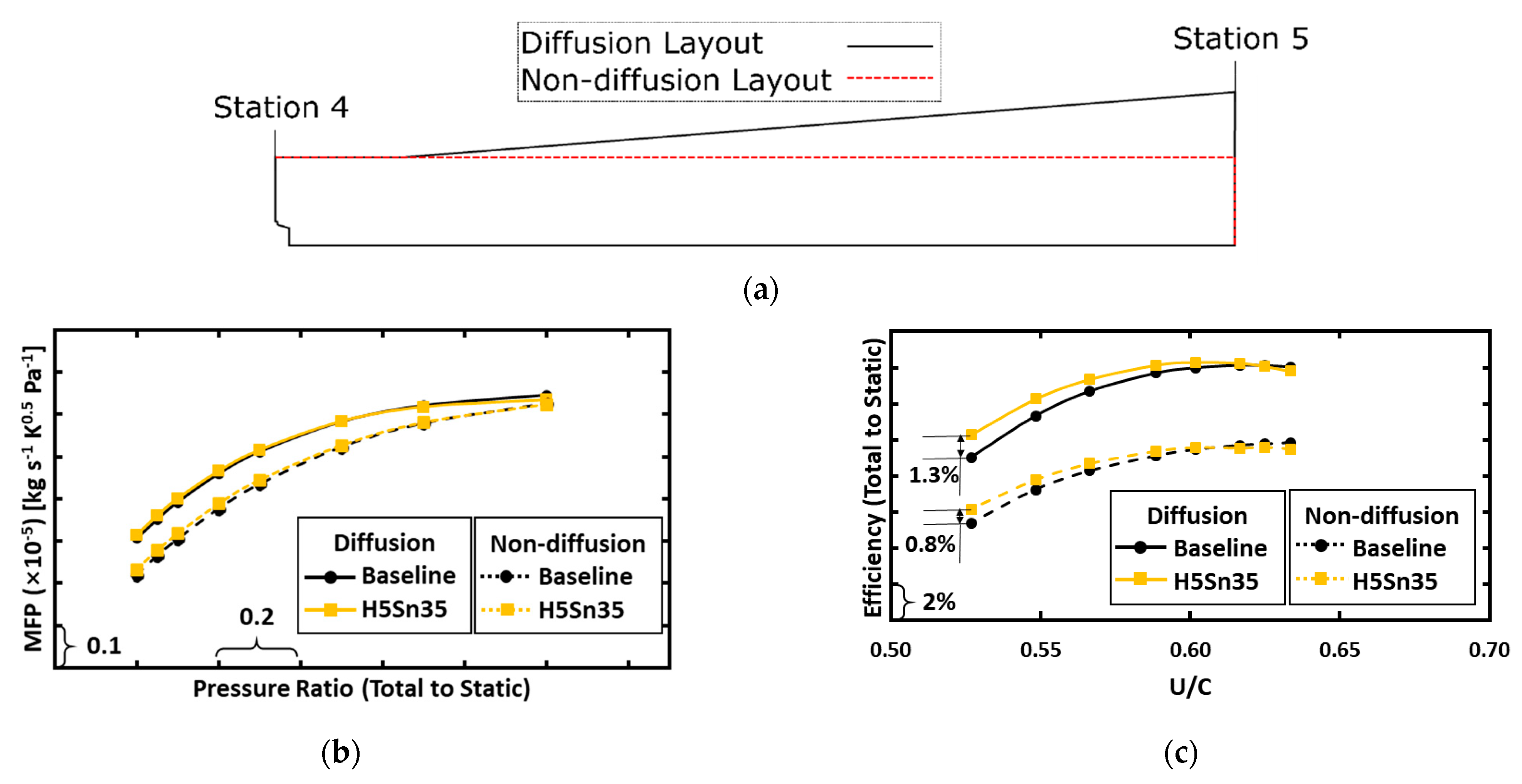
3.4. Preliminary Results without an Exhaust Diffuser

As discussed above, the performance change of the tilted stator designs resulted from both the rotor and the exhaust diffuser. However, some turbocharger installations might not be able to include an exhaust diffuser or at least not as sizeable as the one in this study. To evaluate the performance of the stator tilting endwall designs in such installations, the exhaust diffuser was modified by replacing the divergence shroud with a constant-radius annular one (see Figure 18a). These two layouts were named as “Diffusion” and “Non-diffusion” separately. By connecting the “Non-diffusion” layout with the rotor and other upstream domains shown in Figure 3b, the performance of the turbine stage without an exhaust diffuser could be evaluated. For the “Non-diffusion” layout, both the baseline stator design and the H5Sn35 design were examined and their performance curves were plotted in Figure 18b,c together with the results of the “Diffusion” layout.
In Figure 18b, the MFP curves of the H5Sn35 and baseline stator designs with the “Non-diffusion” layout closely overlapped with each other, which indicated that there was no significant shift of the mass flow. Therefore, the performance of different stator designs was still comparable without the exhaust diffuser. But in general, the “Diffusion” layout had a higher MFP than the “Non-diffusion” layout on the whole performance curve due to the diffusion effect of the exhaust diffuser. This effect caused a higher pressure ratio between the rotor inlet and outlet and thus a higher MFP for the “Diffusion” layout compared with the “Non-diffusion” counterpart.
In Figure 18c, an efficiency gain at the low U/C end was observed for the design H5Sn35 with either the “Diffusion” or the “Non-diffusion” layout. However, this efficiency gain was only 0.8% for the “Non-diffusion” layout, which was relatively lower than the aforementioned 1.3% improvement of the “Diffusion” counterpart. This change was mainly due to two reasons. First, at the low U/C end, the effectiveness of the exhaust diffusor was improved for the H5Sn35 stator design providing additional gain to the stage efficiency (see Table 2). In contrast, the “Non-diffusion” layout lost this part of the efficiency gain due to the lack of exhaust diffuser. Second, for both the “Diffusion” and the “Non-diffusion” layout, the efficiency gain increased toward the low U/C end. Since the efficiency gain resulted mainly from the rotor, it meant a higher pressure ratio between the rotor inlet and outlet might lead to even greater efficiency gain in the rotor. As discussed above, the diffusion effect in the “Diffusion” layout could lead to a higher pressure ratio between the rotor inlet and outlet than the “Non-diffusion” layout. Therefore, this shift of the rotor pressure ratio was another reason for the lower efficiency gain of the “Non-diffusion” layout. However, it should still be noted that the above results showed the capability of the stator tilting endwall design to achieve better performance at the low U/C working conditions and this efficiency benefit increased as the U/C decreased.

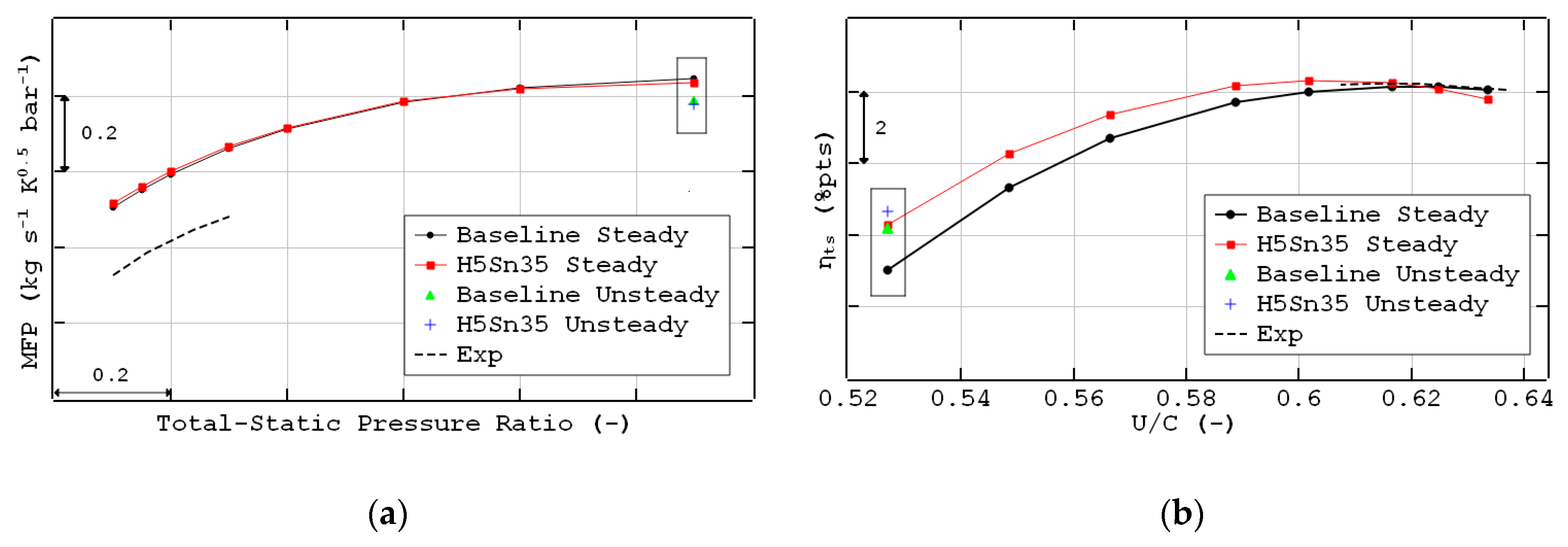
3.5. Preliminary Results of Unsteady CFD Simulations

Unsteady CFD simulations were conducted at operating point A for the baseline and the H5Sn35 designs. The time-transformation method in CFX was utilized to simulate the transient flow between the rotor and the stator domains. To fulfill the requirement of the rotor-stator pitch ratio for the method, the rotor and stator domains were scaled to reach a pitch ratio of 1.09. The other domains were scaled accordingly to maintain a pitch ratio close to 1.0 across the interface. Since the rotor, the cavity and the exhaust diffuser had the same pitch value, the profile-transformation method in CFX was used on the interfaces between them. The inlet and outlet boundary conditions were remained the same as the steady state simulations. The time step was set equal to the time that the rotor needed to rotate 1° about its axis. Two revolutions were set as the total simulation period. In each time step, the simulation was considered to be converged as all RMS residuals reached below 1 × 10⁻⁴ within ten iterations. In the second revolution, the flow parameters at monitored points showed clear periodicity.
The time-averaged unsteady CFD results were plotted together with the steady-state CFD results and the Exp data in Figure 19. The operating point A is marked in a rectangular symbol. In Figure 19a, the MFP predicted by the unsteady CFD simulations were about 1% lower than the steady state results for both designs. But considering the deviation of MFP between the steady state CFD results and the Exp data, the lower MFP predicted by the unsteady simulations may lead to an improved matching with the Exp data. In Figure 19b, the efficiency gain still exists for the unsteady CFD results. However, the improvement reduced from 1.3% pts to 0.5% pts. A detailed analysis of the unsteady CFD simulations is needed in the future to explain the change. Full-360 CFD simulations or Exp data of H3Sn45 may be needed to provide further validation.

4. Conclusions

The numerical study in this paper investigated a series of stator tilting endwall designs in a mixed flow turbine. The numerical method was validated against the experimental data from a cold turbine test facility for the baseline design. By systematically varying the endwall tilting angles, nine stator tilting endwall designs were formed in the design matrix which covered a wide range of tilting angles. The performance of these designs was compared with the baseline at the design speed.
It was found that only the designs at the extremes of the design matrix could present noticeable performance gains compared to the baseline. For most of these extreme designs, the performance gain was only achievable on the low velocity ratio side of the operating range. Only the case with the most negative tilting angle on the shroud side, namely H5Sn35, showed performance improvement across most operating points of the performance curve. Indeed, the efficiency characteristic of design H5Sn35 shifted toward the low velocity ratio side. Its maximum efficiency gain was 1.3% which was achieved at the lowest velocity ratio end of the curve. In addition, the peak efficiency of the H5Sn35 case increased slightly by 0.2% and the corresponding velocity ratio shifted from the 0.62 for the baseline to 0.60. Such improvement in the efficiency characteristic may achieve higher cycle efficiency in a pulsating turbocharger application.
The implementation of the stator tilting endwall formed a kink on the stator shroud endwall. This kink structure generated a local separation bubble before the rotor leading edge. Then the low-momentum separated flow entered into the rotor domain and mixed with the tip leakage vortex. This had three impacts: (1) Reducing the TLV intensity and thus the exit kinetic energy losses at the rotor outlet; (2) improving the performance of the exhaust diffuser; (3) introducing addition endwall and other internal losses. At the low velocity ratio conditions, the beneficial impact on the TLV was dominant and achieved an overall efficiency gain. However, at the high velocity ratio side, the negative effect of additional internal losses tended to dominate and the efficiency deteriorated.
It was found that the intensity of the kink-induced separated flow at rotor inlet was a key design factor. A separated flow that was either too weak (i.e., design H6Sn25) or too strong (i.e., design H45S84) can undermine the stage performance. This intensity was related to the endwall tilting angle and the kink structure. In addition to the performance improvement in this paper, a future study on the design of the kink structure may achieve further efficiency gain.
The stage performance was also considered for turbine stages without an exhaust diffuser. It was found that the stator tilting endwall designs could still achieve efficiency gain at the low velocity ratio side and a shift of the performance curve toward the low velocity ratio side was also observed. The efficiency of the H5Sn35 case was 0.8% higher than the baseline at the low velocity ratio end of the performance curve. The efficiency gain was lower than for the case with an exhaust diffuser. This was because the rotor was working under different outlet static pressures and the exhaust diffuser brought additional performance gain for the tilted stator designs.
The preliminary unsteady CFD results showed a reduced efficiency gain at the low velocity ratio end of the performance curve. The efficiency gain changed from 1.3% points to 0.5% points for the optimal design in this study. A further study based on the full-360 unsteady simulation may be needed in the future. In addition, a direct experimental validation of the tilted stator designs could also be beneficial. In such experiments, both the general performance and the velocity distribution at the rotor outlet should be measured as a way to evaluate the change of kinetic energy at the rotor outlet.
Overall, the results showed that design of the stator endwalls, particularly the endwall angle and the inclusion of a kink before rotor inlet, could produce efficiency benefits at both low velocity ratio conditions and at the peak efficiency point. Therefore, this is an important feature for consideration in the design of mixed flow turbines.

Author Contributions

Conceptualization, Y.G.; methodology, Y.G. and R.M.; software, Y.G. and R.M.; validation, Y.G. and R.M.; formal analysis, Y.G.; investigation, Y.G.; resources, R.M., S.S. and P.R.; data curation, Y.G.; writing—original draft preparation, Y.G.; writing—review and editing, J.F., S.S., R.M. and P.R.; visualization, Y.G.; supervision, J.F. and S.S.; project administration, J.F.; funding acquisition, J.F. and Y.G. All authors have read and agreed to the published version of the manuscript.

Funding

This research received no external funding. The APC was funded by the library of KTH Royal Institute of Technology, Sweden.

Data Availability Statement

No new data were created or analyzed in this study. Data sharing is not applicable to this article.

Acknowledgments

Yang Gao would like to give his special thanks to China Scholarship Council for the scholarship support to his study. The author would also thank KIC InnoEnergy School for their support to the research collaboration with Queen’s University Belfast. Special thanks are also given to ANSYS Inc. and NUMECA for the usage of their software. Part of the computations were enabled by resources provided by the Swedish National Infrastructure for Computing (SNIC) at the PDC Center for High Performance Computing, KTH Royal Institute of Technology, partially funded by the Swedish Research Council through grant agreement no. 2016-07213. The other computations were facilitated by the High Performance Computing (Kelvin) service at Queen’s University Belfast.

Conflicts of Interest

The authors declare no conflict of interest.

Nomenclature

Variables
δstator endwall tilting angle
εdiffuser effectiveness
ηefficiency
ωrotational speed
hspecific enthalpy
Ktotal pressure loss coefficient
kspecific heat ratio
Ppressure
mmass flow
rradius
sspecific entropy
Ttemperature
Urotor tip speed based on mean radius
Vvelocity
Subscripts
0total state
1stage inlet, pre-swirl vane domain inlet
2pre-swirl vane domain outlet, stator domain inlet
3stator domain outlet, rotor domain inlet
4rotor domain outlet, exhaust diffuser domain inlet
5stage outlet, exhaust diffuser domain outlet
aaxial
diffuserexhaust diffuser domain
hhub
indomain inlet
isisentropic
interfacerotor/stator interface
outdomain outlet
preswirlpre-swirl vane domain
rreduced
rotorrotor domain
sshroud
stageturbine stage
statorstator domain
tstotal to static
Abbreviation
CFDcomputational fluid dynamics
CFVcavity flow vortex
EXPexperimental
LEleading edge
MFPmass flow parameter
MFTmixed flow turbine
ptspoints
PSpressure side
QUBQueen’s University Belfast
RFTradial flow turbine
RMSroot-mean-square
SSsuction side
SSTshear stress transport
TLVtip leakage vortex
TEtrailing edge
U/Cblade speed to isentropic jet velocity ratio

References

  1. Leonard, T.; Spence, S.; Starke, A.; Filsinger, D. Numerical and experimental investigation of the impact of mixed flow turbine inlet cone angle and inlet blade angle. J. Turbomach. 2019, 141. [Google Scholar] [CrossRef]
  2. Baines, N.C. Fundamentals of Turbocharging; Concepts NREC: White River Junction, VT, USA, 2005; Volume 1. [Google Scholar]
  3. Baines, N. Radial-and mixed-flow turbine options for high-boost turbochargers. In Proceedings of the 7th International Conference on Turbochargers and Turbocharging, Savoy Palace, London, 14–15 May 2002; pp. 35–44. [Google Scholar]
  4. Fredriksson, C.; Baines, N. The mixed flow forward swept turbine for next generation turbocharged downsized automotive engines. In Proceedings of the ASME Turbo Expo 2010: Power for Land, Sea, and Air, Glasgow, UK, 14–18 June 2010; pp. 559–563. [Google Scholar] [CrossRef]
  5. Chen, H.; Baines, N.C. The aerodynamic loading of radial and mixed-flow turbines. Int. J. Mech. Sci. 1994, 36, 63–79. [Google Scholar] [CrossRef]
  6. Moustapha, H.; Zelesky, M.F.; Baines, N.C.; Japikse, D. Axial and Radial Turbines; Concepts NREC: White River Junction, VT, USA, 2003; Volume 2. [Google Scholar]
  7. Kirtley, K.R.; Beach, T.A.; Rogo, C. Aeroloads and secondary flows in a transonic mixed-flow turbine stage. J. Turbomach. 1993, 115, 590–600. [Google Scholar] [CrossRef]
  8. Chou, C.-C.; Gibbs, C.A. The design and testing of a mixed-flow turbine for turbochargers. SAE Tech. Pap. 1989. [Google Scholar] [CrossRef]
  9. Rajoo, S.; Martinez-Botas, R. Mixed flow turbine research: A review. J. Turbomach. 2008, 130, 044001–044012. [Google Scholar] [CrossRef]
  10. Lee, S.P.; Jupp, M.L.; Nickson, A.K. The introduction of a tilted volute design for operation with a mixed flow turbine for turbocharger applications. In Proceedings of the 2016 7th International Conference on Mechanical and Aerospace Engineering (ICMAE), London, UK, 18–20 July 2016; pp. 165–170. [Google Scholar]
  11. Lee, S.P.; Jupp, M.L.; Nickson, A.K.; Allport, J.M. Analysis of a tilted turbine housing volute design under pulsating inlet conditions. In Proceedings of the ASME Turbo Expo 2017: Turbomachinery Technical Conference and Exposition, Charlotte, NC, USA, 26–30 June 2017. [Google Scholar] [CrossRef]
  12. Lee, S.P.; Barrans, S.M.; Jupp, M.L.; Nickson, A.K. Investigation into the impact of span-wise flow distribution on the performance of a mixed flow turbine. In Proceedings of the ASME Turbo Expo 2018: Turbomachinery Technical Conference and Exposition, Oslo, Norway, 11–15 June 2018. [Google Scholar] [CrossRef]
  13. Morrison, R.; Spence, S.; Kim, S.; Filsinger, D.; Leonard, T. Investigation of the effects of flow conditions at rotor inlet on mixed flow turbine performance for automotive applications. In Proceedings of the International Turbocharging Seminar 2016, Tianjin, China, 21–22 September 2016. [Google Scholar]
  14. Gao, J.; Zheng, Q.; Yue, G. Reduction of tip clearance losses in an unshrouded turbine by rotor casing contouring. J. Propuls. Power 2012, 28, 936–945. [Google Scholar] [CrossRef]
  15. Dambach, R.; Hodson, H.P.; Huntsman, I. 1998 turbomachinery committee best paper award: An experimental study of tip clearance flow in a radial inflow turbine. J. Turbomach. 1999, 121, 644–650. [Google Scholar] [CrossRef]
  16. Leonard, T.M.; Spence, S.; Early, J.; Filsinger, D. A numerical study of inlet geometry for a low inertia mixed flow turbocharger turbine. In Proceedings of the ASME Turbo Expo 2014: Turbine Technical Conference and Exposition, Dusseldorf, Germany, 16–20 June 2014. [Google Scholar] [CrossRef]
  17. Morrison, R.; Spence, S.; Kim, S.I.; Leonard, T.; Starke, A. Evaluating the use of leaned stator vanes to produce a non-uniform flow distribution across the inlet span of a mixed flow turbine rotor. J. Turbomach. 2020, 142. [Google Scholar] [CrossRef]
  18. Deng, Q.; Niu, J.; Mao, J.; Feng, Z. Experimental and numerical investigation on overall performance of a radial inflow turbine for 100kW mircoturbine. In Proceedings of the ASME Turbo Expo 2007: Power for Land, Sea, and Air, Montreal, QB, Canada, 14–17 May 2007; pp. 919–926. [Google Scholar] [CrossRef]
  19. Yang, B.; Newton, P.; Martinez-Botas, R.F. Understanding of secondary flows and losses in radial and mixed flow turbines. J. Turbomach. 2020, 142, 1–29. [Google Scholar] [CrossRef]
  20. Liu, Y.; Yang, C.; Qi, M.; Zhang, H.; Zhao, B. Shock, leakage flow and wake interactions in a radial turbine with variable guide vanes. In Proceedings of the ASME Turbo Expo 2014: Turbine Technical Conference and Exposition, Dusseldorf, Germany, 16–20 June 2014. [Google Scholar]
  21. Palenschat, T.; Newton, P.; Martinez-Botas, R.F.; Müller, M.; Leweux, J. 3-D computational loss analysis of an asymmetric volute twin-scroll turbocharger. In Proceedings of the ASME Turbo Expo 2017: Turbomachinery Technical Conference and Exposition, Charlotte, NC, USA, 26–30 June 2017. [Google Scholar] [CrossRef]
  22. Cao, T.; Xu, L.; Yang, M.; Martinez-Botas, R.F. Radial turbine rotor response to pulsating inlet flows. J. Turbomach. 2013, 136. [Google Scholar] [CrossRef]
  23. Simpson, A.T.; Spence, S.W.T.; Watterson, J.K. Numerical and experimental study of the performance effects of varying vaneless space and vane solidity in radial turbine stators. J. Turbomach. 2013, 135, 031001–031012. [Google Scholar] [CrossRef]
  24. Japikse, D.; Baines, N.C. Introduction to Turbomachinery; Concepts ETI: White River Junction, VT, USA, 1994. [Google Scholar]
  25. Zangeneh-Kazemi, M.; Dawes, W.N.; Hawthorne, W.R. Three dimensional flow in radial-inflow turbines. In Proceedings of the ASME 1988 International Gas Turbine and Aeroengine Congress and Exposition, Amsterdam, The Netherlands, 6–9 June 1989. [Google Scholar]
  26. Palfreyman, D.; Martinez-Botas, R.F. Numerical study of the internal flow field characteristics in mixed flow turbines. In Proceedings of the ASME Turbo Expo 2002: Power for Land, Sea, and Air, Amsterdam, The Netherlands, 3–6 May 2002; pp. 455–472. [Google Scholar] [CrossRef]
  27. Karamanis, N.; Martinez-Botas, R.F.; Su, C.C. Mixed flow turbines: Inlet and exit flow under steady and pulsating conditions. J. Turbomach. 2000, 123, 359–371. [Google Scholar] [CrossRef]
  28. Denton, J.D. The 1993 IGTI scholar lecture: Loss mechanisms in turbomachines. J. Turbomach. 1993, 115, 621–656. [Google Scholar] [CrossRef]
  29. Kock, F.; Herwig, H. Entropy production calculation for turbulent shear flows and their implementation in cfd codes. Int. J. Heat Fluid Flow 2005, 26, 672–680. [Google Scholar] [CrossRef]
  30. Newton, P. An Experimental and Computational Study of Pulsating Flow within a Double Entry Turbine with Different Nozzle Settings. Ph.D. Thesis, Imperial College London, London, UK, 2014. [Google Scholar]
  31. Elliott, M.; Spence, S.; Seiler, M.; Geron, M. Performance improvement of a mixed flow turbine using 3D blading. In Proceedings of the ASME Turbo Expo 2020: Turbomachinery Technical Conference and Exposition, Virtual Conference. 21–25 September 2020. [Google Scholar]
Figure 1. Schematic representations: (a) The pulsating pressure at the turbine inlet and the turbine power output in an engine cycle; (b) a shift of efficiency curve towards low U/C side.
Ijtpp 06 00014 g001
Figure 2. Stator endwall designs for MFT (Volute, stator vanes and other components are not presented; endwalls are elongated for illustration purpose). (a) Perpendicular, (b) tangential, (c) radial.
Ijtpp 06 00014 g002
Figure 3. (a) The MFT rotor model; (b) the meridional view of the baseline stage with the domains, the interfaces and the stations.
Ijtpp 06 00014 g003
Figure 4. Comparison of performance curves between CFD and EXP at the design speed: (a) MFP; (b) efficiency.
Ijtpp 06 00014 g004
Figure 5. (a) Design domain for the stator tilting endwall designs; (b) the baseline and an example design.
Ijtpp 06 00014 g005
Figure 6. Matrix of different stator tilting endwall designs.
Ijtpp 06 00014 g006
Figure 7. Relative performance change for different stator tilting endwall designs: (a) The range of MFP change relative to the baseline; (b) efficiency change relative to the baseline (positive δs designs); (c) efficiency change relative to the baseline (negative δs designs).
Ijtpp 06 00014 g007
Figure 8. Mesh independence study (a) MFP and (b) efficiency comparisons.
Ijtpp 06 00014 g008
Figure 9. Efficiency curves of selected designs for detailed flow field analysis.
Ijtpp 06 00014 g009
Figure 10. (a) Enthalpy–entropy diagram of expansion process in the rotor and (b) loss breakdown of the rotor domain at operating point A (Figure 9).
Ijtpp 06 00014 g010
Figure 11. Axial velocity contour on the surface of station 4 at operating point A (Figure 9). (a) Baseline; (b) H5Sn35; (c) H6Sn25; (d) H45S84.
Ijtpp 06 00014 g011
Figure 12. Pressure distribution on 75% span surface and high entropy regions on streamwise sections at operating point A (Figure 9); (a) Baseline; (b) H5Sn35.
Ijtpp 06 00014 g012
Figure 13. Skin friction lines and reduced pressure contour on rotor blade suction surface at operating point A (Figure 9). (a) Baseline; (b) H5Sn35.
Ijtpp 06 00014 g013
Figure 14. Circumferentially averaged entropy at operating point A (Figure 9). (a) Baseline; (b) H5Sn35; (c) H6Sn25; (d) H45S84.
Ijtpp 06 00014 g014
Figure 15. Schematic views of rotor sub-domains for internal loss analysis. (a) Meridional; (b) blade-to-blade.
Ijtpp 06 00014 g015
Figure 16. Entropy generation of each sub-domain at operating point A (Figure 9).
Ijtpp 06 00014 g016
Figure 17. Pressure distribution on 75% span surface and high entropy regions on streamwise sections at operating point B (Figure 9). (a) Baseline; (b) H5Sn35.
Ijtpp 06 00014 g017
Figure 18. (a) The “Diffusion” and “Non-diffusion” Layouts; (b) MFP curves and (c) efficiency curves of different stator designs with the “Diffusion” and the “Non-diffusion” exhaust Diffusers.
Ijtpp 06 00014 g018
Figure 19. (a) MFP results and (b) efficiency results of steady and unsteady simulations.
Ijtpp 06 00014 g019
Table 1. Element numbers of mesh domains (normalized by the standard configuration).
Mesh ConfigurationPre-Swirl VaneStator VaneRotorCavityDiffuser
Standard11111
Fine1.331.361.361.381.41
Extra Fine1.831.841.821.901.87
Table 2. Performance coefficient of computational domains at point A (Figure 9).
DesignKpre-swirlKstatorΔηts,rotorΔεdiffuser
Baseline0.0390.043--
H5Sn350.0390.042+2.0%+2.2%
H6Sn250.0390.043+1.05%+1.7%
H45S840.0410.047+1.96%+1.8%
Table 3. Performance coefficient of stage components and rotor loss breakdown at operating point B (Figure 9).
DesignKpre-swirlKstatorΔηts,rotorΔhexit kinetic energy (kJ/kg)Δhinternal (kJ/kg)Δεdiffuser
Baseline0.0400.048-12.428.14-
H5Sn350.0400.048−0.3%12.578.26−0.1%
Table 4. Performance coefficient of stage components and rotor loss breakdown at operating point C (Figure 9).
DesignKpre-swirlKstatorΔηts,rotorΔhexit kinetic energy (kJ/kg)Δhinternal (kJ/kg)Δεdiffuser
Baseline0.0400.047-14.749.41-
H5Sn350.0400.045+0.35%14.209.42−0.9%
H45S840.0420.041−1.25%15.759.93−0.4%
Publisher’s Note: MDPI stays neutral with regard to jurisdictional claims in published maps and institutional affiliations.

