1. Introduction
Since the pioneering work of Ainley and Mathieson [
1], several different loss models and loss prediction systems have been developed for steam and gas turbines. Although sophisticated and complex computational fluid dynamics (CFD) methods are widely available, mean line models are still necessary for preliminary axial-flow turbines’ design and optimization. Specific loss models can reasonably predict losses for steam and gas turbines under certain conditions. However, relatively little is known regarding their performance for organic Rankine cycle (ORC) turbines. The impact of the non-perfect gas behavior of the involved organic vapors needs to be addressed in conventional loss systems. The usual practice is to compute perfect gas equivalent input quantities for the loss model as performed, for instance, by Harloff [
2], and the conventional literature loss models or correlations are directly employed. In principle, the careless use of perfect gas quantities for calculating real gas phenomena is not free of fundamental difficulties. Besides the real gas behavior, there is also an additional problem in the experiments with the high molecular weight of the organic fluids and the resulting high-velocity regimes. The literature loss correlations have been established based on the typical Reynolds numbers, roughness levels, and turbulence length scales occurring in steam and gas turbines. Deviations might arise in ORC turbines due to the different ratios between turbulent length scales, roughness, and blade dimensions and their impact on flow separation and boundary layer development.
An inspection of the open literature showed that the conventional loss systems were applied to ORC turbines without any modification or experimental proof of their validity. Macchi and Perdichizzi [
3] presented the results of an efficiency prediction study based on the Craig and Cox [
4] correlation for axial-flow turbines operating with non-conventional fluids. Da Lio et al. [
5] provided efficiency charts for the optimal design of axial-flow turbines for organic Rankine cycles calculated using the Aungier [
6] loss model. Sim et al. [
7] employed the Kacker and Okapuu [
8] loss model for their performance analysis of an ORC turbine. The selection of a specific loss model for ORC turbine application seemed arbitrary in the current literature. The authors did not provide proper validation or a deeper fundamental reason for their choices or even ignored the possibility of erroneous loss models. In contrast to that attitude, Chyu and Young [
9] found in their loss evaluation of a specific high-pressure rocket fuel pump turbine with a working fluid characterized by non-perfect gas behavior that “the correlations currently available in the literature may not be suitable for accurate loss prediction”. Salah et al. [
10] compared loss models in a theoretical study for air, sCO2, and ORC axial-flow turbines, and they concluded that “the loss models can predict significantly different loss distributions”. Furthermore, they pointed out that “to date there has been limited experimental data to provide sufficient validation that existing turbine models are suitable for these non-conventional working fluids”.
Regarding the above issues, an experimental case study was conducted to assess the performance of frequently used loss prediction models for ORC turbines. This study focused on profile loss, including the trailing edge loss contribution, for a representative linear turbine cascade. Although secondary losses and tip clearance losses contribute to the total loss in actual turbine cascades, the profile loss still represents the basis loss for any model. It is, hence, a good starting point for more detailed future studies covering secondary flow phenomena and tip leakage flow. The experimental data of the present case study might also serve for validation purposes regarding computational fluid dynamics (CFD) methods. Since only a single cascade configuration was considered, the present study is incomplete because statements about any operation point and axial-flow turbine cannot be drawn. It represents only a case study that illuminates the literature loss models’ potential and limitations when applied to ORC turbines.
2. Test Model and Fluid
The so-called VKI-I turbine cascade, frequently considered in the open literature, was selected as a test model for the present study. The nomenclature and primary cascade data are provided in
Figure 1. The airfoil coordinates were well documented by Kiock et al. [
11]. For this cascade, reliable literature data for high subsonic up to the transonic flow of air are available (Kiock et al. [
11]).
The planar stainless steel manufactured cascade, shown in
Figure 1, is based on a classical cooled-gas turbine airfoil design. For the present purpose, the relatively sizeable trailing edge thickness
tTE is advantageous because it enables the inclusion of substantial trailing edge losses, which are relevant for ORC turbines, as Baumgärtner et al. [
12] discuss. It was decided to use rough blades with an equivalent normalized sand grain roughness of
ks/
c = (4.0 ± 0.5) × 10
−4 for the present case study (the standard finish of new blades would lead to levels of about
ks/
c = 0.5 × 10
−4 up to 1.0 × 10
−4). The reasons for employing rough airfoils for the cascade were that (i) it enabled a check of the roughness correction of loss correlations and (ii) it represented realistic conditions for actual turbines in use (at least after aging). Further details about the manufacturing process and the roughness measurements for the present cascade can be found elsewhere (Hake et al. [
13]). Hake et al. [
13] recently published some experimental loss data focusing on roughness effects for the flow of an organic vapor through this cascade.
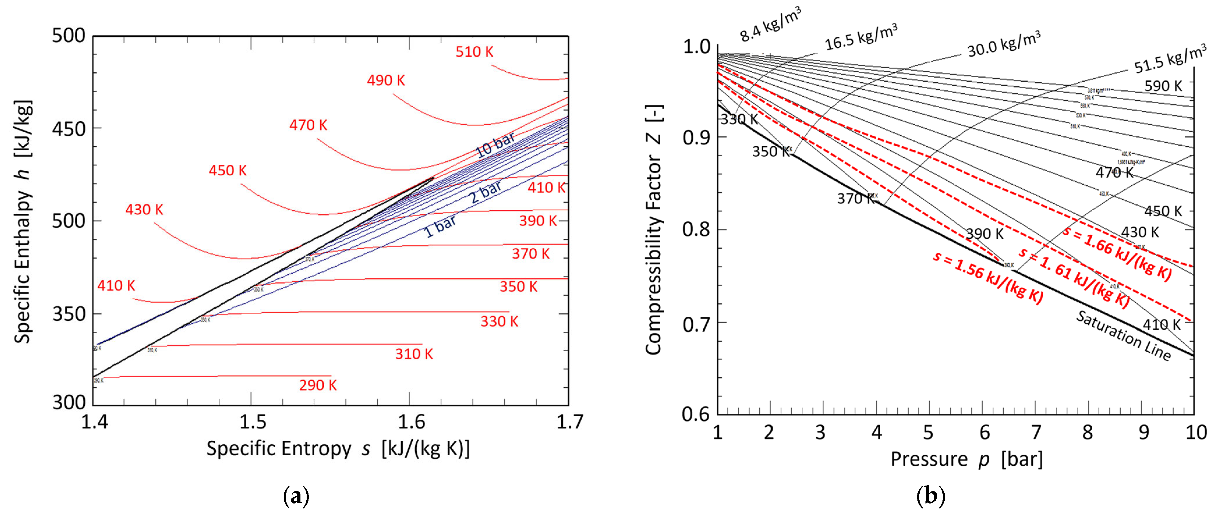
The non-toxic organic vapor NOVEC 649 (fluoroketone) by 3M was selected as a testing fluid. The molecular mass of Novec is 316 g/mol, and the critical point is at 18.8 bar and 442 K. The
h-s-diagram of NOVEC 649, in
Figure 2a, demonstrates that this organic vapor is a dry fluid defined by an overhanging two-phase region. Its thermodynamic behavior represents a broad working fluid class for ORC power systems. The
Z-p-diagram, in
Figure 2b, illustrates that NOVEC 649 is a non-perfect gas because its compressibility factor
Z is not a unique function of the specific entropy
s. If so, the (red) lines
s = constant must be horizontals in
Figure 2b, which is not the case. As discussed in detail by Traupel [
14] or by aus der Wiesche [
15], a fluid with
Z =
Z(
s) is formally equivalent to a perfect gas in terms of turbine cascade aerodynamics. If this condition is violated, which is obviously the case for NOVEC 649 for pressures between 1 bar and 10 bar, its aerodynamics cannot be formally described by perfect-gas dynamics. The operation points for the present case study were given by a constant stagnation temperature of
To = 370 K and prescribed density levels of
ρ = 30 kg/m
3 and 16.5 kg/m
3, respectively.
Table 1 compares the physical properties of air (at standard atmospheric conditions) and NOVEC 649. The thermodynamic properties of NOVEC 649 were evaluated using REFPROP at a pressure level of 2.5 bar and a temperature of about 97 °C representing typical ORC operation and testing conditions. The significant difference between the isentropic exponents (i.e., the ratio of the specific heats) between air and NOVEC 649 is striking.
The fundamental derivative of gas dynamics
Γ is suitable for classifying gas dynamics [
15]. A perfect gas exhibiting classical gas dynamics is characterized by
Γ = (
γ + 1)/2. This holds for dry air under atmospheric conditions. Classical but non-ideal gas dynamics correspond to 0 <
Γ < 1. This is achieved for NOVEC 649 under the thermodynamic conditions in
Table 1. The existence of fluids exhibiting non-classical gas dynamical phenomena with
Γ < 0 is still open [
15].
3. Experimental Setup
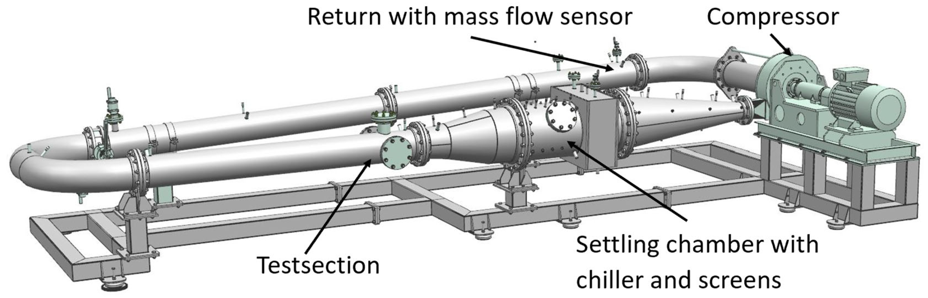
The present experimental investigation used the closed-loop organic vapor wind tunnel (CLOWT) at Muenster University of Applied Sciences, shown in
Figure 3. Details about this test facility and its capabilities for cascade experiments can be found in a recent study (Hake et al. [
13]) or in a review [
15] of test facilities and measurement techniques for non-ideal compressible fluid dynamics.
A centrifugal compressor drove the working fluid through the closed-loop wind tunnel. The settling chamber was equipped with a chiller to maintain stable total temperature conditions during operation (during the start-up stage, the entire wind tunnel was electrically heated to the desired temperature level). A multi-stage turbulence screen set and a two-stage contraction led to inflow turbulence levels of order 1%. The turbulent macro length
Λ (obtained using hot-wire anemometry, see following subsection) was of order 1 up to 2 mm in the test section. This corresponded to a normalized turbulent length scale
Λ/
c of order 3 × 10
−2 up to 6 × 10
−2, much larger than the normalized roughness of
ks/
c = (4.0 ± 0.5) × 10
−4. The linear turbine cascade was placed in the wind tunnel’s test section. The details of the cascade test section of the present investigations are shown in
Figure 4.
The present work represents a direct continuation of the previous study [
13] employing a modified cascade test section and new measurement techniques. The main differences from the previous study were: (i) the downstream domain of the cascade was significantly enlarged so that periodicity was ensured and the risk of a stagnation point flow at an end wall downstream of the cascade was prevented during the present measurements, (ii) profile pressure distributions were also obtained for the airfoils, (iii) hot-wire anemometry was employed in addition to the pressure measurements, and (iv) the movement of the probes and potential vibration issues in the streams of the high-density organic vapors were observed using optical access to the cascade test section and by employing a high-speed camera.
3.1. Instrumentation
The static pressure
p0 and the total temperature
To0 were measured at fixed positions in the wind tunnel’s settling chamber (denoted by subscript
0). During operation, the mass flow rate
was measured at the return of the closed-loop wind tunnel, as seen in
Figure 3. At the beginning of the high-speed test section (i.e., at the upstream station of the cascade denoted by subscript 1), the inflow static wall pressure
p1 was obtained via a static pressure tap placed centrally at the entrance to the cascade test section. Further static wall pressure taps were located at the end walls of the central blade passage of the cascade. Total pressures
po1(
y) and
po2(
y) were measured in the centerline of the cascade at upstream and downstream stations employing Pitot probes (tip diameter 1 mm, stem diameter 3 mm) along the traverse coordinate
y. The upstream station 1 was placed one axial chord upstream of the blade leading edge. The axial distance of downstream station 2 to the trailing edge of the blades was
x/
c = 0.07.
In addition to the Pitot probes, hot-wire measurements were conducted using a single wire (length 4 mm, diameter 10 µm, oriented parallel to the blade trailing edge) and a constant-temperature anemometer system. The calibration of hot-wire probes in the compressible flow of an organic vapor required substantial efforts, as Hake et al. [
16] discussed in more detail. In the present study, a fixed stagnation temperature
To0 = 370 K during the experiments avoided the need to determine the temperature sensitivity coefficient during calibration. The high wire Reynolds number (of order 1000) and the fixed wire over-heat ratio of 1.6 ensured that the density and velocity sensitivity coefficients were identical for the used hot-wire probe [
16]. That fact made the data reduction and interpretation of the electrical hot-wire signals easier, although compressibility effects were present.
3.2. Experimental Procedure
Before the experiments, the entire wind tunnel facility was evacuated and then filled with NOVEC 649 mass, yielding the desired density level (so-called inventory forward-control approach). The heating of the wind tunnel using an electrical heating system and the temperature control system working with an additional chiller in the settling chamber enabled a stable total temperature level To0 during the experiments. The temperature drift rate during a measurement campaign was only 10−3 K/s. The desired exit Mach number M2 was mainly controlled using the variable wind tunnel compressor running speed, which was continuously adjustable via the electrical frequency converter. The actual Reynolds number Re was primarily governed by the velocity (i.e., the Reynolds number was strongly linked to the Mach number) and slightly affected by the actual test section density.
Before the experiments with the organic vapor started, tests and instrumentation checks with air at atmospheric conditions were conducted. In the first set of experiments, the pressure measurements, including the traversing of the Pitot probes, were carried out. Based on these data, Mach number, flow velocity, and density were determined utilizing the static pressure, temperature, and mass flow rate data. Then, the Pitot probes were replaced with hot-wire probes, and the hot-wire measurements were carried out at the upstream and downstream stations for the same exit Mach numbers in the second set of experiments. At the central position of the blade passage, the velocity and density data obtained in the first set were used to calibrate the hot-wire probe using a semi-empirical King law (for details see Hake et al. [
16]). During the hot-wire measurements, the potential vibration of the probe was checked using a high-speed camera and optical access through a transparent end wall of the cascade. The visual inspection identified a significant probe vibration issue at high subsonic flow (
M2 > 0.6) caused by the high dynamic load on the probe stem. The optically determined vibration frequencies acted as outer disturbances while interpreting the hot-wire signals at higher Mach numbers.
3.3. Data Reduction and Uncertainty Analysis
The primary goal of the present study was the determination of the profile loss of the turbine cascade. Among the various methods for expressing the loss, the present study used the pressure loss coefficient
Y
and the energy loss coefficient
ζRegarding the reference pressure,
pref, in Equation (1), different definitions are available in the literature. Here, the definition
pref =
po2 −
p2 was used, as proposed by Horlock [
17]. The definition of the energy loss coefficient followed Kiock et al. [
11]. The averaging of the pressure loss coefficient was performed using the mass-flow averaging procedure for the total pressure difference, as Horlock [
17] described. The average reference pressure was obtained using the mass-flow averaged total exit pressure value and the area-averaged static exit pressure value. A similar procedure was applied for the averaged energy loss coefficient
ζ.
The energy loss coefficient
ζ and the pressure loss coefficient
Y were compared and converted using the simple ideal gas relation
with
γ as the isentropic exponent and
M2 as the exit Mach number. It might be noticed that Equation (3) is the first part of a power series for the Mach number of the exact conversion formula. Its deviation from the precise relationship between
ζ and
Y involving thermodynamic calculations for the real gas behavior was less than 2% for the present study at the highest Mach number.
All thermodynamic variables were obtained using the fluid database program REFPROP developed by NIST using the pressure and temperature measurements. For the Pitot probe data reduction, the scheme and the program explained in detail by Gori [
18] and Conti [
19] were applied. The relative uncertainty level of the pressure measurements was of order ∆
p/
p = 0.5% up to 1.6%. This level was mainly given by bias errors caused by the unknown hydrostatic pressure due to potential condensation in the pressure lines (see reference [
15] for a detailed discussion about the issues caused by condensation in pressure lines). The relative temperature uncertainty level was only ∆
T/
T = 0.06% up to 0.1%. The maximum local pressure coefficient uncertainty was ∆
Y = 0.0142 (in the wake). A maximum uncertainty of about ∆
Yav = 0.006 was achieved for the averaged loss coefficients due to the large number of sampling data for averaged quantities. The relative uncertainty levels for Reynolds and Mach numbers were 1%.
4. Considered Literature Loss Models
Among the many different loss models and correlations available in the open literature, the following frequently used and representative loss models were selected:
Soderberg’s correlation (see Horlock [
17] or Dixon and Hall [
20])
Although the considered loss models are somewhere out-dated, they are still in use in industry and academia. Furthermore, using a modern loss correlation would not provide an advantage for the present airfoil designed using methods of the late 1960s. The selection of the loss models covered the two empirical classical approaches used by Soderberg and Ainley and Mathieson (and its follow-up by Kacker and Okapuu) as well as the analytical boundary layer flow approach represented by the loss model proposed by Baljé and Binsley. The Traupel loss model might be considered a practical combination of empirical and analytical data. It is provided in parts in graphical form. For a deeper discussion of potential Reynolds number and roughness effects and for predicting the trailing edge loss contribution, Denton [
22], Aungier [
6], and Cheon et al. [
23] were consulted as sources, too.
Soderberg proposed a relatively simple method for estimating turbine cascade losses in the late 1940s [
17,
20]. His correlation was intended to predict the total loss for turbine cascades, but, considering the limit case for an infinite blade height
b/
H → 0, it could predict profile losses, including trailing edge losses [
17]. The Soderberg correlation is essentially a quadratic function of the deflection angle
ε =
β1 +
β2, and the Reynolds number correction follows the power law with
Re−1/4. In its original version, no roughness effects were included.
Ainley and Mathieson reported a method for estimating the performance of axial-flow turbines in the early 1950s [
1,
17,
20] based on individual loss contributions (profile loss, secondary loss, and tip clearance loss). Their approach has been widely used ever since, and several authors (e.g., [
4,
6,
8]) have modified their basic scheme but kept the main ideas. Ainley and Mathieson obtained their loss data for a nominal Reynolds number
Re2 = 2 × 10
5, and they recommended that the total-to-total efficiency
ηtt of the turbine stage should be corrected for lower Reynolds numbers according to
Compressibility and roughness effects were not included in the original version of the Ainley and Mathieson correlation. Kacker and Okapuu [
8] modified the Ainley and Mathieson loss system, among other things, by reducing the profile loss base level by a factor of three, introducing compressibility effects, and modifying the Reynolds number correction.
A profile loss correlation proposed by Baljé and Binsley [
21] was selected to represent a loss model based on the boundary-layer theory. Their profile loss coefficient ζ includes the trailing edge loss. The profile loss can be obtained using the boundary-layer theory expression
Here,
θ* denotes the normalized boundary layer momentum thickness quantity
θ* = (
θ/(
t sin
β2), and
δ* =
Hθ* can be computed using the shape factor
H of the boundary layer. For turbulent flow, a value of H = 1.4 was used. The Reynolds number correction is implemented via the correlation for the momentum thickness
θ. The latter depends on the blade angles and Re. In its original version, roughness effects were not explicitly covered but could be introduced by modifying the boundary layer quantities
δ* and
θ* utilizing suitable roughness correlations [
14,
24]. The pure boundary layer loss
ζBL can be estimated using a vanishing trailing edge thickness (
tTE = 0) in Equation (5).
5. Results and Discussion
The actual turbine cascade consisted of only three full airfoils, as seen in
Figure 4. Hence, it was necessary to check the periodicity for the central airfoil where the flow measurements and loss determinations were mainly performed. The exit domain and the guiding side contours were developed based on prior computational fluid dynamics solutions. The static pressure measurements downstream of the central airfoil indicated a high degree of periodicity:
p2(
y) was essentially identical to
p2(
y +
t) at different traverse positions
y (the deviations between the pressure measurements were within the experimental uncertainty level). The inflow uniformity was checked using a Pitot probe traversed at the upstream station. It was found that the total pressure
po1(
y) remained essentially constant, as reported in the previous study [
13].
Figure 5 shows an example of the measured total pressure and turbulence intensity distributions downstream of the central blade obtained for an exit Mach number of
M2 = 0.68. Similar results were obtained for other exit Mach numbers
M2 or Reynolds number levels. The wake downstream of the airfoil’s trailing edge is expressed by the local total pressure difference distribution ∆
po(
y) =
po1 −
po2 (black dots in
Figure 5) because the upstream total pressure
po1 is constant along the corresponding inflow traverse coordinate
y. The grey squares in
Figure 5 represent the measured normalized downstream turbulence intensities obtained using hot-wire anemometry (HWA). Here, the measured data are corrected concerning the finite wire length which is described in more detail in [
25,
26]. The agreement between the new HWA turbulence data for NOVEC 649 with the literature data [
27] obtained using laser-Doppler anemometry (LDA) for air was reasonable. This agreement supports the hypothesis that real gas effects are not dominating the turbulence at this Mach number level.
The averaged profile loss coefficient
ζ is plotted against the exit Reynolds and Mach numbers in
Figure 6. In addition to the new experimental data obtained for NOVEC 649, the literature data (see Kiock et al. [
11]) obtained for air at a fixed Reynolds number
Re2 = 0.8 × 10
6 but for various Mach numbers
M2 are shown in
Figure 6 for a better orientation. The literature loss data in
Figure 6 correspond to smooth airfoils, whereas the new NOVEC 649 data are measured for a rough blade (
ks/
c = 4 × 10
−4).
The prediction of the Traupel [
14] loss system is plotted as empty red symbols in
Figure 6, too. In the case of air and smooth blades (red symbols in
Figure 6), the agreement between the literature data and Traupel’s prediction is excellent. The Reynolds number effect (i.e., an increase in loss for decreasing Reynolds numbers) was predicted by Traupel for exit Reynolds numbers
Re2 < 0.5 × 10
6. Interestingly, the NOVEC 649 data point obtained for such a Reynolds number exhibited a significant increase in loss in comparison to the relatively stable loss level obtained for higher Reynolds numbers. The Reynolds number correction for the Soderberg correlation predicted a slight loss decrease with increasing Reynolds numbers. The profile loss level predicted by Soderberg was in remarkable agreement with the experimental data obtained for NOVEC 649 at higher Reynolds numbers. The original Baljé and Binsley method for smooth blades underestimated the profile loss for NOVEC 649 and rough airfoils. Still, a roughness correction of the boundary layer quantities (see
Section 4) led to a reasonable agreement in
Figure 5 (except for the low Reynolds number data point as in the case of Traupel).
In
Table 2, the predictions of all considered loss models are listed for the literature data point (air, smooth blades,
Re2 = 8 × 10
5).
Table 2 contains a loss breakdown in the boundary layer and trailing edge loss contributions.
Table 3 shows the same for NOVEC 649 obtained at
M2 = 0.68 and
Re2 = 3.2 × 10
6 for the rough airfoils.
The original loss models from Soderberg, Ainley and Mathieson [
1], Kacker and Okapuu [
8], and Baljé and Binsley [
21] considered only smooth blades. To cover roughness effects, these models were modified using the correction factor for roughness effects proposed by Cheon [
23]. The Traupel [
14] loss model already contained roughness effects. For the boundary layer calculation required by the Baljé and Binsley [
21] method, the same roughness model was used for calculating the momentum thickness. In the case of smooth blades and airflow at a relatively usual Reynolds number level, the Traupel [
14] and the Baljé and Binsley [
21] profile loss predictions were very close to the experimental value (see
Table 2). Significant deviations occurred in the case of a flow of NOVEC 649 through rough blades (see
Table 3 or
Figure 6). The agreement between the Soderberg [
20] correlation and the experimental data for NOVEC 649 at higher Reynolds or Mach numbers was remarkable, but in the case of lower Reynolds numbers, the Soderberg [
20] correlation failed. The Traupel [
14] and the Baljé and Binsley [
21] correlations predicted profile losses for NOVEC 649, which were in the same order as the observed losses. They were able to describe the observed increase at lower Reynolds numbers qualitatively, but they failed regarding the absolute values. It can be argued that flow separation occurs at the rough airfoils at lower Reynolds numbers (see also the observation reported in [
28]), and the boundary layer flow models do not adequately cover that phenomenon.
Table 2 and
Table 3 demonstrate that the trailing edge contribution to the profile loss is considerable. Substantial deviations regarding the trailing edge loss contribution exist for the literature loss correlations. That underlines the importance of more detailed investigations of trailing edge flows. It would be precious to separate the boundary layer profile loss contribution from the trailing edge flow contribution, but the present experimental setup did not permit such a breakdown. Some base pressure measurements and hot-wire anemometry (HWA) investigations were conducted in the present study.
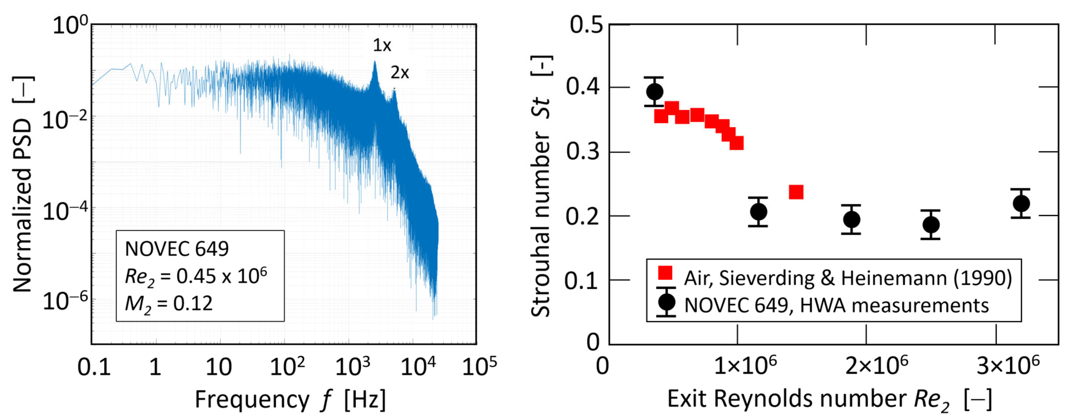
Figure 7 (left) shows a fast Fourier transform (FFT) generated power spectrum density (PSD) sample obtained for NOVEC 649. The recorded hot-wire signals served as a basis for the PSD. Since the focus was on the determination of the vortex shedding frequencies, no further correction schemes for the hot-wire signal were necessary to identify the characteristic vortex shedding frequencies
fTE. Clearly, the vortex shedding frequency
fTE (1x) and its double (2×) can be seen in the spectrum of the hot-wire signal in
Figure 7. Since the hot-wire anemometry was not sensitive against the flow direction, the double of the vortex shedding frequency occurred in the spectrum. Based on the fundamental trailing edge vortex shedding frequencies, the corresponding Strouhal number
was calculated and plotted against the exit Reynolds number in
Figure 7 (right). The literature data [
29] obtained for air and the same cascade (with a rounded trailing edge) are plotted in
Figure 7, too.
The present experimental data for NOVEC 649 agreed with the literature from Sieverding and Heinemann [
29]. It should be remarked that the present NOVEC 649 measurements covered an exit Mach number range of
M2 = 0.1 up to 0.7, whereas Sieverding and Heinemann [
29] considered
M2 = 0.3 up to 0.9. Due to the high density of NOVEC 649, the present Reynolds number range was larger but still comparable with the literature data. The new data supported the hypothesis that the Reynolds number was the dominant quantity for the vortex shedding frequency and not the Mach number. For higher Reynolds numbers, the Strouhal number was of order 0.2, as observed by Sieverding and Heinemann, whereas a substantially higher Strouhal number was noticed for lower Reynolds numbers. Future research is needed to extract the role of compressibility (i.e., the Mach number) on the trailing edge vortex shedding and its loss contribution.
The measured base pressure coefficient
Cp,bp = (
pTE −
p2)/(
po2 −
p2) at the trailing edge was about −0.05 + 0.01 at
M2 = 0.68 which was in agreement with the literature data obtained for air (Kiock et al. [
11]). This observation indicated that real gas effects were not of primary relevance to trailing edge vortex shedding for the actual subsonic flow. For lower exit Mach numbers,
M2 < 0.52, the base pressure coefficient was close to zero (with a tendency to increase slightly for
M2 tending to zero).
An interesting question is whether specific loss models are needed for real gas flows instead of the conventional loss systems obtained for ideal gas flows. At present, the few available data do not permit a final statement. Future research and an extension of cascade configurations are needed to close that gap. However, the present study [
30] represents a first step in this direction and can serve as a case study.
6. Conclusions
Based on the conducted experimental case study using rough blades and the organic vapor NOVEC 649 under subsonic flow conditions, the following conclusions can be drawn:
Whereas specific literature correlations (e.g., Traupel [
14]) can predict reasonable profile losses for smooth blades, accounting for roughness effects is still challenging. However, boundary layer theory models (e.g., Baljé and Binsley [
21]) have a high potential for predicting profile losses for non-separated flows. In any case, the careless use of classical loss models (e.g., Soderberg [
17,
20], Ainley and Mathieson [
1], Kacker and Okapuu [
8], Aungier [
6]) should be avoided for organic vapor flows in turbomachinery without further experimental proof or validation even for subsonic flow. Based on the present case study, using the simple robust Soderberg correlation for preliminary design is not worse than considering more sophisticated loss systems like Kacker and Okapuu [
8] or Aungier [
6].
Significant loss prediction deviations can occur with respect to the trailing edge contribution. For a relatively thick trailing edge, some of the loss models predicted relatively high contributions, which seemed to be questionable (e.g., Kacker and Okapuu [
8]). It was found that the exit Reynolds number governed the vortex shedding frequency, and dominant compressibility effects were not observed for
M2 < 0.68. This supports the hypothesis that boundary layer flow features characterized by the Reynolds number, not compressibility effects, are the dominating features for trailing edge vortex shedding under subsonic flow conditions. In the case of higher Mach numbers, transonic vortex shedding and compressibility effects and acoustic waves might substantially contribute to the profile loss.


