Comparative Study of Ant Colony Algorithms for Multi-Objective Optimization


1
School of Information Science and Engineering, Shenyang Ligong University, Shenyang 110159, China
2
School of Computer Science and Engineering, Northeastern University, Shenyang 110819, China
3
Department of Computer Science, IOWA State University, Ames, IA 50010, USA
4
Sam’s Club Technology Wal-mart Inc., Bentonville, AR 72712, USA
*
Author to whom correspondence should be addressed.
Information 2019, 10(1), 11; https://0-doi-org.brum.beds.ac.uk/10.3390/info10010011
Submission received: 29 October 2018
/
Revised: 12 December 2018
/
Accepted: 17 December 2018
/
Published: 30 December 2018
(This article belongs to the Section Artificial Intelligence)
Abstract
:In recent years, when solving MOPs, especially discrete path optimization problems, MOACOs concerning other meta-heuristic algorithms have been used and improved often, and they have become a hot research topic. This article will start from the basic process of ant colony algorithms for solving MOPs to illustrate the differences between each step. Secondly, we provide a relatively complete classification of algorithms from different aspects, in order to more clearly reflect the characteristics of different algorithms. After that, considering the classification result, we have carried out a comparison of some typical algorithms which are from different categories on different sizes TSP (traveling salesman problem) instances and analyzed the results from the perspective of solution quality and convergence rate. Finally, we give some guidance about the selection of these MOACOs to solve problem and some research works for the future.
1. Introduction
With the development of cloud computing and big data, the optimization problems we face becomes more and more complicated. In many cases, we need to consider several conflicting objectives and satisfy a variety of conditions. Such problems can be modeled well as multi-objective optimization problems (MOPs) [1,2,3]. This makes research on the solution to MOPs more important, and has become a hot topic in the field of intelligent optimization. In the last two years, evolutionary journals such as IEEE Transactions on Evolutionary Computation have published a large number of related research results. For MOPs, the Pareto Set (PS)/Pareto Front (PF) is the theoretical best solution. All the solutions in PF are non-dominated. Without the decision maker’s preference information, all the solutions are equally good [4]. A variety of algorithms has been designed to solve MOPs better. Most of them are non-complete algorithms, in which the meta-heuristic algorithms are focused on solving MOPs. These algorithms include multi-objective particle swarm optimization algorithms [5,6], multi-objective bee colony algorithms [7,8], multi-objective evolutionary algorithms [9,10], multi-objective genetic algorithms [11,12], multi-objective ant colony algorithms etc. [13,14]. When solving the discrete path multi-objective optimization problem, the multi-objective ant colony optimization algorithm (MOACO) is used more often than other heuristic algorithms, especially in solving variable-length path planning problems [15,16]. In this case, the ant colony optimization algorithm has unique advantages. Compared with the other related algorithms, it is more efficient. This is mainly because the construction graph used in the ACO algorithm can make the search space represented less redundant. Moreover, it has less parameters and strong robustness. When it is applied to solve another problem, only a little modification is needed.
As a meta-heuristic intelligent optimization method, ACO algorithms use a distributed positive feedback parallel computing mechanism. Therefore, it is easy to combine with other methods, and has strong robustness [17]. Initially, an ACO algorithm is used to solve single-objective optimization problems [18,19,20,21]. Due to the outstanding performance in solving these problems, it is also used to deal with other complex problems [22,23]. I.D.I.D Ariyasingha and others [24] analyzed seven multi-objective ant colony algorithms in 2012. They performed a detailed comparative analysis of these algorithms on several traveling salesman problem (TSP) test cases. In order to avoid falling into local optimum, while strengthening the local search ability of ants, Zhaoyuan Wang et al. [25] re-modified the solution construction method of the ant colony algorithm to make it can minimize network coding resources better. Chia-Feng Juang et al. [26], optimized the structure and parameters of fuzzy logic systems using MOACO. Meanwhile, they applied the optimized system to the mobile robot of the wall tracking control. The ant colony algorithm was applied to select a service with the optimal or approximately optimal output by Lijuan Wang and others [27]. In this way, the process of reaching agreement among service designers, service providers, and data providers becomes automatic. Manuel Chica et al. [28], proposed an interactive multi-rule optimization framework to balance the time and the space assembly line. The framework consists of a g-dominated scheme and a multi-target ant colony algorithm of an advanced cultural gene. It allows decision-makers to obtain optimal non-dominated solutions through the interaction of reference points. Xiao-Min Hu et al. [29] proposed an improved ant colony algorithm, which can accurately select the sensor in a reasonable way to complete the coverage task. Thereby, this saves more energy to maintain the sensor working for a long time and achieves the purpose of maximizing the working hours of the wireless sensor. Jing Xiao and others [30] applied the MOEA/D-ACO (multi-objective evolutionary algorithm using decomposition and ant colony) algorithm to software project scheduling issues, and compared MOEA/D-ACO with the NSGA-II algorithm in multiple test cases. However, the solution produced by MOEA/D-ACO on hard test instances does not have a better approximation to PF than the NSGA-II algorithm. The MOEA/D-ACO algorithm takes less time to solve most of the test instances. Shigeyoshi Tsutsui et al. [31] parallelized the ACO on multi-core processors in order to obtain the non-dominated solution sets faster. Moreover, they made an experimental comparison on several instances of secondary allocation problems with different sizes, and obtained a good result. Kamil Krynicki et al. [32], solved many types of resource query problem successfully. They solved these problems by adding many pheromone dynamic matrices to the ant colony algorithm and splicing pheromone stratification (Dynamic pheromone stratification). Héctor Monclús et al. [33], solved the management optimization problem of a sewage treatment plant by mixing two types of ant colony algorithms. Ibrahim Kucukkoc et al. [34] successfully implemented a mixed mode parallel pipelined system by using flexible agent-based ant colony optimization algorithm.
MOACOs mainly use artificial ants to select the vertices in the graph. Ants choose the next point by using pheromone information and heuristic information on the edge. Through these processes, ants construct a complete path. When MOACOs are used to solve MOPs, firstly, the search space of the problem is expressed in the form of a construction graph. Then the problem is transformed into a path optimization problem. Ants construct a tour by selecting the vertices in the construction graph. All the solutions that ants have just constructed are added to the non-dominated set by a dominance relationship [2]. After several iterations, the non-dominated set can be approximated to PF. People have proposed many MOACOs which have different characteristics and advantages. The analysis of these tasks can not only provide a reference for the research into MOACOs, but also guide the better application of MOACO to solve practical problems.
In Section 2, we give the basic process of solving MOP by ant colony algorithm, and analyze the differences among the existing MOACOs. The third part compares the existing MOACOs from many points of view, and gives the characteristics of each type of algorithm. It then selects the typical algorithm in each class for a relatively detailed description. In the subsequent section, the applicability of various algorithms is compared. We select typical MOACOs from different categories, and use various methods to compare the quality and the speed of convergence on different scale multi-objective TSP test problems. Finally, we summarize the existing problems of the multi-objective ant colony algorithm, and provide details of the expansion of this work.
2. The Basic Process of Solving the Multi-Objective Optimization Problem (MOP) by the Ant Colony Algorithm
This section first explains the general steps of the ant colony algorithm for MOPs. The multi-objective ant colony algorithm has many differences in using the strategy, such as: single-group/multi-group ants, single-pheromone/multi-pheromone matrix, single-heuristic/multi-heuristic matrix etc. These strategies can influence either the process of solving the problems or the quality of the solutions. The main steps of the ant colony algorithm to solve the multi-objective optimization problem are very similar.
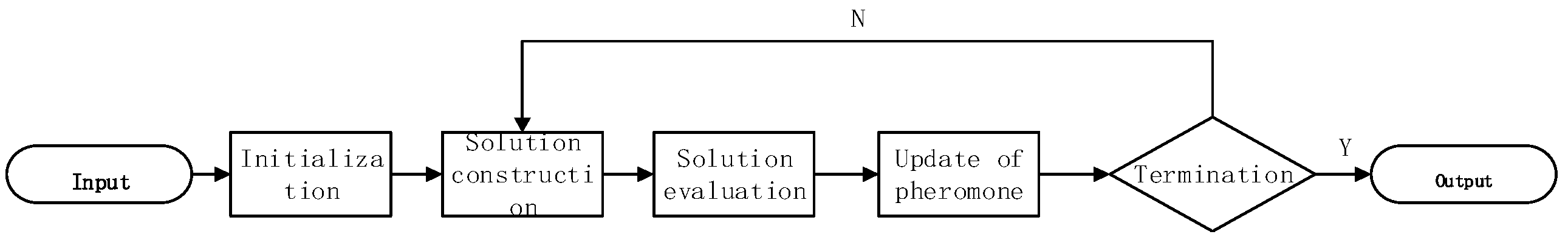
Through the study of the MOACOs algorithm in solving the multi-objective optimization problem, the basic process is shown in Figure 1.
The process the multi-objective colony algorithm takes in solving MOPs is generally divided into five steps:
- (1)
- Initialization: initialize the parameters of the algorithm, the pheromone information and heuristic information.
- (2)
- Solution construction: for each ant i, construct a new solution by using a probabilistic rule to choose solution components. The rule is a function of the current solution to sub-problem i, pheromone and heuristic information.
- (3)
- Solution evaluation: evaluate the solution of each ant obtained in step 2, store the non-dominated solutions, and eliminate the dominated ones.
- (4)
- Update of pheromone matrices: update the pheromone matrix by using information extracted from the newly constructed solutions. The pheromone related with edges in a non-dominated solution will increase.
- (5)
- Termination: if a problem-specific stopping condition is met, such as the number of iterations and the running time, the algorithm stops and outputs the non-dominated solution set, otherwise go back to step 2.
In the process of solving a multi-objective optimization problem, the difference of each ant algorithm is mainly reflected in step (1), step (2) and step (4). The differences in the initialization, solution construction, and the update of pheromone matrices, result in different improved MOACOs.
The differences in the initialization of ant colony optimization algorithms are mainly reflected in the following points: single-group/multiple-group, single-pheromone/multi-pheromone matrix, single-heuristic/multi-heuristic matrix and so on. Single-group/multi-group mainly refer to whether divide all the ants into single or multiple different groups. The single-group means that all the ants in one group share the same pheromone information and the same heuristic information in the algorithm. That is, the change of pheromone will affect all the solutions. Multi-group means that the ants in the algorithm are divided into many groups. Each group has its pheromone information matrix. The ants in the same group share one pheromone matrix and one heuristic matrix. The ants in the different group use different pheromone information. However, the groups are not unrelated, and they interact with each other through exchanging the solutions generated by the ant in its group, such as exchanging the non-dominated solutions generated by the marginal ants of the group. It is also possible to merge the non-dominated solutions generated by each group and then reassign them into each group. The main idea is to update the pheromone information of the group by using the non-dominated solution generated by other groups to achieve the purpose of cooperation. The single-pheromone/multi-pheromone matrix refers to the number of pheromone matrices that exist in the algorithm. The single pheromone matrix means that there is only one pheromone matrix in this kind of algorithms. All the ants share the same pheromone when they construct solutions, and also update the same pheromone matrix. The multi-pheromone matrices refer to the existence of more than one pheromone matrices in the algorithm. Each pheromone matrix corresponding to an objective, and each pheromone matrix will affect the construction of solutions. The algorithm aggregates multiple pheromones into a pheromone by means of weighted sum, weighted product, or random method. Whether all the ants share a pheromone matrix or ants in each group share a pheromone matrix directly affects the implementation of the algorithm subsequent steps. Similarly, the single-heuristic/multi-heuristic matrix refers to whether an algorithm uses one or more heuristic matrices. The single heuristic matrix refers to the fact that the algorithm has only one heuristic information matrix, and all the ants use the same heuristic information in the process of constructing the solution. The multi-heuristic matrix means that more than one heuristic information matrices exist in the algorithm. When constructing the solution, the algorithm must aggregate multiple heuristic information matrices into one heuristic information matrix, just like aggregating the pheromone information. The difference in the number of heuristic matrices also has a significant influence on the construction of the final non-dominated solution set. If using a single heuristic matrix, the non-dominated solution set is mainly an approximation to the central part of the Pareto Front. However, if using multi-heuristic matrices, the non-dominated solution set is an approximation to both ends of the Pareto Front [35].
There are many differences in the construction process of the ACO algorithm. Ants construct new solutions by using a probabilistic rule to choose which city to visit next. The rule is a function of pheromone information and heuristic information. This function is used to calculate the probability of visiting an unvisited city. Then the roulette wheel selection way is used to choose the city to visit next. The differences in the construction process of these algorithms are mainly reflected in the probability functions they use. They make ants choose paths differently, which directly influences the algorithm performance.
There are several strategies to choose when updating pheromone information. We can use different non-dominated solutions to update the pheromone matrix. For example, you can use all non-dominated solutions that have been generated so far to update the pheromone matrices. You can also use the non-dominated solutions generated in the current iteration to update the pheromone matrices. It is also possible to use the optimal solution generated in the current iteration of each weight vector to update the pheromone matrices. You can use the optimal solution related to each objective to update the pheromone matrices and so on. There are a variety of ways to update the pheromone. Just like the probability function, each different updating way directly affects the quality of the solution.
3. Classification of Multi-Objective Ant Colony Algorithms
In recent years, many excellent multi-objective ant algorithms have been proposed. We classify and analyze them from different aspects. The solving strategies they use are divided into two types: one is based on non-dominated ordering and the other is based on decomposition. The former determines the solution set according to the domination relations of each solution constructed by each ant. The probability function uses the weighted sum, weighted product, stochastic or other aggregation methods to construct. In this way, it can obtain more solutions. However, the solutions’ distribution is not uniform. They are usually concentrated in a specific direction. The latter decomposes a multi-objective optimization problem into a number of single-objective optimization problems, and gives a weight vector to each sub-problem. Each sub-problem stores a historical optimal solution in its direction. Then, sub-problems are solved simultaneously. This kind of method makes the distribution of the solutions more uniform, but the number of solutions may be lower.
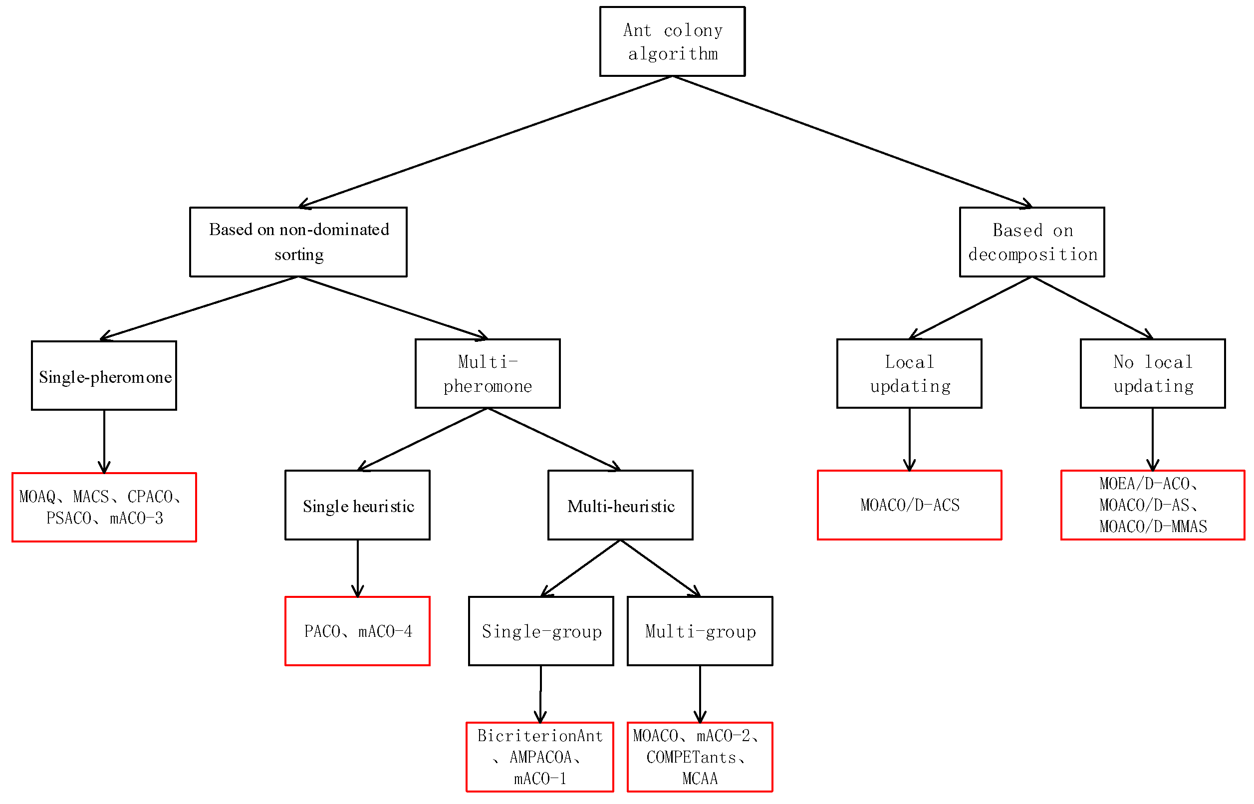
The specific classification of multi-objective ant colony algorithm is shown in Figure 2, in which the local update/no local update means whether pheromone is updated in the process of constructing solutions. For the local update way, every time an ant passes an edge, it will update the pheromone on it. The core idea is to reduce the probability of being selected by other ants, encourage other ants to explore a new edge, and finally increase the diversity of an ant’s selection. No local update means that the pheromone is not updated when ants construct solutions. After all the ants construct their solutions, the pheromone matrix is update. From it, we can intuitively understand the difference between the algorithms related to leaf nodes. Through different construction methods, there are different types of ant colony algorithm. The solution set achieved by these algorithms have great differences in solving the multi-objective TSP problem. As shown in this figure, the existing multi-objective ant colony algorithm is divided into two types. One is based on non-dominated sorting, and the other is based on decomposition. Different types of algorithm have great differences in the construction methods. The same class algorithms also have some differences. From all the leaf nodes, we select one or two algorithms to introduce its construction principle, and compare it with other types of algorithm.
3.1. Multi-Objective Ant Colony Algorithms Based on Non-Dominated Sorting
This kind of algorithm mainly adopts the strategy of non-dominated sorting in evaluating the solution. The solution of non-dominated solutions formed by this strategy may not be uniform, which corresponds to a part of PF. This kind of algorithm is divided into two types according to the number of pheromone matrices used.
3.1.1. Single-Pheromone Matrix
These algorithms mainly include MOAQ [36], MACS [37], CPACO [38], PSACO [39], mACO-3 [40] and so on. The MOAQ algorithm uses two heuristic matrices and two weights {0,1}. When the heuristic matrix corresponds to the weight vector {0,1} and {1,0}, we choose one from the two heuristic matrices. MACS can be seen as a variant version of MOAQ. The only difference between them is the number of weight vectors in aggregating heuristic information. MOAQ uses two weight vectors {0,1} and {1,0}, while MACS uses more than two weight vectors. The different number of weights has a great influence on the solution. The CPACO algorithm uses a state transition rule and a pheromone update rule different from MOAQ and MACS. And the incremental part is related to the level of each non-dominated solution. The PSACO algorithm is based on ant system (ant colony, AS [41]). The biggest change is about the pattern of pheromone updating rule. Two sets of solutions exist. One is the non-dominated solution set generated. The other is a fixed number of global optimal solutions. Through these two sets of solutions, the solution quality of each non-dominated solution set is calculated, and the result is applied to the pheromone update formula as a parameter. The mACO-3 uses one pheromone matrix, and its innovation is that pheromone on the same edge can only be updated once when iterating through a pheromone. We choose two representative algorithms from this type of algorithm.
MOAQ algorithm: the algorithm uses one pheromone matrix and two heuristic matrices. All ants share the same pheromone matrix. Each heuristic matrix is responsible for one objective. The MOAQ algorithm divides all the ants into two groups using two weights {0,1}. One uses the weight vector {1,0} and the other uses the weight vector {0,1}. This means that one group of ants uses only the first heuristic matrix, and the other one uses only the second heuristic matrix. This shows that the ants do not aggregate the two heuristic information matrixes of the two objectives, but rather that they choose one from the two. The algorithm uses all non-dominated solutions generated so far when updating the pheromone information.
MACS algorithm: this algorithm uses a pheromone matrix and many heuristic matrices. Each heuristic matrix is responsible for one objective. Each ant has a weight vector, and all heuristic matrices are aggregated by weighted product. The weight vectors between two ants are different, and all non-dominated solutions are used to update the pheromone information. MACS can be seen as a variant of MOAQ. The only difference between them is the number of weight vectors when aggregate heuristic information: MOAQ uses two weight vectors {0,1} and {1,0}, while MACS uses more than two weight vectors. This is because the different number of weights has a great influence on the algorithm. Therefore, this paper chooses these two algorithms for experimental comparison.
3.1.2. Multi-Pheromone Matrix
These algorithms are divided into two types based on the number of heuristic matrices used.
- (1)
- Single-heuristic matrix: the single heuristic matrix means that all ants in the algorithm share a heuristic matrix in the process of constructing the solution, including PACO [42], mACO-4 [40] and so on. The PACO algorithm is updated in a special way, using the best solution and second-best solutions to update pheromone information. The pheromone aggregation method used in mACO-4 is the same as mACO-1, but mACO-4 uses only one heuristic information matrix.
- PACO algorithm: this algorithm uses many pheromone matrices and one heuristic matrix. All ants share this heuristic matrix. Each pheromone matrix is responsible for one objective. As with the MACS, each ant has a weight vector, and all pheromone matrices are aggregated by using the weighted sum. This algorithm uses the best solution and second-best solutions of each objective to update pheromone information. The non-dominated solutions generated by the single-heuristic matrix mainly approximate to the central part of the Pareto Front [35].
- (2)
- Multi-heuristic matrix: this kind of algorithm uses a number of pheromone matrices and many heuristic matrices. According to the number of groups, these algorithms are divided into single-group and multi-group.
- (a)
- Single-group: the representative algorithms for this kind of algorithms are BicriterionAnt [43], AMPACOA [44], mACO-1 [40] and so on. Each ant in BicriterionAnt has a weight vector to aggregate pheromone information and heuristic information. AMPACOA is based on the first generation ant colony algorithm AS, and its characteristic is its pheromone updating way. This algorithm assigns a weight to each non-dominated solution based on the length of time when the non-dominated solution added. The weight is used to compute the coefficients of this non-dominated solution, and the coefficient of each non-dominated solution is related to the pheromone increment. The mACO-1 uses many ant groups. Each ant group is responsible for one objective, and it also has an additional ant group. It aggregates pheromone information and heuristic information of each ant group randomly by the weighted sum. The best solution for each group is used to update the respective pheromone matrices. The optimal solution for each objective generated by the additional group is to update the pheromone matrices of other groups.
- BicriterionAnt algorithms: this algorithm uses many pheromone matrices and many heuristic matrices, all of which are aggregated by the weighted sum. The number of weights equals the ants’, and each ant has a weight vector. When constructing the solution, the ants first calculate the probability of each untapped city by aggregating pheromone information and heuristic information. Then select the next city to go by roulette wheel selection. This algorithm uses the non-dominated solution generated by the current iteration to update the pheromone information.
- (b)
- Multi-group: this kind of algorithm differs from the single group in using more than one ant groups, including MOACO [45], mACO-2 [40], COMPETants [46], MACC [47] and so on. The MOACO algorithm uses multiple weights, but if the number of weights is less than the number of ants, the same weight may be used by different ants. The pheromone used by mACO-2 is the sum of the pheromones of all groups, rather than the weighted sum method used by mACO-1. The COMPETants algorithm divides the ants into three groups, each with a weight w = {0,0.5,1}. Each group of ants uses its weight vector to aggregate pheromone matrices and heuristic matrix to construct solution. The MACC algorithm divides the ants into multiple groups. Each group is responsible for one objective, and has its heuristic information and pheromone information. The pheromone matrice of each group is updated based on the best solution generated in the current iteration.
- MOACO algorithm: the MOACO algorithm uses multiple pheromone matrices and more heuristic matrices. Each pheromone matrix and heuristic matrix is responsible for one objective. All the ants are divided into many groups. Each group has multiple weights, and each ant in the group has a weight vector. If the number of weights in the group is less than the number of ants, the extra ants are assigned weights from the beginning. That is, it is possible that two or more ants in a group may use the same weight vector. The ant uses its weight vector to aggregate the pheromone information and heuristic information by the weighted product method. It then calculates the probability of the unvisited city to move to, and chooses the next city to visit by wheel roulette selection to construct the solution. Finally, it uses the non-dominated solution generated by current iteration to update the pheromone information.
3.2. Multi-Objective Ant Colony Algorithms Based on Decomposition
This kind of algorithm decomposes a multi-objective optimization problem into a number of single-objective optimization sub-problems. Each sub-problem has a weight. In this way, solving a multi-objective problem is transformed into solving multiple single-objective sub-problems, and each sub-problem has a best solution. The distribution of the non-dominated solution by this strategy is relatively uniform, but the number of non-dominated solutions is small. This algorithm has no local update in the process of constructing the solution. According to this, this kind of algorithm is divided into two types: local updating and no local updating.
3.2.1. Local Updating
This multi-objective ant colony algorithm is based on decomposition and ants use the local updating rule when they construct the solution. The representative of the algorithm is MOACO/D-ACS [48].
MOACO/D-ACS algorithm: this algorithm uses the Tchebycheff approach [49] to decompose a multi-objective problem into multiple single-objective sub-problems. Each sub-problem is assigned a weight vector, and this algorithm preserves the aggregated pheromone matrices and heuristic matrix before constructing the solution. Each ant may solve multiple sub-problems in an iteration, and more than one ants may solve a sub-problem. When constructing the solution, generate a uniformly random number from (0,1). If it is smaller than a control parameter, choose the city with the largest probability. Otherwise, select the city according to the roulette wheel selection. When updating the pheromone of the sub-problems, use the best solution of this sub-problem. Since in each iteration process, an ant may solve multiple sub-problems, it will result in multiple solutions. So there may be different pheromones that are updated by the same solution, and then the sharing of pheromone among sub-problems is better achieved. The MOACO/D-ACS algorithm adds a local updating rule. Ants visit edges and change their pheromone level by applying the local updating rule. The main idea is to reduce the probability of being selected by other ants, to encourage other ants to explore the new edges as well as increasing the diversity of ant selection.
3.2.2. No Local Updating
No local updating algorithms do not use the local updating rule when ants construct the solutions. They mainly include MOEA/D-ACO [50], MOACO/D-AS [48], MOACO/D-MMAS [48]. The MOEA/D-ACO algorithm allocates a number of neighbor ants for each ant based on the Euclidean distance of the sub-problem weights. This makes it easier for marginal neighbors in the different group to communicate, and increases the link within the group. The MOACO/D-AS algorithm is based on the decomposition and it combines the advantages of the MOACO/D [49] algorithm with the first-generation ant colony algorithm AS. MOACO/D-MMAS algorithm sets the maximum and minimum value of the pheromone and initializes the pheromone to the maximum value.
MOEA/D-ACO algorithm: after the ant colony algorithm based on decomposition, Liangjun Ke et al. combined the multi-objective evolutionary algorithm (EA) with an ant colony algorithm based on evolutionary decomposition. This algorithm decomposes a multi-objective optimization problem into a number of single-objective optimization problems by Tchebycheff approach. Each sub-problem has a weight vector, a heuristic information matrix, and an optimal solution. According to the Euclidean distance of the sub-problem weights, the ants are divided into groups and each ant has some neighbors. Each group has its pheromone matrix, and the ants in the same group share this pheromone matrix. Each ant is responsible for solving one sub-problem. Ants construct a new solution by aggregating the pheromone of its group, the heuristic information of the sub-problem and the optimal solution of the sub-problem. According to the objective function of the sub-problem, each ant uses the new solution constructed by its neighbors to update its optimal solution. This enables collaboration among different ant groups, since two neighbors may not be in the same group.
4. Experimental Comparisons of Typical Multi-Objective Ant Colony Algorithms
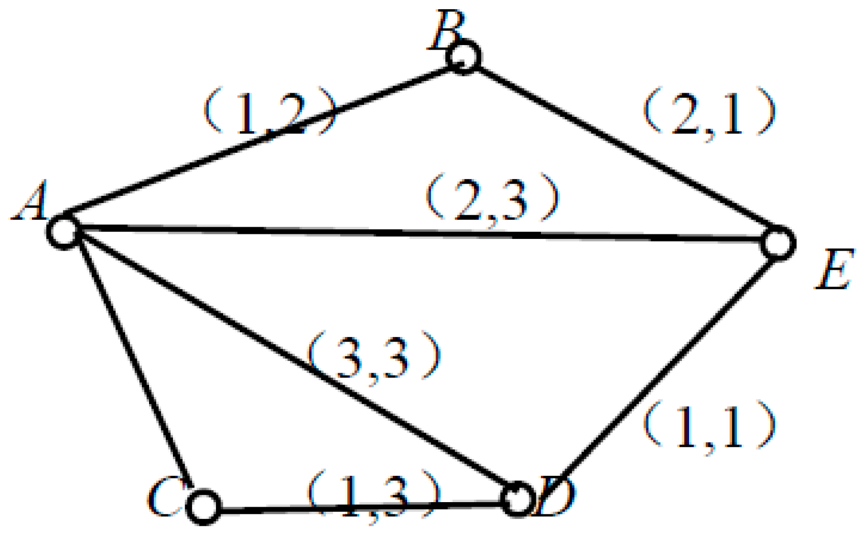
A very representative example of MOPs is the multi-objective TSP problem, which is often used as a benchmark for evaluating the performance of multi-objective optimization algorithms. This paper uses the standard multi-objective TSP problem as a study case and a test case to analyze the performance of MOACOs. It is defined as follows: a traveling businessman starts from one city. Each city must be visited and can be visited only once. After visiting all the cities, he needs to go back to the starting city. This problem is to find the shortest path. In this paper, the multi-objective TSP problem is taken as an example, and its structure chart is an undirected graph. In order to understand the multi-objective TSP problem better, Figure 3 gives an example. The (1,2) on the edge A→B represents the two different objective values (for example, the distance and time) of the multi-objective TSP problem. The distance and time on the edge B→A are the same as those on the edge A→B. Suppose a traveling businessman starts from city A and walks through all the cities in the graph, and each city must be visited and can only be visited once, then finally returns to city A. We want to find all the non-dominated solutions from the possible paths.
According to Figure 3, this is a specific multi-objective TSP problem example. The process of solving this problem by ant colony algorithm is as follows:
- Initialization: initialize the parameters of the algorithm, the pheromone information and heuristic information. Initialize the objective1, the objective2 and the pheromone τ on each edge. Such as edge (A, B) and initialize the parameters: α, β, λ, ρ etc. According to the weight λi, calculate the pheromone matrix τi and heuristic matrix ηi of each ant.
- Solution construction: each ant constructs a solution based on a probability function P consisting of pheromone information and heuristic information. Through the following probability function, each ant i constructs a path according to its τi and ηi.where C represents a set of all the cities that are connected with the city m and unvisited by the ant i.
- Solution evaluation: evaluate the solution of each ant in step 2. Store the non-dominated solution in the non-dominated solution set according to the relationship of dominance. Moreover eliminate the dominated solution.
- Update of pheromone matrices: updating pheromone information τ on all edges: If the edge is in the non-dominated solution, it is updated by pheromone increment. Otherwise, volatile the pheromone, that is, the pheromone increment is 0. The formula is as follows:where ρ is the volatilization factor and Δτ is the pheromone increment.
- Termination: determine the number of iterations whether met the max value or whether the runtime is over. If there is no end, return to step 2 to continue. Otherwise, output the set of non-dominated solutions, then the algorithm is ended.
In this paper, the comparison of these algorithms is done by solving the specific multi-objective TSP problem. In the experiment, we selected the seven algorithms described above: MACS, PACO, MOACO, MOACO/D-ACS, MOEA/D-ACO, and nine standard multi-objective TSP test cases [51] kroAB100, kroAC100, kroAD100, kroCD100, kroCE100, euclidAB100, euclidCE100, kroAB150, kroAB200 that can be downloaded from http://eden.dei.uc.pt~paquete/tsp/. The parameters of these algorithms are using the parameter settings in their respective algorithm papers. The MOEAD/ACO parameters are set as α = 1, β = 10, ρ = 0.95, τ = 0.9 and T = 10, where T is the swarm size. The MACS parameters are set as α = 0.9, β = 1.0, ρ = 0.1, T = 10. The PACO parameters are set as α = 1.0, β = 1.0, ρ = 0.1, τ = 1.0, T = 10. The MOACO parameters are set as α = 1.59, β = 2.44, ρ = 0.54, τ = 0.69, T = 10. The MOACO/D parameters are set as α = 1.0, β = 2.0, ρ = 0.02, Γ = 2, N = 20, where Γ is the number of ants in each sub-colony and N is the number N of sub-problems.
The performance of the algorithm has a great relationship with the number of ants and the size of the city. In order to avoid the algorithm from getting into the local optimum prematurely, it is important to let ants explore new paths. The formula for the termination of the algorithm which is generally used in the paper [50] is as following: N × 300 × (n/100)/2. Where N represents the number of ants, and n represents the number of cities. All the experiments are conducted in the same environment and implemented in the C language, and the MOEA/D-ACO algorithm was written by us. The original author provides the remaining six algorithm programs. We run 30 times for each algorithm to solve the same problem and compared the non-dominated solution set with the other algorithms by the hyper-volume indicator (H-indicator) [52,53,54] and the hypothesis test [54]. At the same time, the convergence of these algorithms including MOEA/D-ACO, MACS, MOACO/D-ACS, MOACO and PACO was analyzed on the test cases including kroAB100, kroAB150 and kroAB200 of different sizes. The performance of these algorithms is assessed based on the hyper-volume indicator in this paper, since it possesses the highly desirable feature of strict Pareto compliance. Whenever one approximation completely dominates another approximation, the hyper-volume of the former will be greater than the hyper-volume of the latter.
4.1. Comparison Based on H-Indicator
In this section, each algorithm runs 30 times independently based on the best parameter set in their paper under the nine test cases. Then we transform the experimental results of each algorithm into a H-indicator value. After that, the performance of each algorithm is analyzed by box plot and mean-variance table.
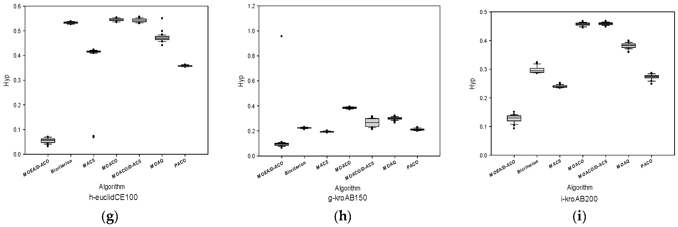
The box plots based on the H-indicator is shown in Figure 4. The H-indicators were obtained by seven algorithms solving the nine standard multi-objective TSPs. There are five solid lines and a dotted line in the box plot. The solid line from top to bottom successively represents the maximum point (there may be abnormal points), 1/4 digits, median, 3/4 digits, and minimum (there may be abnormal points). The dotted line represents the mean value. Because we want to find the minimum optimal value, the smaller the value of the H-indicator, the better the quality of the solution.
So through the box plots we can intuitively see which algorithm is better at solving the problem. If an algorithm has a smaller box value or a smaller mean value on the problem, we can determine the algorithm has better solutions on this problem. If these boxes are aggregated, it can be considered that the solution of the algorithm on this problem is relatively stable. Through the box plots of the nine questions above, it can be seen that the performance of the MOEA/D-ACO algorithm in solving these nine problems is better than the other six algorithms. However, in addition to the kroAD100, the MOEA/D-ACO algorithm is not as stable as most of the other algorithms on the other test cases.
The hyper-volume indicator is strictly monotonic and is widely used in the comparison of multi-objective optimization algorithms. This indicator determines the distance between the set of solutions with the Pareto Front by calculating the size of the volume between each solution set and the Pareto Front. If the solution is closer to the Pareto Front, the solution set is better, otherwise it is worse. We run each algorithm 30 times on each problem. We then transform the non-dominated solution set into H-indicator. Finally, we compare and analyze according to these four aspects: maximum (the smaller, the better), minimum, mean, standard deviation, as shown in Table 1 below.
It can also be seen from Table 1 that the MOEA/D-ACO algorithm has the minimum mean H value on each problem. The minimum value is best. In other words, the MOEA/D-ACO algorithm is the best. As for the maximum value, this is the best in most of the test cases except the kroAD100, kroCE100 and euclidAB100. However, regarding standard deviation, the performance of this algorithm is not good in most cases. This shows that the stability of this algorithm for these problems is weak, which is consistent with the conclusions of the box plots. Besides, we analyze the performance of each algorithm from six aspects. The six aspects are the maximum, the minimum, the mean, the standard deviation, the median and the quality of the solution (H-indicators as small as possible). At the same time, in every aspect of each problem, we have listed the best algorithm. The specific results are shown in Table 2.
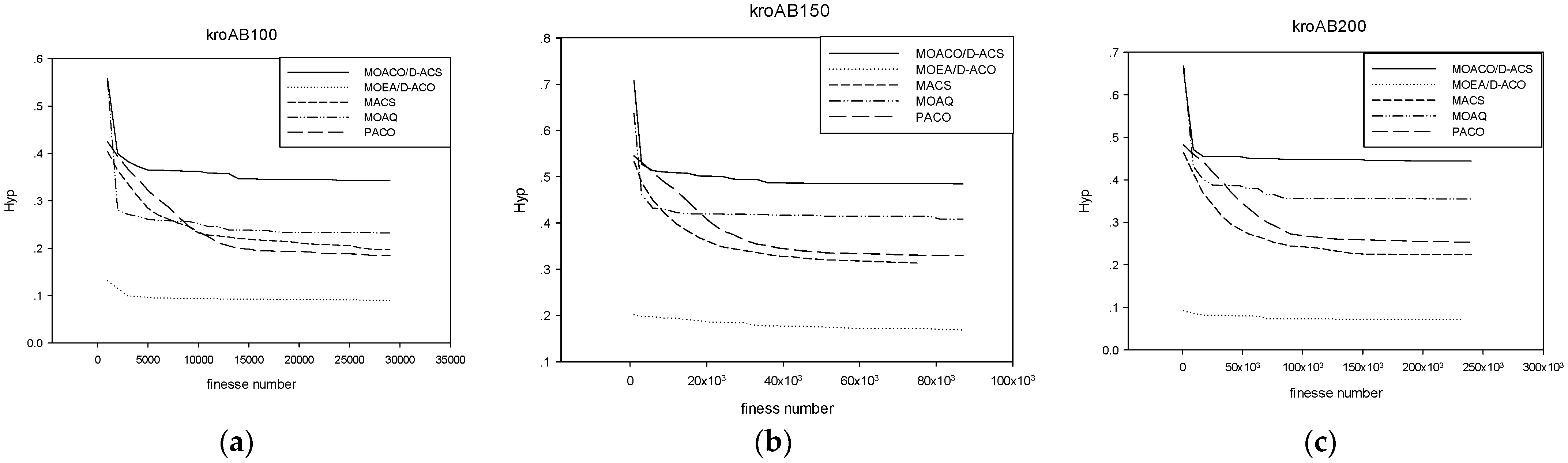
4.2. Convergence Analysis Based on H-indicator
In this part, several algorithms are selected for comparison. Moreover, the convergence analysis of these algorithms is tested in different scale test cases. The purpose is to obtain the number of maximum fitness evaluations of the algorithm in different scale test cases. Finally, we evaluated the performance of the algorithm after convergence. kroAB100, kroAB150, kroAB200 and other different scale cases are selected as test cases, MOACO/D-ACS, MOEA/D-ACO, MACS, MOAQ, PACO and so on are chosen as test algorithms.
As shown in Figure 5, the x-axis represents the number of fitness evaluations. With the size of the problem increasing, the number of fitness evaluations is also increasing. The y-axis represents the H-indicator value. As can be seen from the figure, with the increase in the scale of test cases, the location of convergence of each algorithm is also increasing.
4.3. Comparison of Hypothesis Testing
In order to determine the performance of each algorithm on the same problem more accurately, we use the statistical hypothesis test to analyze the H-indicator of each algorithm. The results are shown in Table 3, Table 4, Table 5, Table 6, Table 7, Table 8, Table 9, Table 10 and Table 11 below.
As shown in Table 3, Table 4, Table 5, Table 6, Table 7, Table 8, Table 9, Table 10 and Table 11 above, there are p values of the hypothesis test for each pair of optimization algorithms QR (row) and QC (column) on the same problem. When the p value of an algorithm A is smaller than the p-value of algorithm B by 0.05, it means that there is a significant difference. In other words, the solution of algorithm A is better than that of algorithm B. That is to say, algorithm A is better than algorithm B in solving this problem. From Table 3, Table 4, Table 5, Table 6, Table 7, Table 8, Table 9, Table 10 and Table 11, we find that for all test cases, the p-value of MOEA/D-ACO algorithm is smaller than that of the other algorithms by 0.05. It can be seen that the solution of the MOEA/D-ACO algorithm is better than the other algorithms in solving the same test case. This is consistent with the conclusion that we obtained by analyzing the box plots.
4.4. Approximate Pareto Front
In this part, we select three representative examples kroAB100, kroAB150, and kroAB200. By running these following algorithms 30 times independently, we obtain the approximate Pareto Fronts for the MOEA/D-ACO, MACS, MOACO, MOACO/D-ACS and PACO. From Figure 6, we can see that the solution set of MOEA/D-ACO algorithm on the first two test cases is better than other algorithms. Its solution set is more approximated to the PF. However, MOEA/D-ACO only approximates to a part of the Pareto Front, and the solution set of other algorithms is more comprehensive. In the third graph, the solutions of the two algorithms based on decomposition, MOEA/D-ACO and MOACO/D-ACS, are significantly better than those of other algorithms. However, the solution set of MOACO/D-ACS only approximate to the middle part of the Pareto Front.
It can be seen that the solution obtained by the MOACO algorithm based on non-dominated sorting can obtain more solutions and may approximate to a specific part of the Pareto Front. The distribution of these solutions is not uniform. By contrast, the solutions obtained by the MOACO based on decomposition can approximate to the Pareto Front more uniformly. This kind of algorithm only saves the best solution in each sub-direction. So, the number of solutions is lower. It can be seen from the recent related works that the research and application about MOACO based on decomposition has attracted lots of attentions and has become a hot topic in the multi-objective optimization area. However, in a specific situation, it is essential to consider which kind of multi-objective ant colony algorithm to choose in order to solve a problem and we should analyze the characteristics of the search space related with it. If the distribution of the Pareto Front is decentralized, the advantage of using an approach based on decomposition is more obvious.
5. Conclusions
Nowadays, theory and applied research on multi-objective ant colony optimization are continuously developing. Researchers have tried to use the algorithm for various practical engineering optimization problems. It has been shown that the multi-objective ant colony optimization algorithm has a definite advantage for the discrete space optimization problem. Besides, some researchers have tried to apply it to solve the multi-objective continuous optimization problem, and have also made achievements. In this paper, we provide the basic solving process of the multi-objective ant algorithm. Meanwhile, we analyzed the various multi-objective ant algorithms proposed in recent years from different aspects of solving strategies. We classified these algorithms completely and compared these algorithms regarding solving quality, solving efficiency, and so on. Although the multi-objective ant algorithm works well in solving the discrete combinatorial optimization problem, there are still many problems to be solved today, such as how to prevent ants from getting into the local optimal, the better approach to avoid the algorithm converging prematurely, the parameter setting of the algorithm. It is possible to collect a variety of data related to the optimization process itself during the operation of the algorithm. Therefore, effective information extracted from these data can guide the optimization process effectively. Thus using the operational information to guide the process of multi-objective ant colony optimization will be an effective way to improve its performance further. The number of optimization objectives is increasing because the optimization problem becomes more complicated. The phenomenon has made the study of the many-objective optimization problem more popular in the recent two years. Related research results into the many-objective optimization problem are also increasing rapidly. Therefore, how to use the ant colony optimization algorithm to solve many-objective optimization problems effectively is a future research direction. Moreover, related research on theoretical analysis is mainly for single objective ACO algorithms. Little research has been done for multi-objective ACO algorithms. So, research into the convergence analysis or explanation that can be proved for the multi-objective ACO algorithm or many-objective ACO algorithm is really needed.
Author Contributions
Software and validation, J.N.; conceptualization and supervision, C.Z.; data curation and writing—original draft preparation, P.S.; writing—review and editing, Y.F.
Funding
This research was funded by the Doctoral Startup Foundation of Liaoning Province (Grant No. 20170520197), and the national Natural Science Foundation Program of China (Grant No. 61572116 and 61572117).
Acknowledgments
Thanks for the support given by the China Scholarship Council (201806085015).
Conflicts of Interest
The authors declare no conflict of interest and the funders had no role in the design of the study.
References
- Wei, W.; Ouyang, D.T.; Lv, S.; Feng, Y.X. Multiobjective Path Planning under Dynamic Uncertain Environment. Chin. J. Comput. 2011, 34, 836–846, (In Chinese with English Abstract). [Google Scholar] [CrossRef]
- Kalyanmoy, D.; Himanshu, J. An Evolutionary Many-Objective Optimization Algorithm Using Reference-Point-Based Non-dominated Sorting Approach, Part I: Solving Problems with Box Constraints. IEEE Trans. Evol. Comput. 2014, 18, 577–601. [Google Scholar]
- Wen, R.Q.; Zhong, S.B.; Yuan, H.Y.; Huang, Q.Y. Emergency Resource Multi-Objective Optimization Scheduling Model and Multi-Colony Ant Optimization Algorithm. J. Comput. Res. Dev. 2013, 50, 1464–1472, (In Chinese with English Abstract). [Google Scholar]
- He, Z.N.; Yen, G.G. Visualization and Performance Metric in Many-Objective Optimization. IEEE Trans. Evol. Comput. 2016, 20, 386–402. [Google Scholar] [CrossRef]
- Ganguly, S. Multi-objective planning for reactive power compensation of radial distribution networks with unified power quality conditioner allocation using particle swarm optimization. IEEE Trans. Power Syst. 2014, 29, 1801–1810. [Google Scholar] [CrossRef]
- Yu, X.; Chen, W.N.; Hu, X.M.; Zhang, J. A Set-based Comprehensive Learning Particle Swarm Optimization with Decomposition for Multi-objective Traveling Salesman Problem. In Proceedings of the 2015 Annual Conference on Genetic and Evolutionary Computation, Madrid, Spain, 11–15 July 2015; pp. 89–96. [Google Scholar]
- Horng, S.C. Combining artificial bee colony with ordinal optimization for stochastic economic lot scheduling problem. IEEE Trans. Syst. Man Cybern. Syst. 2015, 45, 373–384. [Google Scholar] [CrossRef]
- Gao, W.F.; Huang, L.L.; Liu, S.Y.; Dai, C. Artificial bee colony algorithm based on information learning. IEEE Trans. Cybern. 2015, 45, 2827–2839. [Google Scholar] [CrossRef]
- Jara, E.C. Multi-Objective Optimization by Using Evolutionary Algorithms: The p-Optimality Criteria. IEEE Trans. Evol. Comput. 2014, 18, 167–179. [Google Scholar] [CrossRef]
- Cai, X.Y.; Li, Y.X.; Fan, Z.; Zhang, Q.F. An external archive guided multi-objective evolutionary algorithm based on decomposition for combinatorial optimization. IEEE Trans. Evol. Comput. 2015, 19, 508–523. [Google Scholar]
- Eldurssi, A.M.; O’Connell, R.M. A fast non-dominated sorting guided genetic algorithm for multi-objective power distribution system reconfiguration problem. IEEE Trans. Power Syst. 2015, 30, 593–601. [Google Scholar] [CrossRef]
- Cheng, Y.F.; Shao, W.; Zhang, S.J. An Improved Multi-Objective Genetic Algorithm for Large Planar Array Thinning. IEEE Trans. Magnet. 2016, 52, 1–4. [Google Scholar] [CrossRef]
- Zuo, L.Y.; Shu, L.; Dong, S.B.; Zhu, C.S.; Hara, T. A Multi-Objective Optimization Scheduling Method Based on the Ant Colony Algorithm in Cloud Computing. IEEE Access 2015, 3, 2687–2699. [Google Scholar] [CrossRef]
- Gao, L.R.; Gao, J.W.; Li, J.; Plaza, A.; Zhuang, L.; Sun, X.; Zhang, B. Multiple algorithm integration based on ant colony optimization for endmember extraction from hyperspectral imagery. IEEE J. Sel. Top. Appl. Earth Observ. Remote Sens. 2015, 8, 2569–2582. [Google Scholar] [CrossRef]
- Liu, Y.X.; Gao, C.; Zhang, Z.L.; Lu, Y.; Chen, S.; Liang, M.; Tao, L. Solving NP-hard problems with Physarum-based ant colony system. IEEE/ACM Trans. Comput. Biol. Bioinform. 2017, 14, 108–120. [Google Scholar] [CrossRef]
- Yu, Y.; Li, Y.; Li, J. Nonparametric modeling of magnetorheological elastomer base isolator based on artificial neural network optimized by ant colony algorithm. J. Intell. Mater. Syst. Struct. 2015, 26, 1789–1798. [Google Scholar] [CrossRef]
- Liu, Q.; Chen, H.; Zhang, Y.G.; Li, J.; Zhang, S.B. An Ant Colony Optimization Algorithm Based on Dynamic Evaporation Rate and Amended Heruistic. J. Comput. Res. Dev. 2012, 49, 620–627. [Google Scholar]
- Zeng, M.F.; Chen, S.Y.; Zhang, W.Q.; Nie, C.H. Generating covering arrays using ant colony optimization: Exploration and mining. Ruan Jian Xue Bao/J. Softw. 2016, 27, 855–878. Available online: http://www.jos.org.cn/1000-9825/4974.htm (accessed on 3 October 2017). (In Chinese with English Abstract).
- Lin, Z.Y.; Zou, Q.; Lai, Y.X.; Lin, C. Dynamic result optimization for keyword search over relational databases. Jian Xue Bao/J. Softw. 2014, 25, 528–546. Available online: http://www.jos.org.cn/1000-9825/4384.htm (accessed on 9 August 2017).
- Wen, Y.P.; Liu, J.X.; Chen, Z.G. Instance aspect handling-oriented scheduling optimization in workflows. Jian Xue Bao/J. Softw. 2015, 26, 574–583. Available online: http://www.jos.org.cn/1000-9825/4767.htm (accessed on 22 September 2017). (In Chinese with English Abstract).
- Wang, G.C.; Feng, P.; Wang, Z.; Peng, Y.; Huang, S.Q. Study on Engery Consumption Optimization Routing Strategy Based on Rate Adaptation. Chin. J. Comput. 2015, 38, 555–566. [Google Scholar]
- Wang, X.Y.; Choi, T.M.; Liu, H.K.; Yue, X.H. Novel Ant Colony Optimization Methods for Simplifying Solution Construction in Vehicle Routing Problems. IEEE Trans. Intell. Transp. Syst. 2016, 17, 3132–3141. [Google Scholar] [CrossRef]
- Hajar, B.T.; Ali, M.H.; Rizwan, M. Simultaneous Reconfiguration, Optimal Placement of DSTATCOM and Photovoltaic Array in a Distribution System Based on Fuzzy-ACO Approach. IEEE Trans. Sustain. Energy 2015, 6, 210–218. [Google Scholar]
- Ariyasingha, I.D.I.D.; Fernando, T.G.I. Performance analysis of the multi-objective ant colony optimization algorithms for the traveling salesman problem. Swarm Evol. Comput. 2015, 23, 11–26. [Google Scholar] [CrossRef]
- Wang, Z.Y.; Xing, H.L.; Li, T.R.; Yang, Y.; Qu, R.; Pan, Y. A Modified Ant Colony Optimization Algorithm for Network Coding Resource Minimization. IEEE Trans. Evol. Comput. 2016, 20, 325–342. [Google Scholar] [CrossRef]
- Juang, C.-F.; Jeng, T.-L.; Chang, Y.-C. An Interpretable Fuzzy System Learned Through Online Rule Generation and Multiobjective ACO with a Mobile Robot Control Application. IEEE Trans. Cybern. 2016, 46, 2706–2718. [Google Scholar] [CrossRef] [PubMed]
- Wang, L.J.; Shen, J. Multi-Phase Ant Colony System for Multi-Party Data-Intensive Service Provision. IEEE Trans. Serv. Comput. 2016, 9, 264–276. [Google Scholar] [CrossRef]
- Chica, M.; Cordón, Ó.; Damas, S.; Bautista, J. Interactive preferences in multiobjective ant colony optimisation for assembly line balancing. Soft Comput. 2015, 19, 2891–2903. [Google Scholar] [CrossRef]
- Liu, Y.; Chen, W.N.; Hu, X.; Zhang, J. An Ant Colony Optimizing Algorithm Based on Scheduling Preference for Maximizing Working Time of WSN. In Proceedings of the Genetic and Evolutionary Computation, Madrid, Spain, 11–15 July 2015; pp. 41–48. [Google Scholar]
- Xiao, J.; Gao, M.L.; Huang, M.M. Empirical Study of Multi-objective Ant Colony Optimization to Software Project Scheduling Problems. In Proceedings of the 2015 Annual Conference on Genetic and Evolutionary Computation, Madrid, Spain, 11–15 July 2015; pp. 759–766. [Google Scholar]
- Tsutsui, S.; Fujimoto, N. A Comparative Study of Synchronization of Parallel ACO on Multi-core Processor. In Proceedings of the 2015 Annual Conference on Genetic and Evolutionary Computation, Madrid, Spain, 11–15 July 2015; pp. 777–778. [Google Scholar]
- Krynicki, K.; Houle, M.E.; Jaen, J. An efficient ant colony optimization strategy for the resolution of multi-class queries. Knowl.-Based Syst. 2016, 105, 96–106. [Google Scholar] [CrossRef]
- Verdaguer, M.; Clara, N.; Monclús, H.; Poch, M. A step forward in the management of multiple wastewater streams by using an ant colony optimization-based method with bounded pheromone. Process Saf. Environ. Protect. 2016, 102, 799–809. [Google Scholar] [CrossRef]
- Kucukkoc, I.; Zhang, D.Z. Mixed-model parallel two-sided assembly line balancing problem: A flexible agent-based ant colony optimization approach. Comput. Ind. Eng. 2016, 97, 58–72. [Google Scholar] [CrossRef] [Green Version]
- López-Ibáñez, M.; Stützle, T. The impact of design choices of multiobjective antcolony optimization algorithms on performance: An experimental study on the biobjective TSP. In Proceedings of the 2015 Annual Conference on Genetic and Evolutionary Computation, Portland, OR, USA, 7–11 July 2010; pp. 71–78. [Google Scholar]
- García-Martínez, C.; Cordón, O.; Herrera, F. A taxonomy and an empirical analysis of multiple objective ant colony optimization algorithms for the bi-criteria TSP. Eur. J. Oper. Res. 2007, 180, 116–148. [Google Scholar] [CrossRef] [Green Version]
- Barán, B.; Schaerer, M. A Multiobjective Ant Colony System for Vehicle Routing Problem with Time Windows. In Proceedings of the 21st IASTED international Multi-Conference on Applid Informatics, Innsbruck, Austria, 10–13 February 2003; pp. 97–102. [Google Scholar]
- Angus, D. Crowding Population-based Ant Colony Optimisation for the Multi-objective Travelling Salesman Problem. In Proceedings of the 2007 IEEE Symposium on Computational Intelligence in Multi-Criteria Decision-Making, Honolulu, HI, USA, 1–5 April 2007; pp. 333–340. [Google Scholar]
- Thantulage, G.I.F. Ant Colony Optimization Based Simulation of 3D Automatic Hose/Pipe Routing; Brunel University: London, UK, 2009. [Google Scholar]
- Solnon, C. Ant colony optimization for multi-objective optimization problems. In Proceedings of the 19th IEEE International Conference on Tools with Artificial Intelligence (ICTAI 2007), Patras, Greece, 29–31 October 2007; Volume 1, pp. 450–457. [Google Scholar]
- Dorigo, M.; Maniezzo, V.; Colorni, A. Ant system: Optimization by a colony of cooperating agents. IEEE Trans. Syst. Man Cybern. Part B Cybern. 1996, 26, 29–41. [Google Scholar] [CrossRef] [PubMed]
- Doerner, K.; Gutjahr, W.J.; Hartl, R.F.; Strauss, C.; Stummer, C. Pareto ant colony optimization: A metaheuristic approach to multiobjective portfolio selection. Ann. Oper. Res. 2004, 131, 79–99. [Google Scholar] [CrossRef]
- Iredi, S.; Merkle, D.; Middendorf, M. Bi-criterion optimization with multi colony ant algorithms. In Proceedings of the Evolutionary Multi-Criterion Optimization, Zurich, Switzerland, 7–9 March 2001; Volume 8, pp. 359–372. [Google Scholar]
- Bui, L.T.; Whitacre, J.M.; Abbass, H.A. Performance analysis of elitism in multi-objective ant colony optimization algorithms. In Proceedings of the IEEE Congress on Evolutionary Computation, Hong Kong, China, 1–6 June 2008; pp. 1633–1640. [Google Scholar]
- López-Ibánez, M.; Stützle, T. The automatic design of multiobjective ant colony optimization algorithms. IEEE Trans. Evol. Comput. 2012, 16, 861–875. [Google Scholar] [CrossRef]
- Doerner, K.; Hartl, R.F.; Reimann, M. Are COMPETants More Competent for Problem Solving? The Case of a Multiple Objective Transportation Problem; Vienna University of Economics and Business: Vienna, Austria, 2001; p. 11. [Google Scholar]
- Shrivastava, R.; Singh, S.; Dubey, G.C. Multi objective optimization of time cost quality quantity using multi colony ant algorithm. Int. J. Contemp. Math. Sci. 2012, 7, 773–784. [Google Scholar]
- Cheng, J.X.; Zhang, G.X.; Li, Z.D.; Li, Y.Q. Multi-objective ant colony optimization based on decomposition for bi-objective traveling salesman problems. Soft Comput. 2012, 16, 597–614. [Google Scholar] [CrossRef]
- Zhang, Q.F.; Li, H. MOEA/D: A multiobjective evolutionary algorithm based on decomposition. IEEE Trans. Evol. Comput. 2007, 11, 712–731. [Google Scholar] [CrossRef]
- Ke, L.; Zhang, Q.F.; Battiti, R. MOEA/D-ACO: A multi-objective evolutionary algorithm using decomposition and ant colony. IEEE Trans. Cybern. 2013, 43, 1845–1859. [Google Scholar] [CrossRef]
- Zitzler, E.; Thiele, L. Multiobjective evolutionary algorithms: A comparative case study and the strength Pareto approach. IEEE Trans. Evol. Comput. 1999, 3, 257–271. [Google Scholar] [CrossRef]
- While, L.; Bradstreet, L.; Barone, L. A fast way of calculating exact hyper-volumes. IEEE Trans. Evol. Comput. 2012, 16, 86–95. [Google Scholar] [CrossRef]
- Basseur, M.; Zeng, R.Q.; Hao, J.K. Hyper-volume-based multi-objective local search. Neural Comput. Appl. 2012, 21, 1917–1929. [Google Scholar] [CrossRef]
- Nowak, K.; Märtens, M.; Izzo, D. Empirical performance of the approximation of the least hypervolume contributor. In Proceedings of the Parallel Problem Solving from Nature–PPSN XIII, Ljubljana, Slovenia, 13–17 September 2014; Volume 8672, pp. 662–671. [Google Scholar]
Figure 1.
Basic process chart of ant colony algorithm.

Figure 2.
Classification chart.

Figure 3.
The structure chart of traveling salesman problems (bTSPs).

Figure 4.
The box plots based on the H-indicator on some instances shown as in (a) a-kroAB100, (b) i-kroAC100, (c) c-kroAD100, (d) d-kroCD100, (a) e-kroCE100, (f) f-euclidAB100, (g) euclidCE100, (h) h-kroAB150 and (i) i-kroAB200.
Figure 4.
The box plots based on the H-indicator on some instances shown as in (a) a-kroAB100, (b) i-kroAC100, (c) c-kroAD100, (d) d-kroCD100, (a) e-kroCE100, (f) f-euclidAB100, (g) euclidCE100, (h) h-kroAB150 and (i) i-kroAB200.


Figure 5.
Convergence analysis chart on some test instances shown as (a) kroAB100, (b) kroAB150 and (c) kroAB200.
Figure 5.
Convergence analysis chart on some test instances shown as (a) kroAB100, (b) kroAB150 and (c) kroAB200.

Figure 6.
Approximate Pareto Fronts on some instances shown as (a) for kroAB100, (b) for kroAB150 and (c) for kroAB200.
Figure 6.
Approximate Pareto Fronts on some instances shown as (a) for kroAB100, (b) for kroAB150 and (c) for kroAB200.


Table 1.
Mean variance.
| Case | Algorithm | Max | Min | Mean | Standard |
|---|---|---|---|---|---|
| kroAB100 | MOEA/D-ACO | 0.1062 | 0.0505 | 0.0767 | 0.0144815 |
| MACS | 0.1924 | 0.1675 | 0.1823 | 0.0054743 | |
| MOACO/D-ACS | 0.3412 | 0.3037 | 0.3236 | 0.0105447 | |
| MOACO | 0.3452 | 0.2985 | 0.3254 | 0.0093617 | |
| PACO | 0.4076 | 0.3695 | 0.3912 | 0.011176 | |
| kroAC100 | MOEA/D-ACO | 0.1264 | 0.0734 | 0.0989 | 0.0115925 |
| MACS | 0.1995 | 0.1723 | 0.1885 | 0.0051235 | |
| MOACO/D-ACS | 0.3475 | 0.3211 | 0.3352 | 0.0063372 | |
| MOACO | 0.3472 | 0.3182 | 0.3352 | 0.0077542 | |
| PACO | 0.2612 | 0.2285 | 0.2413 | 0.0086281 | |
| kroAD100 | MOEA/D-ACO | 0.8672 | 0.0638 | 0.1035 | 0.1443142 |
| MACS | 0.2103 | 0.1881 | 0.2022 | 0.0050040 | |
| MOACO/D-ACS | 0.3404 | 0.3102 | 0.3283 | 0.0066690 | |
| MOACO | 0.3412 | 0.3173 | 0.3312 | 0.0074212 | |
| PACO | 0.1802 | 0.1401 | 0.1612 | 0.0089611 | |
| kroCD100 | MOEA/D-ACO | 0.1201 | 0.0624 | 0.0925 | 0.0122063 |
| MACS | 0.2123 | 0.1912 | 0.2021 | 0.0057761 | |
| MOACO/D-ACS | 0.3412 | 0.2971 | 0.3251 | 0.0103092 | |
| MOACO | 0.2121 | 0.1912 | 0.2021 | 0.0057761 | |
| PACO | 0.1853 | 0.1582 | 0.1713 | 0.0074041 | |
| kroCE100 | MOEA/D-ACO | 0.8363 | 0.0857 | 0.1337 | 0.1378296 |
| MACS | 0.2090 | 0.1932 | 0.2017 | 0.0040522 | |
| MOACO/D-ACS | 0.3828 | 0.3482 | 0.3601 | 0.0083833 | |
| MOACO | 0.3803 | 0.1986 | 0.3602 | 0.0509902 | |
| PACO | 0.2784 | 0.2451 | 0.2793 | 0.0072993 | |
| euclidAB100 | MOEA/D-ACO | 0.9044 | 0.0853 | 0.1427 | 0.1452584 |
| MACS | 0.2469 | 0.2254 | 0.2355 | 0.0054608 | |
| MOACO/D-ACS | 0.3359 | 0.3102 | 0.3236 | 0.0070820 | |
| MOACO | 0.3568 | 0.3224 | 0.3371 | 0.0074314 | |
| PACO | 0.1926 | 0.1693 | 0.1808 | 0.0066197 | |
| euclidCE100 | MOEA/D-ACO | 0.0703 | 0.0319 | 0.0548 | 0.0101184 |
| MACS | 0.4239 | 0.0681 | 0.3925 | 0.0924695 | |
| MOACO/D-ACS | 0.5572 | 0.5305 | 0.5432 | 0.0074305 | |
| MOACO | 0.5597 | 0.5352 | 0.5454 | 0.0055957 | |
| PACO | 0.3638 | 0.3543 | 0.3582 | 0.0026483 | |
| kroAB150 | MOEA/D-ACO | 0.9661 | 0.0797 | 0.1395 | 0.1555635 |
| MACS | 0.2010 | 0.1998 | 0.2086 | 0.0036208 | |
| MOACO/D-ACS | 0.4149 | 0.3901 | 0.4066 | 0.0309838 | |
| MOACO | 0.3102 | 0.2758 | 0.2913 | 0.0060745 | |
| PACO | 0.3061 | 0.2887 | 0.2976 | 0.0071204 | |
| kroAB200 | MOEA/D-ACO | 0.1673 | 0.0901 | 0.1387 | 0.0139102 |
| MACS | 0.2506 | 0.2333 | 0.2398 | 0.0042814 | |
| MOACO/D-ACS | 0.4664 | 0.4439 | 0.4566 | 0.0055929 | |
| MOACO | 0.4665 | 0.4455 | 0.4569 | 0.0044351 | |
| PACO | 0.2833 | 0.2459 | 0.2697 | 0.0095473 |
Table 2.
Comparison of several algorithms.
| Max | Min | Mean | Standard | Middle | Quality | |
|---|---|---|---|---|---|---|
| kroAB100 | MOEA/D-ACO | MOEA/D-ACO | MOEA/D-ACO | MACS | MOEA/D-ACO | MOEA/D-ACO |
| kroAC100 | MOEA/D-ACO | MOEA/D-ACO | MOEA/D-ACO | MACS | MOEA/D-ACO | MOEA/D-ACO |
| kroAD100 | PACO | MOEA/D-ACO | MOEA/D-ACO | MACS | MOEA/D-ACO | MOEA/D-ACO |
| kroCD100 | MOEA/D-ACO | MOEA/D-ACO | MOEA/D-ACO | BicriterionAnt | MOEA/D-ACO | MOEA/D-ACO |
| kroCE100 | MACS | MOEA/D-ACO | MOEA/D-ACO | BicriterionAnt | MOEA/D-ACO | MOEA/D-ACO |
| euclidAB100 | PACO | MOEA/D-ACO | MOEA/D-ACO | MACS | MOEA/D-ACO | MOEA/D-ACO |
| euclidCE100 | MOEA/D-ACO | MOEA/D-ACO | MOEA/D-ACO | PACO | MOEA/D-ACO | MOEA/D-ACO |
| kroAB150 | MACS | MOEA/D-ACO | MOEA/D-ACO | MACS | MOEA/D-ACO | MOEA/D-ACO |
| kroAB200 | MOEA/D-ACO | MOEA/D-ACO | MOEA/D-ACO | MACS | MOEA/D-ACO | MOEA/D-ACO |
Table 3.
Kruskal–Wallis test on kroAB100 based on H-indicator.
| MOEA/D-ACO | MACS | MOACO | MOACO/D-ACS | P-ACO | |
|---|---|---|---|---|---|
| MOEA/D-ACO | - | 1.0 × 10⁻⁸ | 2.6 × 10⁻³² | 4.5 × 10⁻³⁵ | 2.1 × 10−71 |
| MACS | >0.05 | - | 7.4 × 10⁻¹⁵ | 2.3 × 10⁻¹⁷ | 8.3 × 10−56 |
| MOACO | >0.05 | >0.05 | - | 1.9 × 10⁻⁵ | 7.5 × 10⁻³¹ |
| MOACO/D-ACS | >0.05 | >0.05 | 8.1 × 10⁻⁵ | - | 4.4 × 10⁻²⁸ |
| P-ACO | >0.05 | >0.05 | >0.05 | >0.05 | - |
Table 4.
Kruskal–Wallis test on kroAC100 based on H-indicator.
| kroAC100/H-Indicator | |||||||
|---|---|---|---|---|---|---|---|
| MOEA/D-ACO | BicriterionAnt | MACS | MOACO | MOACO/D-ACS | MOAQ | P-ACO | |
| MOEA/D-ACO | - | 7.8 × 10−66 | 1.1 × 10⁻¹⁰ | 1.3 × 10−93 | 6.3 × 10−93 | 6.1 × 10−45 | 1.0 × 10−42 |
| BicriterionAnt | >0.05 | - | >0.05 | 4.1 × 10⁻²⁵ | 4.0 × 10⁻²⁴ | >0.05 | >0.05 |
| MACS | >0.05 | 6.5 × 10−47 | - | 9.9 × 10−79 | 6.0 × 10−78 | 5.8 × 10⁻²⁴ | 4.8 × 10⁻²² |
| MOACO | >0.05 | >0.05 | >0.05 | - | >0.05 | >0.05 | >0.05 |
| MOACO/D-ACS | >0.05 | >0.05 | >0.05 | >0.05 | - | >0.05 | >0.05 |
| MOAQ | >0.05 | 2.3 × 10⁻¹³ | >0.05 | 1.6 × 10−49 | 1.6 × 10−48 | - | >0.05 |
| P-ACO | >0.05 | 3.0 × 10⁻¹⁴ | >0.05 | 6.4 × 10−50 | 5.9 × 10−49 | >0.05 | - |
Table 5.
Kruskal–Wallis test on kroAD100 based on H-indicator.
| MOEA/D-ACO | MACS | MOACO | MOACO/D-ACS | P-ACO | |
|---|---|---|---|---|---|
| MOEA/D-ACO | - | 5.5 × 10⁻²⁴ | 3.7 × 10−72 | 1.0 × 10−69 | 7.4 × 10⁻⁷ |
| MACS | >0.05 | - | 3.8 × 10−40 | 3.6 × 10−37 | >0.05 |
| MOACO | >0.05 | >0.05 | - | >0.05 | >0.05 |
| MOACO/D-ACS | >0.05 | >0.05 | >0.05 | - | >0.05 |
| PACO | >0.05 | 3.6 × 10⁻¹⁰ | 4.2 × 10−59 | 2.1 × 10−56 | - |
Table 6.
Kruskal–Wallis test on kroCD100 based on H-indicator.
| MOEA/D-ACO | MACS | MOACO | MOACO/D-ACS | P-ACO | |
|---|---|---|---|---|---|
| MOEA/D-ACO | - | 3.7 × 10−48 | 8.4 × 10−105 | 2.3 × 10−105 | 1.0 × 10⁻¹⁸ |
| MACS | >0.05 | - | 1.7 × 10−61 | 2.6 × 10−62 | >0.05 |
| MOACO | >0.05 | >0.05 | - | >0.05 | >0.05 |
| MOACO/D-ACS | >0.05 | >0.05 | >0.05 | - | >0.05 |
| PACO | >0.05 | 1.0 × 10⁻¹⁸ | 2.7 × 10−85 | 5.9 × 10−86 | - |
Table 7.
Kruskal–Wallis test on kroCE100 based on H-indicator.
| MOEA/D-ACO | MACS | MOACO | MOACO/D-ACS | P-ACO | |
|---|---|---|---|---|---|
| MOEA/D-ACO | - | 2.3 × 10⁻¹⁶ | 3.5 × 10−66 | 1.7 × 10−66 | 7.7 × 10⁻⁵ |
| MACS | >0.05 | - | 1.0 × 10−39 | 2.2 × 10−41 | >0.05 |
| MOACO | >0.05 | >0.05 | - | >0.05 | >0.05 |
| MOACO/D-ACS | >0.05 | >0.05 | >0.05 | - | >0.05 |
| PACO | >0.05 | 6.9 × 10⁻⁷ | 4.0 × 10−55 | 5.5 × 10−56 | - |
Table 8.
Kruskal–Wallis test on euclidAB100 based on H-indicator.
| MOEA/D-ACO | MACS | MOACO | MOACO/D-ACS | P-ACO | |
|---|---|---|---|---|---|
| MOEA/D-ACO | - | 1.1 × 10⁻²⁵ | 4.7 × 10−96 | 7.0 × 10−82 | 2.4 × 10⁻⁷ |
| MACS | >0.05 | - | 8.4 × 10−69 | 1.2 × 10−50 | >0.05 |
| MOACO | >0.05 | >0.05 | - | >0.05 | >0.05 |
| MOACO/D-ACS | >0.05 | >0.05 | 1.7 × 10⁻¹⁰ | - | >0.05 |
| PACO | >0.05 | 6.2 × 10⁻¹¹ | 4.7 × 10−85 | 2.8 × 10−69 | - |
Table 9.
Kruskal–Wallis test on euclidCE100 based on H-indicator.
| MOEA/D-ACO | MACS | MOACO | MOACO/D-ACS | P-ACO | |
|---|---|---|---|---|---|
| MOEA/D-ACO | - | 2.8 × 10⁻¹⁶ | 2.0 × 10−47 | 5.1 × 10−102 | 8.0 × 10⁻⁸ |
| MACS | >0.05 | - | 1.4 × 10⁻²³ | 8.6 × 10−72 | >0.05 |
| MOACO | >0.05 | >0.05 | - | >0.05 | >0.05 |
| MOACO/D-ACS | >0.05 | >0.05 | >0.05 | - | >0.05 |
| PACO | >0.05 | 4.2 × 10⁻⁷ | 3.0 × 10⁻³² | 2.7 × 10−76 | >0.05 |
Table 10.
Kruskal–Wallis test on kroAB150 based on H-indicator.
| MOEA/D-ACO | MACS | MOACO | MOACO/D-ACS | P-ACO | |
|---|---|---|---|---|---|
| MOEA/D-ACO | - | 6.8 × 10⁻⁵ | 4.6 × 10−94 | 1.8 × 10−70 | 8.3 × 10⁻¹⁹ |
| MACS | >0.05 | - | 1.8 × 10−83 | 4.6 × 10−56 | 2.4 × 10⁻⁸ |
| MOACO | >0.05 | >0.05 | - | >0.05 | >0.05 |
| MOACO/D-ACS | >0.05 | >0.05 | >0.05 | - | >0.05 |
| PACO | >0.05 | >0.05 | 1.5 × 10−67 | 1.0 × 10⁻³⁴ | - |
Table 11.
Kruskal–Wallis test on kroAB200 based on H-indicator.
| MOEA/D-ACO | MACS | MOACO | MOACO/D-ACS | PACO | |
|---|---|---|---|---|---|
| MOEA/D-ACO | - | 4.4 × 10⁻¹⁶ | 1.7 × 10−115 | 8.1 × 10−117 | 4.6 × 10−44 |
| MACS | >0.05 | - | 2.7 × 10−103 | 7.2 × 10−105 | 1.3 × 10⁻¹⁸ |
| MOACO | >0.05 | >0.05 | - | >0.05 | >0.05 |
| MOACO/D-ACS | >0.05 | >0.05 | >0.05 | - | >0.05 |
| PACO | >0.05 | >0.05 | 4.4 × 10−84 | 5.3 × 10−86 | - |
© 2018 by the authors. Licensee MDPI, Basel, Switzerland. This article is an open access article distributed under the terms and conditions of the Creative Commons Attribution (CC BY) license (http://creativecommons.org/licenses/by/4.0/).
Share and Cite
MDPI and ACS Style
Ning, J.; Zhang, C.; Sun, P.; Feng, Y. Comparative Study of Ant Colony Algorithms for Multi-Objective Optimization. Information 2019, 10, 11. https://0-doi-org.brum.beds.ac.uk/10.3390/info10010011
AMA Style
Ning J, Zhang C, Sun P, Feng Y. Comparative Study of Ant Colony Algorithms for Multi-Objective Optimization. Information. 2019; 10(1):11. https://0-doi-org.brum.beds.ac.uk/10.3390/info10010011
Chicago/Turabian StyleNing, Jiaxu, Changsheng Zhang, Peng Sun, and Yunfei Feng. 2019. "Comparative Study of Ant Colony Algorithms for Multi-Objective Optimization" Information 10, no. 1: 11. https://0-doi-org.brum.beds.ac.uk/10.3390/info10010011
Note that from the first issue of 2016, this journal uses article numbers instead of page numbers. See further details here.