Spatiotemporal Clustering Analysis of Bicycle Sharing System with Data Mining Approach

1
School of Transportation, Southeast University, Nanjing 211189, China
2
Architects & Engineers Co. and LTD, Southeast University, Nanjing 210096, China
*
Author to whom correspondence should be addressed.
Information 2019, 10(5), 163; https://0-doi-org.brum.beds.ac.uk/10.3390/info10050163
Submission received: 27 February 2019
/
Revised: 21 April 2019
/
Accepted: 25 April 2019
/
Published: 2 May 2019
Abstract
:The main objective of this study is to explore the spatiotemporal activities pattern of bicycle sharing system by combining together temporal and spatial attributes variables through clustering analysis method. Specifically, three clustering algorithms, i.e., hierarchical clustering, K-means clustering, expectation maximization clustering, are chosen to group the bicycle sharing stations. The temporal attributes variables are obtained through the statistical analysis of bicycle sharing smart card data, and the spatial attributes variables are quantified by point of interest (POI) data around bicycle sharing docking stations, which reflects the influence of land use on bicycle sharing system. According to the performance of the three clustering algorithms and six cluster validation measures, K-means clustering has been proven as the better clustering algorithm for the case of Ningbo, China. Then, the 477 bicycle sharing docking stations were clustered into seven clusters. The results show that the stations of each cluster have their own unique spatiotemporal activities pattern influenced by people’s travel habits and land use characteristics around the stations. This analysis will help bicycle sharing operators better understand the system usage and learn how to improve the service quality of the existing system.
1. Introduction
As a short-term bicycle rental service, bicycle sharing has become a common sight in many cities around the world during the last decade. It has been not only regarded as an economical, flexible, convenient and sustainable travel mode. However, it has been used to mitigate problems like air pollution and traffic congestion, to promote a healthy lifestyle by involving more physical activities and to support multimodal transport connections [1,2]. The past decades have seen bicycle sharing systems expanding rapidly all over the world. As of 19 February 2018, docked bicycle sharing system was operating in 1560 cities worldwide; another 402 such systems were under planning or construction. More cities showed increasing interest in this active travel mode [3]. China is known as the largest market in the world [4]. Due to privacy concerns, dockless bicycle sharing data cannot open to the public, this paper thus focuses on docked bicycle sharing systems (henceforth referred to as bicycle sharing systems).
Chinese bicycle sharing systems can be traced back to Beijing in 2005 [5]. Different from the IT-based bicycle sharing system, the systems then required that shared bikes be picked up and returned at the same station. Yet later they were suspended for lack of government support. China launched its IT-based bicycle sharing service firstly in Hangzhou using 2800 bicycles in 2008 [6], then in Shanghai and Wuhan in 2009 and then in Beijing in 2011 [7]. By December 2016, more than 400 Chinese cities were operating docked bicycle sharing programs, comprising a fleet of 890,000 bicycles in 32,000 stations used by 20,000,000 users. The scale of the docked bicycles sharing systems in China is larger than that of any other country [8]. As compared to the dockless bicycle sharing, China also leads the world. By the end of 2017, China had approximately 23 million dockless shared bicycles in the market [9]. It had approximately 50 million orders per day by more than 106 million registered users [10]. The boom of both docked and dockless bicycle sharing systems demonstrates the great interest and the fast-growing market demand for bicycling industry in Chinese cities, which is under the premise of the following conditions: (1) development of China’s mobile payment business; (2) raising awareness among the Chinese people of environment protection; (3) severe transport policies such as restricted car ownership and the regulation of bicycles not to be carried on buses and metro; (4) support from the Chinese government for enterprises to develop new technologies so as to reduce the consumption of energy on transport [11].
Despite the undeniable qualities of docked bicycle sharing systems, researchers have pointed out several barriers that have deteriorated the efficiency of the systems and made the schemes systematically underused or severely underdeveloped:
- Expensive investment for construction of docking stations and kiosk machines;
- The inflexibility of rent and return of bicycles in fixed rental stations so that the conventional schemes cannot provide door-to-door services;
- Impossibility to spot bicycles when users start their journeys, and/or impossibility to return the bicycles in the preferred destination;
- Slow and complicated register procedure for using the bicycle sharing system;
- Political and public resistance when there is a need to sacrifice car parking space [12].
Understanding the patterns in bicycle station usage can not only provide implications for the design and operation of shared bicycling systems (e.g., more suitable balance of bicycles throughout the system area, better locations selecting for docking stations) but also for urban planning (e.g., designing new bicycle lanes) [13]. As pointed out by de Chardon, et al. [14], clustering is regarded as a good way to identify bicycling usage behaviors across stations. However, the majority of the existing research on clustering bicycle sharing stations focuses on time dimension and single clustering method. This paper presents a methodology which consists of two stages: (1) combining together temporal and spatial attributes variables of bicycle sharing system through clustering analysis method. (2) comparing different clustering algorithms (hierarchical clustering, K-means clustering, expectation maximization clustering) when clustering the bicycle sharing stations.
The objective of this study is to combine together the spatial and temporal attributes variables of bicycle sharing stations to explore spatiotemporal activities pattern of bicycle sharing system through clustering methodologies. Specifically, three clustering algorithms (hierarchical clustering, K-means clustering, expectation maximization clustering) are chosen to group the bicycle sharing stations. The temporal attributes variables are obtained through the statistical analysis of smart card data; the spatial attributes variables are quantified by point of interest (POI) data around bicycle sharing docking stations. Then, a geographically weighted regression (GWR) model is applied to explore the influence of different types of POIs on the bicycle sharing system.
The current study advances the literature on spatiotemporal clustering method by two dimensions: in the dimension of time, we decompose the usage patterns of pickup and return from the whole system to every single station on an hourly basis; in the dimension of space, POI data are used to quantify the influence of land use characteristics and a GWR model is applied to explore the influence of POI on the bicycle sharing system. Finally, the bicycle sharing docking stations are clustered by spatial variables and temporal variables simultaneously. Based on this analysis, operators can better understand the system usage and upgrade the existing system to better serve the public.
The rest of the paper is organized as follows. The next section reviews existing research on travel patterns of bicycle sharing and clustering algorithms used in bicycle sharing. Subsequently, the paper introduces the data source and methodology. Afterward, the clustering results are presented. The conclusions and suggestions for future research are summarized in the last section of the paper.
2. Literature Review
Bicycle sharing systems have been widely studied in recent years; various substantial articles have been available relating but not limited to its history and recent growth, barriers, impacts on other transportation modes and rebalancing problems [15]. This literature review focuses on the travel patterns of bicycle sharing and clustering algorithms used in bicycle sharing systems.
2.1. Travel Patterns of Bicycle Sharing
Studies on the travel patterns of bicycle sharing system are numerous. They mainly examined docked bicycle sharing from different perspectives, including its history and evolution, optimization of the location of bicycle sharing stations, impacts on other transportation modes, measures to promote bicycle sharing, demand analysis and rebalancing problems [15]. Several studies analyzed different aspects of users and usage of docked bicycle sharing. Overall, docked bicycle sharing users are more likely to be male, employed, younger, richer, with higher education and to have non-motorized vehicles [16,17]. Yet in China, the overall picture is quite different due to the nation’s unique context. According to Zhang [18], lower incomes in China preferred docked shared bicycles. Shaheen [6] revealed that the docked bicycle sharing system was more welcome with older people. Fishman et al. [19] discovered that this system was a preference for travelers owning cars. Regarding usage rate, it was found that one bicycle was used for 3–8 trips a day worldwide, except for Australia, where the usage rate of a bike was relatively lower at 0.3–0.4 trips a day [19]. Work-related trips dominate docked bicycle sharing usage. However, the prevalence of different purposes may be influenced by gender and temporal variables, such as time of the day and day of the week [16,17]. In general, the docked bicycle sharing usage rate is higher on weekdays than on weekends; on weekdays the passenger flow would have a peak in the morning and one in the evening [20], indicating that commuting is the main purpose for using the docked bicycle sharing on weekdays [21]. A travel distance of 1 km to 5 km is acceptable for docked bicycle sharing [10,21], and the critical travel time for cycling is within half an hour [22]. Several studies also investigated the factors affecting the docked bicycle sharing user demand. The most considered factors are temporal, socio-demographic and meteorological factors, land use and preference factors [23].
2.2. Clustering Algorithms Used in Bicycle Sharing
Clustering algorithms are often applied to survey customer loyalty in retail and online shopping industries [24]. The same principle can be applied to uncover spatiotemporal patterns of the bicycle sharing system. By revealing the relationships between the time of day, location and usage, it helps people better understand activity patterns of the system and helps operators better manage the system. Froehlich, et al. [13] took clustering techniques and forecasting models and identified patterns of behavior in stations. Focusing on origin-destination data sets, they studied individual mobility through clustering methods [25]. Researchers could also classify the stations through clustering analysis and apply a similar method for the docking stations with a similar pattern of usage [26]. By using Open Street Map, Routing and JavaScript libraries, Austwick, et al. [27] used clustering methods for visualization purposes. O’Brien gathered data of 38 bicycle sharing systems from Europe, the Middle East, Asia, Australia, and America and compared the spatiotemporal characteristics by using clustering methods [28].
To summarize, although the aforementioned studies have explored the travel patterns of bicycle sharing systems, we have addressed the following research gaps:
(1) As to the travel patterns of bicycle sharing, the aforementioned studies mainly focused on the difference of usage patterns among user groups, turnover rate, travel time and distance, yet none of them applied spatiotemporal clustering method in the analysis of the usage pattern.
(2) As to the clustering algorithms used in bicycle sharing, none of them simultaneously considered spatial and temporal variables. Besides, they only used one of hierarchical, K-means and expectation-maximization (EM) clustering algorithms, yet failed to compare the three algorithms.
3. Data Description
3.1. Study Area
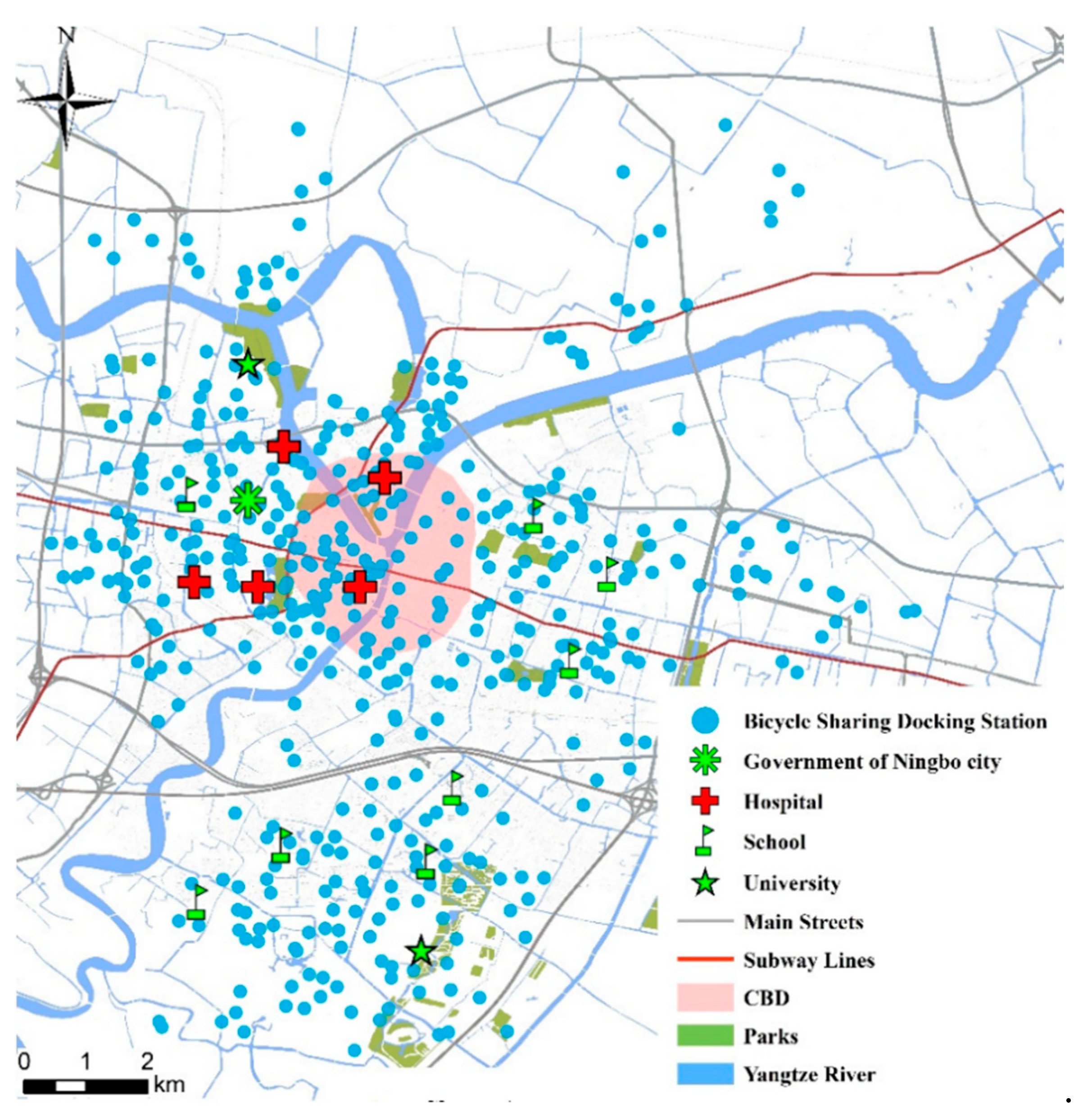
The study area of this paper is the central urban area of Ningbo, China. An automatic bicycle sharing system supported by information technology was officially put into operation in Ningbo city on 22 September 2013 [29]. In 2015, there were 477 bicycle sharing docking stations in the central urban area of Ningbo city. This system could obtain general mobility data through the origin-destination matrices associated with users’ and maintain the daily use of smart cards. Figure 1 shows the distribution of bicycle sharing docking stations in Ningbo city.
3.2. Smart Card Data of Bicycle Sharing System
Smart card data used in this paper was provided by Ningbo Bicycle Sharing System. Key information stored in the smart card data includes latitude and longitude of each station, smart card ID, rental time, return time, station ID. Data used in this paper include 17 days of smart card data from 10 May to 26 May 2015.
A preprocessing data cleansing procedure was used to take away those smart card records with incorrect or useless transaction information. Smart card data was removed if it showed the following characteristics: Rides with return time before rental time, which indicates a potential error of the information system; data from stations with only a few records, which may show non-typical usage patterns and thus distort the clustering result [30]; although Yahya [31] detected detailed usage patterns of bicycle sharing without deleting the short time duration records, we removed the rides that showed trip duration less than 1 min as Vogel, Greiser and Mattfeld [30] and Xu, et al. [32] did. They suggested that if a bicycle was immediately returned after being picked up, an actual ride did not take place.
3.3. POI Data around Bicycle Sharing Docking Station
Point of interest (POI), a new type of electronic map data of land use, which generally includes four parts of information: name, type, geographical coordinates, and address. Nowadays, there is more and more research on land use characteristics using this new type of data. POI data can quantify the precise land use characteristics, and it can be extracted from an electronic map. This paper uses POI data to reveal the influence of different land use type on a bicycle sharing system.
According to the information provided by the website of the Ningbo Bicycle Sharing System, the average distance of bicycle sharing docking stations was approximately 400 m [29], therefore the half of average distance (200 m) is the average attractive radius of the Ningbo Bicycle Sharing System [28]. In order to explore the influence of land use characteristics on bicycle sharing docking stations, all POI data of land use characteristics were extracted within 200 m of bicycle sharing docking stations from the electronic map. POI data were extracted from Baidu map [33], which is classified into 13 primary categories and more than 100 secondary categories, and all the secondary categories will be merged into the primary level [34]. Thirteen primary categories include Catering, Hotel, Shopping, Living Service, Tourist Sites, Leisure and Entertainment, Education, Medical, Traffic Facilities, Financial Institutions, Real Estate, Corporations, and Government Institutions.
4. Methodology
The methodology of this paper will be introduced in three parts: method of clustering algorithms, description of temporal variables and description of spatial variables.
4.1. Clustering Algorithms and Clustering Validation Measures
This paper applied three clustering algorithms: Hierarchical clustering, k-means clustering, and expectation-maximization (EM) clustering. Hierarchical clustering is one of the broadly-used unsupervised statistical methods that classify items into some hierarchy of clusters (groups) based on their similarities [35]. Agglomerative and hierarchical, this clustering algorithm makes a tree structure emerge with adjoining branches forming between similar groups which can be cut at a chosen height to produce the desired number of clusters. Each observation is originally placed as its unique cluster. Then the clusters are successively merged together based on the most similarity of their paring. For the pairing of any two clusters, it is decided by a dissimilarity matrix and can be based on various agglomeration methods.
An iterative method, k-means algorithm is the most fundamental and most useful algorithm for clustering [36]. For a given number of clusters, it can minimize the within-class sum of squares [37]. Its efficiency to a great extent relies on the choice of the cluster centers. When the algorithm starts, random procedures are applied to create starting clustering centers, then each observation is put in its closest cluster. Therefore, the cluster centers are updated, and the entire process is repeated, finally, objects are relocated by minimizing the distances of objects within clusters and maximizing the distance of objects in different clusters.
A model-based clustering, EM clustering functions with a Gaussian mixture model. This model is extended from the k-means algorithm [38]. K-means only takes into account the distance to the closest cluster when assigning points to clusters. Yet EM clustering also computes the probability that a point belongs to a cluster. As the probability depends on both the distance from the cluster center and the spread (variance) of the cluster, a point that is closer to the centroid of one cluster than another may well become more likely to belong to the latter cluster if it has a much higher spread [38].
Methods that display the connectedness, compactness, and separation of the cluster partitions are adopted for internal validation. Connectedness reflects what extent observations are put in the same cluster as those closest to them in the data space and is here measured by the connectivity [39]. The connectivity measured that observations are put in the same cluster as those closest to them in the data space [39]. Ranging between zero and infinity, its value declines more and the clustering shows better. Compactness assesses cluster homogeneity, usually by looking at the intra-cluster variance, while separation quantiles the degree of separation between clusters [40]. The Dunn index [41] and silhouette width [42] were selected for examples of non-linear combinations of the compactness and separation. Ranging between zero and infinity, the value of the Dunn index should be higher for a better result. The same is with the value of the silhouette width that ranges from −1 to 1.
For the stability validation, we selected the average proportion of non-overlap (APN), the average distance (AD) and the average distance between means (ADM) [43]. They serve to compare the results from full data-based clustering to clustering based on the removal of each column, one at a time. The stability measures will function particularly well with highly-correlated data, a case that is quite normal with high-throughput genomic data [40]. All stability measures with values close to zero correspond to highly-consistent clustering results, which indicates a less value is better for clustering.
According to internal measures and stability measures, we can conclude the most suitable cluster method and an optimal number of clusters for our research.
4.2. Temporal Variables
Splitting stations according to the sum number of pickups and returns can be easily affected by population density, geographical location, and other factors. Therefore, the usage pattern of the whole system is broken down to every station recording pickups and returns activities on an hourly basis. This can reflect the different usage patterns in different course of the day at different stations [30]. The activity at station level is defined by the ratio of pickups or returns: the number of pickups or returns in a certain hour divided by the total pickup or return number of the day. In doing so, 48 temporal attribute variables that depict the daily pickups and returns of every station are obtained.
4.3. Spatial Variables
In previous research, it is difficult to depict the influence of land use characteristics on a bicycle sharing system. The GWR model can effectively investigate the spatial variability of land use characteristics in traffic demand research [44]. We extracted all POI data (13 types) around bicycle sharing docking stations of the Ningbo Bicycle Sharing System, and built a GWR model of returns and pickups of the bicycle sharing system. Each bicycle sharing docking station has its own parameter estimates and t-statistic value from the GWR model. Then, we got 26 spatial attribute variables describing the effect of land use characteristics on daily pickups and returns of every station.
4.3.1. GWR Model
A GWR model has been proposed to address the spatial heterogeneity problem when modeling spatially aggregated data. Especially, some early studies have used GWR models to identify the spatial interaction between regional industrialization level and other factors [45], to explore the spatial patterns of both crime and its covariates [46] and to understand the relationships between urban vibrancy and land-use configurations [47]. We used the GWR model to quantify the influence of different POIs on bicycle sharing usage.
The spatial autocorrelation test should be applied firstly. By using spatial autocorrelation techniques, we can explore whether or not the daily return and pick up changes are spatially correlated to the geographical coordinates of bicycle sharing docking stations [48]. Moran’s I statistic is a spatial autocorrelation statistic that can be used for measuring spatial dependency [49]. The calculation formula of global Moran’s I is shown in Equation (1) [49].
where n is spatial sample size, and are observed value of sample and , is a spatial relationship between sample and , when sample and are closed, otherwise . The range of index of global Moran’s I is [−1, 1].
Software GWR 4.0 is often used to calculate the Moran’s I index value and z-score and p-value to evaluate the significance of the Index [50]. P-values are numerical approximations of the area under the curve for a known distribution, limited by the test statistic. The spatial pattern of the variable is clustered when z-score is significantly greater than zero; it is dispersed when z-score is significantly less than zero, and it is random when z-score is significantly close to zero [48].
If variables pass the spatial autocorrelation test, the GWR model can be applied. The traditional global ordinary least squares (OLS) model will be explored before using the GWR model to make sure there is no multicollinearity among variables [51]. The variance inflation factor (VIF), which indicates the severity of the multicollinearity, is computed when the OLS analysis is completed. The variable with VIF higher than 10 should be deleted [49].
The GWR model is extended from the global ordinary linear regression model. The geographical coordinate data are embedded in the samples and make the model realize local regression. The expression of GWR model is shown in Equation (2) [52].
where i (i = 1, 2, …, n) denotes a bicycle sharing station; are the coordinates of station i; is the dependent variable of station i; is the kth explanatory variable; is the error term for station i; represents the intercept; is the regression coefficient.
In contrast to the OLS model in which parameter estimation is fixed for each observation, the distinct characteristic of GWR model is that coefficient varies across the model to measure the spatial variations of observations.
Every sample has its own local regression model. In the GWR model, it can be determined by a kernel weighting scheme. In Ningbo city, the bicycle sharing docking station is denser in the center of the study area and sparser in the periphery of the study area. Therefore, the adaptive Gaussian kernel weighting scheme is applied in this GWR model [53]. The optimal bandwidth is determined by the corresponding value that results in the minimum corrected Akaike information criterion (AICc) [54]. The performance of the local model, as compared to the global model, can be identified through the adjusted R-squared value and corrected Akaike information criterion (AICc). A model with a larger adjusted R-squared and lower AICc represents a better goodness of fit. The GWR 4.0 software was used to estimate parameters of the GWR models.
4.3.2. Inputs of GWR Model
As Wu, Inhi and Hyungchul [34] and Calvo, et al. [55] suggested, we chose average daily returns and pickups of each bicycle sharing docking station as the dependent variable of the GWR model. The number of average daily returns and pickups is extracted from smartcard data including 10 weekdays from 10 May to 23 May 2014. The calculation formula of average daily returns and pickups of docking stations is shown in Equation (3).
The explanatory variable of the GWR model is POI data close to bicycle sharing docking stations in Ningbo city. All variables and their descriptions are summarized in Table 1.
4.3.3. Output of the GWR Model
Results of the Moran I test show that all z-scores of POI variables are significantly (p-values < 0.05) and that the spatial pattern of POI variables is clustered (high values cluster near other high values; low values cluster near other low values). Therefore, the spatial variability is proved to exist in all POI variables, and it’s reasonable to apply the GWR model in this research.
Considering spatial variability of POI variables, the GWR model is calibrated here with an adaptive Gaussian kernel weighting scheme. Each bicycle sharing docking station has its own parameter estimates and t-statistic value from GWR model. Some POI variables have insignificant parameters (|t-statistic| < 1.96) in some docking stations, which indicates that this type of POI variable has no significant influence on returns or pickups in these docking stations. In order to conform to the actual situation, we modified these insignificant estimated parameters as zero to represent no significant influence on bicycle sharing docking station. The final significant estimated parameters of the GWR model is shown in Table 2. Negative values of estimated coefficients in Table 2 mean that the variables have negative effects on the dependent variable, while positive values represent positive effects.
The OLS model must be calibrated first so as to explore the global influence of POI variables on bicycle sharing demand and to avoid the multicollinearity among variables. Table 2 indicates that applying these POI variables will not produce multicollinearity (VIF < 10). Compared with OLS model, GWR model has larger Adj. R-square and lesser AICc (Adj. R-square (GWR) = 0.497 > Adj. R-square (OLS) = 0.308; AICc (GWR) = 6231 < AICc (OLS) = 6381), which indicates that GWR model has a better performance than OLS model.
As Table 2 shows, most of the POI variables have significant positive impacts on returns and pickups, and the influence of POI variables is varying in different bicycle sharing docking stations. According to the median of estimated parameters, the POI variables can be divided into two groups. The first group includes Catering, Shopping, Education, Traffic Facilities, Financial Institutions, Real Estate, and Corporations. These POI variables have a great influence on returns and pickups (median > 10) because the trips of these POI variables are either the daily travel of citizens (like Catering, Shopping, and Traffic Facilities) or commuting travel of workers and students (like Corporations, Real Estate and Education). Many bicycle sharing docking stations are set for these trip purposes. The second group includes Hotel, Living Service, Tourist Site, Leisure and Entertainment, Medical, and Government Institution. These POI variables have a smaller influence on returns and pickups (median < 10) because the trips of these POI variables are not necessary trips on weekdays for travelers.
The estimated parameters of the GWR model indicate the precise influence parameters of different types of land use characteristics on bicycle sharing usage and they provide a better understanding of spatial variability of land use characteristics. From the outputs of the GWR model, we obtained 26 (13 for returns, 13 for pickups) spatial variables of land use characteristic for every bicycle sharing docking station.
5. Results of Clustering
Hierarchical, K-means and EM clustering is applied to the normalized spatial variables and temporal variables for a number of clusters varying from two to twenty. Through R package clValid, the top four ranking cluster algorithms for each measure are given in Table 3.
It is clear that K-means with seven clusters yields the best result on four of the six measures. Thus, it is easy for us to select the overall winner in this case. The bicycle sharing docking stations of Ningbo city are clustered for seven clusters by K-means clustering. Stations were grouped in seven clusters according to their spatiotemporal activities with the help of the K-means clustering algorithm.
For a better spatiotemporal analysis of the obtained clusters, Table 4 illustrates the most influential POI (s) and usage peak hour period(s) for every cluster.
As shown in Table 4, the Corporations and Financial Institutions POIs have great influence on bicycle sharing returns and pickups of Cluster 1. As most stations of cluster 1 are located close to the center of the study area, which is CBD of Ningbo city, they were around financial centers with business departments and organizations. The ratio of pickup and return activities during the peak period (7:00–9:00 and 17:00–19:00) was much higher, reaching 50% of the total number. Yet these activities were quite rare or even none during other time of the day. Thus, it was considered to serve only the commuting during the peak period.
For cluster 2, the Real Estate and Shopping POIs have great influence. This cluster of stations is located around residential places, which presents a high residential density. Due to the communities, it was obvious that pickup activity was very active in morning peak periods (7:00–9:00) for work. In evening peak periods (17:00–19:00), people went home from work, thus making the return activity more active than any other time in the day. Apart from commuting, residents in the communities also went out for life purposes. Thus, there was an obvious increase of the return activity from 8:00–10:00 in the morning when people came home from market places and also an increase of pickup activity between 19:00–20:00 when people went out for recreational activities.
Most stations of cluster 3 are located around the several commercial districts of Ningbo city. These commercial districts are full of restaurants and stores, a strong attraction for people living here. The catering and shopping POIs have a great influence on cluster 3. This kind of stations has three peaks every weekday. The first one is the morning peak from 7:00–9:00. This may be because the staff of commercial districts would go to work at that time. The second peak is around noon from 11:00–14:00. This may be because people cycle to restaurants for lunch; the third peak is evening peak periods form 17:00–20:00. This may be because many Chinese people like shopping and eating in commercial districts after work.
The Education and Catering POIs have a great influence on cluster 4. Stations of cluster 4 tend to be located around primary and high schools. Therefore, this kind of stations is laid for students and parents who pick up their children. Stations of cluster 4 have four peaks every weekday, which correspond to school attendance and departure respectively in the forenoon and in the afternoon. Stations of cluster 5 have an obvious attribute of traffic facilities. They are mainly around subway stations and other traffic hubs, serving primarily for traffic transfer. Therefore, no obvious peak activities were seen from 7:00 to 19:00, but they were busy throughout the day time. The Government Institutions and Medical POIs have a great influence on bicycle sharing returns and pickups of cluster 6. Stations of cluster 6 tend to be located around public management and service utilities such as administrative departments and hospitals of Ningbo city. Commuting was the main reason for morning peaks (7.00–9.00) when people went to work while pickup activities were centered on evening peak (17.00–19.00) when people went home from work. Except commuting, during other time of the day, there were only some certain activities, which may be because people need to conduct affairs or go to the hospital by public bicycles. The last cluster is mainly surrounded by entertainment places and tourist sites where pickup and return activities were well-distributed during the day. Yet both pickup and return activities particularly increase between 17:00 and 20:00, reflecting that many more people came out to have fun during the time.
6. Conclusions
This paper explored the spatiotemporal activities pattern in the Ningbo Bicycle Sharing System, China through the analysis of smart card data and POI data. Through preprocessing smart card data cleansing procedure, we get the proportion of pickup and return activities of each station as temporal attributes variables. By applying POI data and building a GWR model, we get spatial attribute variables describing the effect of land use characteristics on pickup and return activities of each bicycle sharing station.
According to the performance of the three clustering algorithms and six cluster validation measures, the 477 bicycle sharing docking stations are clustered into seven clusters by K-means clustering. Through analysis, each cluster has its unique temporal activities and is influenced by comprehensive land use characteristics. Pickup and return activities were quite different among the seven clusters, which were caused by people’s travel habits and land use characteristics around stations. This study provides a better understanding of the spatiotemporal activities pattern of bicycle sharing system in Ningbo city and assists investors and business owners in selecting locations and designing stations for better operation and management of a bicycle sharing system.
This study could be extended by considering more factors such as weather, weekends and holidays when using clustering. Notably, taking the average daily returns and pickups as the dependent variables will reduce the variation of the data. More research on the hourly bicycle sharing usage pattern is thus suggested. Additionally, borrowing and returning bicycle behavior within a short time period (e.g., 60 s) may have two situations: a real short ride or just checking the bicycle without using it. The identification of such behavior can provide a reference in the preprocessing phase. Finally, further study on the relationship between dockless bicycle sharing systems and docked bicycle sharing systems and the interaction of shared bicycle usage and transit use are also needed.
Author Contributions
Conceptualization, R.C.; Data curation, Y.J. and X.M.; Formal analysis, Y.J. and X.M.; Methodology, R.C.; Revision, X.M.
Funding
This research was funded by the International Cooperation and Exchange of the National Natural Science Foundation of China, grant number 51561135003, the Key Project of National Natural Science Foundation of China, grant number 51338003, and the Scientific Research Foundation of Graduated School of Southeast University, grant number YBPJ1882.
Conflicts of Interest
The authors declare no conflict of interest.
References
- Maizlish, N.; Woodcock, J.; Co, S.; Ostro, B.; Fanai, A.; Fairley, D. Health Cobenefits and Transportation-Related Reductions in Greenhouse Gas Emissions in the San Francisco Bay Area. Am. J. Public Health 2013, 103, 703–709. [Google Scholar] [CrossRef] [Green Version]
- Yang, M.; Liu, X.; Wang, W.; Li, Z.; Zhao, J. Empirical Analysis of a Mode Shift to Using Public Bicycles to Access the Suburban Metro: Survey of Nanjing, China. J. Urban Plan. Dev. 2016, 142, 05015011. [Google Scholar] [CrossRef]
- Meddin, R.; Demaio, P.J. The Bike-Sharing World Map. Available online: www.bikesharingmap.com (accessed on 27 February 2019).
- Yang Fang, M.G. Report of Shared Bicycle. Available online: http://tech.sina.com.cn/roll/2018-03-07/doc-ifxtevrp244313 (accessed on 27 February 2019).
- Tang, Y.; Pan, H.; Shen, Q. Bike-sharing systems in Beijing, Shanghai, and Hangzhou and their impact on travel behavior (No. 11-3862). In Proceedings of the Transportation Research Board 90th Annual Meeting, Washington, DC, USA, 23–27 January 2011. [Google Scholar]
- Shaheen, S.A.; Zhang, H.; Martin, E.; Guzman, S. China’s Hangzhou Public Bicycle. Transp. Res. Record J. Transp. Res. Board 2011, 2247, 33–41. [Google Scholar] [CrossRef]
- Fishman, E.; Washington, S.; Haworth, N. Bike Share: A Synthesis of the Literature. Urban Transp. China 2013, 33, 148–165. [Google Scholar] [CrossRef] [Green Version]
- Industry, T.I.o.C. The Information of China Industry, The Analysis of History, Status Quo and Scale of China’s Public Bicycle in 2017. Available online: http://www.chyxx.com/industry/201704/513812.html (accessed on 27 February 2019).
- GuangZhou Planning Bureau. The Case of Big Data Combined with City Planning. Available online: https://mp.weixin.qq.com/s?__biz=MzA3OTU3ODgxNA==&mid=2650583825&idx=1&sn=4a1e2f4df6d96e0d08ba639278f1da8e&chksm=87b940c0b0cec9d65ee7a76a0d25232d7811a83ab3858052d019bfb98780669aed6d4ed67139&mpshare=1&scene=23&srcid=0628YETa2Iyklv5UMuD51Exy#rd (accessed on 27 February 2019).
- Du, M.; Cheng, L. Better Understanding the Characteristics and Influential Factors of Different Travel Patterns in Free-Floating Bike Sharing: Evidence from Nanjing, China. Sustainability 2018, 10, 1244. [Google Scholar] [CrossRef]
- Transportation, D.O. Guidance to Encourage and Regulate Bike Sharing Was Issued. Available online: http://www.gov.cn/xinwen/2017-08/03/content_5215640.htm (accessed on 27 February 2019).
- Nikitas, A. Understanding bike-sharing acceptability and expected usage patterns in the context of a small city novel to the concept: A story of ‘Greek Drama’. Transp. Res. Part F Traffic Psychol. Behav. 2018, 56, 306–321. [Google Scholar] [CrossRef]
- Froehlich, J.E.; Neumann, J.; Oliver, N. Sensing and predicting the pulse of the city through shared bicycling. In Proceedings of the Twenty-First International Joint Conference on Artificial Intelligence, Pasadena, CA, USA, 17 July 2009. [Google Scholar]
- De Chardon, C.M.; Caruso, G.; Thomas, I. Bike-share rebalancing strategies, patterns, and purpose. J. Transp. Geogr. 2016, 55, 22–39. [Google Scholar] [CrossRef]
- Fishman, E. Bikeshare: A Review of Recent Literature. Transp. Rev. 2016, 36, 92–113. [Google Scholar] [CrossRef]
- Shaheen, S.A.; Cohen, A.P.; Martin, E.W. Public Bikesharing in North America: Early Operator Understanding and Emerging Trends. Transp. Res. Rec. J. Transp. Res. Board 2013, 1568, 83–92. [Google Scholar] [CrossRef]
- Ricci, M. Bike sharing: A review of evidence on impacts and processes of implementation and operation. Res. Transp. Bus. Manag. 2015, 15, 28–38. [Google Scholar] [CrossRef] [Green Version]
- Zhang, Y. Survey on the reorganization and using status of public bicycle system in urban fringe areas: Taking Tongzhou and Daxing Districts of Beijing for example. Urban Probl. 2015, 3, 42–46. [Google Scholar]
- Fishman, E.; Washington, S.; Haworth, N. Erratum to Bike share: A synthesis of the literature (Transport Reviews). Transp. Rev. 2013, 33. [Google Scholar] [CrossRef]
- Kaltenbrunner, A.; Meza, R.; Grivolla, J.; Codina, J.; Banchs, R. Urban cycles and mobility patterns: Exploring and predicting trends in a bicycle-based public transport system. Pervasive Mob. Comput. 2010, 6, 455–466. [Google Scholar] [CrossRef]
- Rahul, T.M.; Verma, A. A study of acceptable trip distances using walking and cycling in Bangalore. J. Transp. Geogr. 2014, 38, 106–113. [Google Scholar] [CrossRef]
- Zhao, J.; Wang, J.; Deng, W. Exploring bikesharing travel time and trip chain by gender and day of the week. Transp. Res. Part C 2015, 58, 251–264. [Google Scholar] [CrossRef]
- Li, X.; Zhang, Y.; Zhang, R.; Lu, Y.; Xie, S. Overcoming Barriers to Cycling: Exploring Influence Factors of Cyclists’ Preference in Free-Floating Bikesharing; Technical Report No. 18-02707; The National Academies of Sciences, Engineering, and Medicine: Washington, DC, USA, 8 January 2018. [Google Scholar]
- Mauri, C. Card loyalty. A new emerging issue in grocery retailing. J. Retail. Consum. Serv. 2003, 10, 13–25. [Google Scholar] [CrossRef]
- Borgnat, P.; Abry, P.; Flandrin, P.; Robardet, C.; Rouquier, J.-B.; Fleury, E. Shared bicycles in a city: A signal processing and data analysis perspective. Adv. Complex Syst. 2011, 14, 415–438. [Google Scholar] [CrossRef]
- Come, E.; Randriamanamihaga, N.A.; Oukhellou, L.; Aknin, P. Spatio-temporal analysis of dynamic origin-destination data using latent dirichlet allocation: Application to vélib’bike sharing system of paris. In Proceedings of the TRB 93rd Annual Meeting, Washington, DC, USA, 12–16 January 2014; p. 19. [Google Scholar]
- Austwick, M.Z.; O’Brien, O.; Strano, E.; Viana, M. The structure of spatial networks and communities in bicycle sharing systems. PLoS ONE 2013, 8, e74685. [Google Scholar]
- O’brien, O.; Cheshire, J.; Batty, M. Mining bicycle sharing data for generating insights into sustainable transport systems. J. Transp. Geogr. 2014, 34, 262–273. [Google Scholar] [CrossRef]
- System, C.o.N.B.S. Ningbo Public Bicycle Service Development Co. Operational Information. Available online: http://www.nbbicycle.com (accessed on 27 February 2019).
- Vogel, P.; Greiser, T.; Mattfeld, D.C. Understanding bike-sharing systems using data mining: Exploring activity patterns. Procedia-Soc. Behav. Sci. 2011, 20, 514–523. [Google Scholar] [CrossRef]
- Yahya, B. Overall bike effectiveness as a sustainability metric for bike sharing systems. Sustainability 2017, 9, 2070. [Google Scholar] [CrossRef]
- Xu, C.; Wang, Y.; Wang, C.; Liu, P. Investigation of Contributing Factors to Travel Demand of Free-floating Bike Sharing: A Geographically Weighted Regression Approach (No. 19-03556). In Proceedings of the Transportation Research Board 98th Annual Meeting, Washington, DC, USA, 13–17 January 2019. [Google Scholar]
- Corporation, B. Classification of Poi Data. Available online: http://lbsyun.baidu.com/index.php?title=lbscloud/poitags (accessed on 27 February 2019).
- Wu, C.; Inhi, K.; Hyungchul, C. A geographically weighted regression model to explore the relationship between built 1 environment and public sharing bike flow: Evidence from Suzhou, China. In Proceedings of the TRB 98th Annual Meeting, Washington, DC, USA, 13–17 January 2019. [Google Scholar]
- Ward, J.H., Jr. Hierarchical grouping to optimize an objective function. J. Am. Stat. Assoc. 1963, 58, 236–244. [Google Scholar] [CrossRef]
- Teboulle, M.; Berkhin, P.; Dhillon, I.; Guan, Y.; Kogan, J. Clustering with Entropy-Like K-Means Algorithms; Springer: Berlin/Heidelberg, Germany, 2006. [Google Scholar]
- Hartigan, J.A.; Wong, M.A. Algorithm AS 136: A K-Means Clustering Algorithm. J. R. Stat. Soc. 1979, 28, 100–108. [Google Scholar] [CrossRef]
- Tan, P.N. Introduction to Data Mining; Pearson Education India: Noida, India, 2018; Available online: https://www-users.cs.umn.edu/~kumar001/dmbook/sol.pdf (accessed on 27 February 2019).
- Handl, J.; Knowles, J.; Kell, D.B. Computational cluster validation in post-genomic data analysis. Bioinformatics 2005, 21, 3201–3212. [Google Scholar] [CrossRef] [PubMed] [Green Version]
- Brock, G.; Pihur, V.; Datta, S.; Datta, S. clValid, an R package for cluster validation. J. Stat. Softw. 2011. Available online: https://cran.microsoft.com/web/packages/clValid/vignettes/clValid.pdf (accessed on 27 February 2019).
- Dunn, J.C. Well separated clusters and fuzzy partitions. J. Cybern. 1974, 4, 95–104. [Google Scholar] [CrossRef]
- Rousseeuw, P.J. Silhouettes: A graphical aid to the interpretation and validation of cluster analysis. J. Comput. Appl. Math. 1987, 20, 53–65. [Google Scholar] [CrossRef] [Green Version]
- Datta, S.; Datta, S. Comparisons and validation of statistical clustering techniques for microarray gene expression data. Bioinformatics 2003, 19, 459–466. [Google Scholar] [CrossRef] [Green Version]
- Brunsdon, C.; Fotheringham, S.; Charlton, M. Geographically weighted regression. J. R. Stat. Soc. Ser. D 1998, 47, 431–443. [Google Scholar] [CrossRef]
- Huang, Y.; Leung, Y. Analysing regional industrialisation in Jiangsu province using geographically weighted regression. J. Geogr. Syst. 2002, 4, 233–249. [Google Scholar] [CrossRef]
- Cahill, M.; Mulligan, G. Using geographically weighted regression to explore local crime patterns. Soc. Sci. Comput. Rev. 2007, 25, 174–193. [Google Scholar] [CrossRef]
- Wu, C.; Ye, X.; Ren, F.; Du, Q. Check-in behaviour and spatio-temporal vibrancy: An exploratory analysis in Shenzhen, China. Cities 2018, 77, 104–116. [Google Scholar] [CrossRef]
- Bebber, D. Spatial autocorrelations. Trends Ecol. Evol. 1999, 14, 196. [Google Scholar] [CrossRef]
- Bao, J.; Liu, P.; Yu, H.; Xu, C. Incorporating twitter-based human activity information in spatial analysis of crashes in urban areas. Accid. Anal. Prev. 2017, 106, 358–369. [Google Scholar] [CrossRef]
- Getis, A.; Ord, J.K. The Analysis of Spatial Association by Use of Distance Statistics. Geogr. Anal. 1992, 24, 189–206. [Google Scholar] [CrossRef]
- Charlton, M.; Fotheringham, A. Geographically Weighted Regression (White Paper). National Centre for Geocomputation National University of Ireland, Maynooth. GWR_WhitePaper. pdf 2009. Available online: https://www.geos.ed.ac.uk/~gisteac/fspat/gwr/gwr_arcgis/GWR_WhitePaper.pdf (accessed on 27 February 2019).
- Brunsdon, C.; Fotheringham, A.S.; Charlton, M.E. Geographically weighted regression: A method for exploring spatial nonstationarity. Geogr. Anal. 1996, 28, 281–298. [Google Scholar] [CrossRef]
- Qian, X.; Ukkusuri, S.V. Spatial variation of the urban taxi ridership using GPS data. Appl. Geogr. 2015, 59, 31–42. [Google Scholar] [CrossRef]
- Mcmillen, D.P. Geographically Weighted Regression: The Analysis of Spatially Varying Relationships. Am. J. Agric. Econ. 2004, 86, 554–556. [Google Scholar] [CrossRef]
- Calvo, F.; Eboli, L.; Forciniti, C.; Mazzulla, G. Factors influencing trip generation on metro system in Madrid (Spain). Transp. Res. Part D Transp. Environ. 2019, 67, 156–172. [Google Scholar] [CrossRef]
Figure 1.
Bicycle sharing docking stations of Ningbo city.


Table 1.
Summary and descriptive statistics of variables of the GWR model.
| Variable | Description | Unit | Source | Mean |
|---|---|---|---|---|
| Dependent Variable | ||||
| ADR | Average daily returns of each bicycle sharing docking station | Trips/day | Smartcard | 173.87 |
| ADP | Average daily pickups of each bicycle sharing docking station | 175.56 | ||
| Explanatory Variable | ||||
| Catering | Total number of 13 types of POI data around bicycle sharing docking station | Number of POI | Electronic Map | 21.33 |
| Hotel | 2.71 | |||
| Shopping | 13.23 | |||
| Living Service | 13.55 | |||
| Tourist Sites | 3.14 | |||
| Leisure & Entertainment | 2.46 | |||
| Education | 1.52 | |||
| Medical | 1.59 | |||
| Traffic Facilities | 3.08 | |||
| Financial Institutions | 3.26 | |||
| Real Estate | 5.43 | |||
| Corporations | 16.94 | |||
| Government Institution | 4.18 | |||
Table 2.
Estimated results of the GWR model.
| Returns | Pickups | ||||||
| Variables | Lower Quartile | Median | Upper Quartile | Lower Quartile | Median | Upper Quartile | VIF |
| Catering | 6.569 | 12.946 | 18.367 | 11.519 | 19.741 | 26.735 | 3.88 |
| Hotel | 1.010 | 3.547 | 5.798 | 1.588 | 3.967 | 6.399 | 3.74 |
| Shopping | 22.442 | 30.306 | 37.345 | 22.181 | 31.112 | 38.640 | 1.99 |
| Living Service | 3.578 | 5.768 | 9.346 | 3.157 | 8.707 | 9.296 | 1.42 |
| Tourist Sites | 1.644 | 7.873 | 12.121 | 2.282 | 5.142 | 9.476 | 1.58 |
| Leisure & Entertainment | −0.290 | 2.256 | 6.950 | −0.575 | 2.116 | 6.250 | 4.14 |
| Education | 5.370 | 16.331 | 21.590 | 5.043 | 16.809 | 20.277 | 1.10 |
| Medical | −0.164 | 2.603 | 6.065 | 0.169 | 2.901 | 6.439 | 4.33 |
| Traffic Facilities | 4.796 | 10.926 | 17.607 | 4.407 | 10.225 | 17.089 | 1.25 |
| Financial Institutions | 4.141 | 11.804 | 18.530 | 3.984 | 12.025 | 18.477 | 4.22 |
| Real Estate | 8.502 | 12.482 | 17.145 | 8.765 | 13.110 | 17.331 | 2.36 |
| Corporations | 3.469 | 11.114 | 20.388 | 2.944 | 12.955 | 17.292 | 1.26 |
| Government Institution | 3.140 | 5.136 | 8.935 | 2.174 | 4.174 | 8.442 | 3.15 |
| CONSTANT | 169.831 | 184.617 | 197.535 | 169.705 | 185.525 | 199.314 | - |
| Result of GWR Model | Result of OLS Model | ||||||
| Number of samples | 477 | Number of samples | 477 | ||||
| Adj. R-square | 0.497 | Adj. R-square | 0.308 | ||||
| AICC | 6231 | AICC | 6381 | ||||
Table 3.
Optimal comparison results of the clustering algorithm.
| 1 | 2 | 3 | 4 | |
|---|---|---|---|---|
| Connectivity | Hierarchical-2 | Hierarchical-7 | Kmeans-2 | Kmeans-3 |
| Dunn | Kmeans-7 | Kmeans-15 | Kmeans-16 | Kmeans-18 |
| Silhouette | Kmeans-7 | Kmeans-8 | Kmeans-2 | EM-3 |
| APN | Kmeans-7 | Kmeans-8 | Hierarchical-3 | Hierarchical-19 |
| AD | EM-20 | EM-19 | EM-18 | EM-17 |
| ADM | Kmeans-7 | Kmeans-9 | Hierarchical-3 | EM-4 |
Table 4.
Most significant POI (s) and usage peak hour period(s) for each Cluster.
| Stations of Each Cluster | Clusters | Most Significant POI (s) | Usage Peak Hour Period(s) |
|---|---|---|---|
| 138 | Cluster 1 (Pickups) | Corporations, Financial Institutions | 7:00–9:00, 17:00–19:00 |
| Cluster 1 (Returns) | Corporations, Financial Institutions | 7:00–9:00, 17:00–19:00 | |
| 58 | Cluster 2 (Pickups) | Real Estate, Shopping | 7:00–9:00, 19:00–20:00 |
| Cluster 2 (Returns) | Real Estate, Shopping | 8:00–10:00, 17:00–19:00 | |
| 74 | Cluster 3 (Pickups) | Catering, Shopping | 7:00–9:00, 11:00–14:00, 17:00–20:00 |
| Cluster 3 (Returns) | Catering, Shopping | 7:00–9:00, 11:00–14:00, 17:00–20:00 | |
| 27 | Cluster 4 (Pickups) | Education, Catering | 7:00–9:00,13:00–14:00 |
| Cluster 4 (Returns) | Education, Catering | 11:00–12:00, 17:00–19:00 | |
| 45 | Cluster 5 (Pickups) | Traffic Facilities | 7:00–19:00 |
| Cluster 5 (Returns) | Traffic Facilities | 7:00–19:00 | |
| 70 | Cluster 6 (Pickups) | Government Institution, Medical | 7:00–9:00 |
| Cluster 6 (Returns) | Government Institution, Medical | 17:00–19:00 | |
| 65 | Cluster 7 (Pickups) | Leisure & Entertainment, Tourist Sites | 17:00–20:00 |
| Cluster 7 (Returns) | Leisure & Entertainment, Tourist Sites | 17:00–20:00 |
© 2019 by the authors. Licensee MDPI, Basel, Switzerland. This article is an open access article distributed under the terms and conditions of the Creative Commons Attribution (CC BY) license (http://creativecommons.org/licenses/by/4.0/).
Share and Cite
MDPI and ACS Style
Ma, X.; Cao, R.; Jin, Y. Spatiotemporal Clustering Analysis of Bicycle Sharing System with Data Mining Approach. Information 2019, 10, 163. https://0-doi-org.brum.beds.ac.uk/10.3390/info10050163
AMA Style
Ma X, Cao R, Jin Y. Spatiotemporal Clustering Analysis of Bicycle Sharing System with Data Mining Approach. Information. 2019; 10(5):163. https://0-doi-org.brum.beds.ac.uk/10.3390/info10050163
Chicago/Turabian StyleMa, Xinwei, Ruiming Cao, and Yuchuan Jin. 2019. "Spatiotemporal Clustering Analysis of Bicycle Sharing System with Data Mining Approach" Information 10, no. 5: 163. https://0-doi-org.brum.beds.ac.uk/10.3390/info10050163
Note that from the first issue of 2016, this journal uses article numbers instead of page numbers. See further details here.