Impact of Information Sharing and Forecast Combination on Fast-Moving-Consumer-Goods Demand Forecast Accuracy

Abstract

This article empirically demonstrates the impacts of truthfully sharing forecast information and using forecast combinations in a fast-moving-consumer-goods (FMCG) supply chain. Although it is known a priori that sharing information improves the overall efficiency of a supply chain, information such as pricing or promotional strategy is often kept proprietary for competitive reasons. In this regard, it is herein shown that simply sharing the retail-level forecasts—this does not reveal the exact business strategy, due to the effect of omni-channel sales—yields nearly all the benefits of sharing all pertinent information that influences FMCG demand. In addition, various forecast combination methods are used to further stabilize the forecasts, in situations where multiple forecasting models are used during operation. In other words, it is shown that combining forecasts is less risky than “betting” on any component model.

1. Introduction

Demand forecasting at various forecast horizons is a key component in manufacturing operation management. Although the demand-forecasting problem have been addressed extensively in the literature and from many perspectives, the evolution of the complex supply chain—such as exposure to new data types, new retailing regimes, or new operation strategies—creates new challenges and opportunities for more accurate forecasts.

Forecast skill generally depends on two factors: the amount of data (information) that is available, and the depth of understanding about the underlying data-generating process. Whereas many papers in the literature focus on better inferring the underlying process, i.e., proposing various models to improve forecasts for a particular application, the integration of information across a supply chain is relatively less discussed. From an operational perspective, it is well understood that coordination across an entire supply chain creates win-win situations for all players in that supply chain. Such coordination is not just limited to the flow of materials, but also requires effective flow of information [1,2]. In a typical supply chain, the amount of demand-related data are abundant, ranging from a news release on a catastrophic event that may affect the global demand of a particular product, to a mobile-device advertising campaign launched by a local retailer. It is almost impossible for a particular player in a supply chain to obtain, manage, and use all of this information during forecasting. As a result, demand forecasts are often generated by using only an organization’s internal data. For example, a manufacturer usually produces forecasts based on historical order data; the accuracy of such forecasts is often limited. On this point, the first contribution of this paper is therefore on investigating the benefits of forecast information sharing in a supply chain.

Another challenge of the demand forecasting problem originates from the fact that the underlying data-generating processes may not be unique. Each entity in a supply chain may identify one or more appropriate models for their operational forecasts. To that end, two types of inconsistency are frequently encountered in supply-chain management: (1) the aggregation inconsistency across various levels in a supply chain, and (2) the inconsistency due to the multi-modeling of demand. The demand structure in a supply chain can be considered as a hierarchy, where goods produced by a manufacturer (top level) are shipped to its distributors, and, subsequently, retailers (bottom level). When the forecasts are produced by different supply-chain entities with different models, aggregation consistency is not guaranteed. In other words, the demand forecasts produced by different retailers do not add up exactly to the forecast produced by a manufacturer. The second type of inconsistency originates from the fact that, oftentimes, supply-chain entities use more than one model to generate forecasts. The question “to combine or not to combine?” has led to much debate over decades (e.g., [3,4,5]) since at least 1969, when Bates and Granger [6] published their seminal paper on forecast combination. The second contribution of this paper is therefore on addressing the forecast inconsistencies, in fast-moving-consumer-goods (FMCG) demand, through reconciliation and forecast combination.

2. Literature Review

The literature review is divided into four parts. A summary is presented at the end of the section to relate the various ideas herein discussed.

2.1. On Information Sharing

Although it is known a priori that more information—provided that it is relevant—leads to better forecasts, the supply-chain literature on this topic seems to be divided. On one hand, with no surprise, there are abundant papers in the literature, many being empirical, showing that sharing historical demand information between downstream retailers and upstream suppliers is valuable. On the other hand, a stream of research says that, under certain conditions, sharing of demand information from downstream retailers to upstream suppliers is not valuable, as the historical time series data of the retailers’ orders provides sufficient information for suppliers to impute the end-consumer demand process. In other words, the divided insights are partially subject to whether the retailer-level demand is inferable from the retailers’ order data (see [7,8] and references therein for more details).

In a recent study, Ali and Boylan [9] showed that the part of literature that supports “no value of information sharing” mostly relies on certain restrictive assumptions, some of which may not hold in practice. For example, Cui et al. [10] showed that there is indeed value in sharing the demand time series. Although they use a similar demand-process model as papers showing “no value of information sharing”, they find that, when retailers change their inventory policy (contingent on some private information), sharing the demand time series is valuable for the supply chain. The reader is referred to [10,11] for further information on such debate.

Apart from the general debate on information sharing, there are also more focused works on forecast sharing in supply chain (e.g., [12,13,14,15]). These works are mostly theoretical and/or dealing with supply-chain contracting. For instance, the authors in [13,14] considered a scenario where the retailer may game the system by strategically distorting the shared information. The game-theoretic interaction between retailers and suppliers, i.e., the continuum between the “all-or-nothing” cooperation (The term “all-or-nothing” is used to describe the situations where the supply-chain members either absolutely trust each other and cooperate or do not trust each other at all.) was modeled. Nevertheless, such behavior can be argued away by invoking the Folk theorem—a class of theorems about possible Nash equilibrium payoff profiles in repeated games [16]. Even when the interactions are not long-term, truthful sharing of forecasts can be encouraged by using appropriately designed contracts [15]. To that end, this paper assumes that all shared forecasts are truthful. Based on this assumption, this paper, along with the aforementioned papers, provides a strong prescription for supply-chain managers: sharing forecast information truthfully provides most of the benefits derived by sharing more (potentially sensitive) details, such as pricing or promotional strategies.

2.2. On Forecast Reconciliation

The concept of reconciliation emerges when the forecast quantity, such as renewable power generation [17,18,19], electrical load [20], tourism demand [21], or FMCG demand [22], can be modeled as a hierarchy. Due to the different information sets available at various levels in the hierarchy, e.g., retailers’ business strategy is opaque to the distributor, and modeling uncertainties, the lower-level forecasts almost surely do not sum up to the higher-level forecasts. When such aggregation inconsistency is observed, decision makers are challenged with a selection problem, i.e., which set of forecasts should be used? In the case of FMCG forecasting, such inconsistency contradicts the core idea of manufacturing operation management, namely, effective and efficient supply–demand matching.

In the literature, there are several well-known aggregate-consistent forecasting methods, such as the bottom-up approach, top-down approach, or middle-out approach [21]. Bottom-up approach assumes the forecasts at a higher level of the hierarchy are the arithmetic sum of the bottom-level forecasts. In this case, a manufacturer does not make its own forecasts but awaits retailers’ forecasts (sometimes in the form of order data). However, due to the need of creating “safety stock”, retailers often over-forecast their demand. The excess demand propagates up the supply chain and results in a phenomenon commonly known as the bullwhip effect [23,24], which leads to inefficiency in supply chain. Another aggregate-consistent forecasting method is the top-down approach, which assumes the forecasts of lower-level demand are fractions of the manufacturer’s total forecast. There are several ways to assign such fractions. However, such demand assignment often leads to inventory shortage/excess at lower levels. The middle-out approach combines the previous two approaches by initiating forecast from a middle level of the demand hierarchy; the forecasts on other levels are aggregated or disaggregated using the middle-level forecasts. However, when the supply chain is complex and contains many levels, identifying the “middle-level player” is not trivial; it also involves contracting issues that may complicate operation.

Recently, through a series of papers [21,25,26,27], the optimal reconciliation technique—as detailed in the next section—was demonstrated. This technique takes the independently-made forecasts at various levels in a hierarchy (also known as the base forecasts), and produces a set of aggregate-consistent forecasts. Since the base forecasts are generated by different supply-chain entities, most likely using the best information available to these entities, they are often more accurate. Furthermore, as only the forecasts are required, neither the forecasting model nor the raw data needs to be revealed to the other entities. Due to the omni-channel sales, even when a particular forecast shows an increase in demand, the specific business strategy that causes that boost remains opaque to the peers, and thus protects the supply-chain entity who made that forecast. There are several versions of optimal reconciliation; this paper does not consider all of them. Instead, the aim is to demonstrate the benefits of forecast sharing, and thus only one version is used to exemplify the reconciliation procedure.

2.3. On Forecast Combination

Twenty years after the paper by Bates and Granger [6], Granger [28] noted in his review that the combination of forecasts is a simple, pragmatic, and sensible way to possibly produce better forecasts. Forecast combination often works even when some component forecasts are inefficient. For such reasons, forecast combination has become a standard practice in many scientific domains (e.g., [29,30,31]).

The core idea of forecast combination is to produce a final forecast using several component forecasts. Supposing N component forecasts, ${\widehat{y}}_t^{(i)}$, $i\in \{1,\cdots ,N\}$, are available, the combine forecast takes the form:

$$\begin{array}{cc}\hfill {\widehat{y}}_t^{(c)}=& {\alpha }_0+\sum _{i=1}^N{\alpha }_i{\widehat{y}}_t^{(i)},\hfill \end{array}$$

(1)

where ${\alpha }_i$ are the weights placed on the component forecasts. It is immediately clear that there are many ways to estimate those weights. de Menezes et al. [32] summarized seven well-established methods that were thought to be good representatives of varying degrees of sophistication. The reader is referred to the original paper for details. Among the seven methods discussed by de Menezes et al. [32], the regression-based combination has the most variants. This paper considers several popular methods including ordinary least squares, least absolute deviations, lasso, and complete subset regression.

2.4. On FMCG Forecasting

FMCG demand forecasting, or any other forecasting, is essentially an input–output matching problem, where the input is the historical and current information, and the output is the forecast. To construct an appropriate forecasting model, many methods are available. For instance, econometric approaches (e.g., [33,34]) and machine-learning approaches (e.g., [35]) have both been used in the demand forecasting literature. The reader is referred to the work by Fildes et al. [36] for a comprehensive review on forecasting in operation research. In the supply-chain-planning process, due to the large number of factors that may affect demand, forecasting is often done in two steps. An automated forecasting system would produce an initial demand forecast and some adjustments are made subsequently based on either an expert’s view, or some other algorithms [37].

General-purpose univariate forecasting methods, such as the autoregressive integrated moving average (ARIMA) family of models, or the exponential smoothing (ETS) family of models, are available in many statistical software packages, such as R or Python. They are therefore commonly utilized by the industry. Since forecasts that consider domain knowledge (exogenous factors) are generally better than those solely relying on univariate modeling, the output of a univariate forecasting method can be further adjusted using domain knowledge. For example, the base-times-lift model [38] is one such model.

Besides postprocessing the forecasts, the exogenous information can also be built into the forecasting models directly. In the case of FMCG demand forecasting, Huang et al. [39] considered the autoregressive distributed lag (ADL) model, which had shown excellent performance for their dataset. A large number of exogenous variables, as well as the lagged version of these variables, were used in their ADL model. The model is quite general and customizable. The complete form of the model is given by:

$$\begin{array}{cc}ln(y_{0,t})=\hfill & {\alpha }_0+\sum _{j=1}^{\ell }{\alpha }_{j}ln(y_{0,t-j})+\sum _{j=0}^{{\ell }^{\prime }}{\beta }_{0,j}ln(p_{0,t-j})+\sum _{j=0}^{{\ell }^{″}}{\gamma }_{0,j}{\mathcal{I}}_{0,t-j}+\sum _{p=1}^P\sum _{j=0}^{{\ell }^{*}}{\beta }_{p,j}ln(p_{p,t-j})\hfill \\ & +\sum _{q=1}^Q\sum _{j=0}^{{\ell }^{**}}{\gamma }_{q,j}{\mathcal{I}}_{q,t-j}+\sum _{d=1}^{12}{\theta }_d{\mathrm{monthly}\_\mathrm{dummy}}_d+\sum _{c=1}^9\sum _{\nu =0}^1{\delta }_{c,\nu }{\mathrm{calendar}\_\mathrm{event}}_{c,t-\nu }+{\epsilon }_t,\hfill \end{array}$$

(2)

where $y_0$ is the demand of the focal product; $p_0$ and $p_p$ are the price of the focal and competitor products; and ${\mathcal{I}}_0$ and ${\mathcal{I}}_q$ are the promotion index of the focal and competitor products. Together with the 12-month dummy variable and the dummy variables for nine major public holidays (and the weeks before that) in the US, if ${\ell }^{\prime }={\ell }^{″}={\ell }^{*}={\ell }^{**}=P=Q=2$, the model would have 48 exogenous variables. Huang et al. [39] showed that the ADL model not only outperforms the ETS and base-times-lift models, but also marginally outperformed the reduced (without competitor information) ADL model. However, only a reduced model is considered in this paper because the real-time information on pricing and promotional strategy, as well as the corresponding demand times series faced by the competitors, are seldom available in practice. Moreover, a reduced model is less likely to be over-specified as compared to the full model.

2.5. Section Summary

In view of the above literature review, the following aspects are discussed in the remaining part of the paper:

• Various information-sharing strategies in hierarchical FMCG demand forecasting. Four cases are elaborated, based on different levels of information sharing. Forecasting models are selected based on the available information in each case. More specifically, Case I (see below) considers univariate forecasting models (ARIMA and ETS); Case II considers a reduced ADL model; the forecasting models for Case III utilizes hierarchical reconciliation; and Case IV again uses the ADL model, but with more predictors.
• Hierarchical reconciliation procedure. It has three main steps: (1) arrange the data into a hierarchical structure, (2) generate base forecasts, and (3) reconcile the base forecasts. Two methods, namely, the bottom-up approach and the optimal reconciliation are used.
• Effect of combining forecasts. After the forecast accuracies under different levels of information sharing are compared, all models are subsequently treated as component models to investigate the effect of combining forecasts. A total of seven forecast combination methods are considered in this paper.

3. Cases of Different Levels of Information Sharing and Hierarchical Reconciliation

In this section, details of the supply-chain structure and the different cases of information sharing are elaborated. More specifically, four cases are considered: (1) no information other than the past demand is shared (Case I); (2) the past demand, price, and promotional information, i.e., all past pertinent information, is shared (Case II); (3) only the past demand time series and the retailers’ forecasts are shared (Case III); and (4) the past demand, price, and promotion time series, as well as the future planned pricing and promotional campaign strategies, are shared (Case IV).

Obviously, these cases are arranged in an increasing order in terms of the amount of shared information. Case IV is the one where all pertinent information is shared, so naturally it is expected to perform the best. However, this case is highly unrealistic, as future price and promotional campaign strategies are highly-sensitive information that retailers may not be willing to share. Case II also comes with practical challenges, as it would require retailers to divulge their historical pricing and promotional strategies. However, one may argue that this information may be less sensitive than what is needed for Case IV. Case I, on the other hand, does not have any challenge in terms of feasibility, nevertheless, its forecast accuracy may be greatly limited by the lack of information. Finally, Case III comes with relatively fewer practical challenges than Cases II and IV; it is thus argued to be the most feasible case of information sharing in the retail industry.

Before the forecasting models for each case are revealed, the hierarchical nature of the supply chain is exemplified. The number of levels in a demand hierarchy and the aggregation/disaggregation interpretation may vary according to the granularity of the supply-chain structure. For example, one may either disaggregate the total demand based on product types or do so geographically. Without loss of generality, Figure 1 shows a three-level hierarchical demand time series structure, which will be used throughout this paper.

In Figure 1, the level 0 (${\mathcal{L}}_0$) demand is disaggregated based on n universal product codes (UPCs) to form the time series at level 1 (${\mathcal{L}}_1$). At ${\mathcal{L}}_1$, $y_{i,t}$ represents the demand of UPC i at time t. For each UPC, the demand is further disaggregated based on stores to form the level 2 (${\mathcal{L}}_2$) time series. Here, $y_{ij,t}$ represents the demand of UPC i at store j at time t. Let $m_i$ be the number of stores that sell UPC i, then the total number of ${\mathcal{L}}_2$ demand time series is ${\sum }_{i=1}^n{m}_i$.

3.1. Case I

Case I assumes that the business strategies of the downstream retailers are completely opaque to their supplier. In the context of Figure 1, it implies that the pricing and promotional strategies at ${\mathcal{L}}_2$ are unknown to ${\mathcal{L}}_0$ and ${\mathcal{L}}_1$. Under this setting, the information set at time t available to the supplier is

$$\begin{array}{c}\hfill {\Omega }_t^{\mathrm{I}}=\{{\mathit{Y}}_{{\mathcal{L}}_2,1},\cdots ,{\mathit{Y}}_{{\mathcal{L}}_2,t-1}\},\end{array}$$

(3)

where

$$\begin{array}{cc}\hfill {\mathit{Y}}_{{\mathcal{L}}_2,t^{\prime }}=& {\left(y_{11,t^{\prime }},\cdots ,y_{1m_1,t^{\prime }},\cdots ,y_{n1,t^{\prime }},\cdots ,y_{n{m}_n,t^{\prime }}\right)}^{\top },t^{\prime }\in \{1,\cdots ,t-1\}\hfill \end{array}$$

(4)

is the historical retailer-level demand.

Using ${\Omega }_t^{\mathrm{I}}$, the supplier can come up with a ${\mathcal{L}}_1$ forecast by first aggregating the demand data:

$$\begin{array}{cc}\hfill {\mathit{Y}}_{{\mathcal{L}}_1,t^{\prime }}=& {\left(\sum _{j=1}^{m_1}{y}_{1j,t^{\prime }},\cdots ,\sum _{j=1}^{m_n}{y}_{nj,t^{\prime }}\right)}^{\top }={\left(y_{1,t^{\prime }},\cdots ,y_{n,t^{\prime }}\right)}^{\top },t^{\prime }\in \{1,\cdots ,t-1\},\hfill \end{array}$$

(5)

so that the n UPC-level demand time series $\{y_{i,1},\cdots ,y_{i,t-1}\}$, $i\in \{1,\cdots ,n\}$, are obtained. Subsequently, univariate forecasting methods can be used on the aggregated time series. In this work, two frequently used univariate families of models are considered for Case I, namely, ARIMA and ETS. Furthermore, the case number and model abbreviation in SmallCaps are jointly used to denote a model, e.g., the ARIMA family of models for Case I is denoted as C1arima.

3.2. Case II

In this case, it is assumed that the retailers share the historical price, promotion, and the corresponding demand information with their supplier. Sharing such information does not pose severe practical challenges from an operational perspective. In fact, for those supply-chain relationships governed by long-term contracts, such information can be shared by enabling connectivity between IT systems of the firms. However, from a strategic perspective, retailers may not want to divulge their historical pricing and promotional strategy, since such information may be useful for their competitors in updating their priors. In other cases when the competitors also source from the same supplier, leakage of competitive information may not be ruled out completely. Therefore, this case poses certain strategic barriers to being implemented in practice.

The information set in this case is:

$$\begin{array}{c}\hfill {\Omega }_t^{\mathrm{II}}=\{{\mathit{Y}}_{{\mathcal{L}}_2,1},\cdots ,{\mathit{Y}}_{{\mathcal{L}}_2,t-1},{\mathcal{P}}_{{\mathcal{L}}_2,1},\cdots ,{\mathcal{P}}_{{\mathcal{L}}_2,t-1},{\mathcal{I}}_{{\mathcal{L}}_2,1},\cdots ,{\mathcal{I}}_{{\mathcal{L}}_2,t-1}\},\end{array}$$

(6)

where the additional terms to Case I, namely,

$$\begin{array}{cc}\hfill {\mathcal{P}}_{{\mathcal{L}}_2,t^{\prime }}=& {\left(p_{11,t^{\prime }},\cdots ,p_{1m_1,t^{\prime }},\cdots ,p_{n1,t^{\prime }},\cdots ,p_{n{m}_n,t^{\prime }}\right)}^{\top },t^{\prime }\in \{1,\cdots ,t-1\},\hfill \end{array}$$

(7)

$$\begin{array}{cc}\hfill {\mathcal{I}}_{{\mathcal{L}}_2,t^{\prime }}=& {\left({\mathcal{I}}_{11,t^{\prime }},\cdots ,{\mathcal{I}}_{1m_1,t^{\prime }},\cdots ,{\mathcal{I}}_{n1,t^{\prime }},\cdots ,{\mathcal{I}}_{n{m}_n,t^{\prime }}\right)}^{\top }\hfill \end{array}$$

(8)

are the historical retailer-level price and promotions information, respectively.

Whereas the ${\mathcal{L}}_1$ demand is the simple summation of the ${\mathcal{L}}_2$ demand (see Equation (5)), the ${\mathcal{L}}_1$ price and promotional information needs to be strategically aggregated. A weighted-average approach is used:

$$\begin{array}{cc}\hfill p_{i,t^{\prime }}=& \sum _{j=1}^{m_i}\left({\mathrm{ACV}}_j\times p_{ij,t^{\prime }}/\sum _{j=1}^{m_i}{\mathrm{ACV}}_j\right),t^{\prime }\in \{1,\cdots ,t-1\},\hfill \end{array}$$

(9)

$$\begin{array}{cc}\hfill {\mathcal{I}}_{i,t^{\prime }}=& \sum _{j=1}^{m_i}\left({\mathrm{ACV}}_j\times {\mathcal{I}}_{ij,t^{\prime }}/\sum _{j=1}^{m_i}{\mathrm{ACV}}_j\right),\hfill \end{array}$$

(10)

when aggregating ${\mathcal{P}}_{{\mathcal{L}}_2,t^{\prime }}$ and ${\mathcal{I}}_{{\mathcal{L}}_2,t^{\prime }}$. ${\mathrm{ACV}}_j$ is the all commodity volume (ACV) of retailer j, i.e., the annual sales volume of retailer j. Equations (9) and (10) average the price and promotion index of each retailer according to the store’s ACV. In other words, a bigger store receives a higher demand during a promotional campaign than a smaller store with the same promotion.

Considering the exogenous factors, the ${\mathcal{L}}_1$ forecasts for Case II can be produced via a regression model:

$$\begin{array}{cc}\hfill y_{i,t}=& exp\left[{\alpha }_0^{i,t}+\sum _{k=1}^{\ell }{\alpha }_k^{i,t}ln(y_{i,t-k})+\sum _{k=1}^{{\ell }^{\prime }}{\beta }_k^{i,t}ln(p_{i,t-k})+\sum _{k=1}^{{\ell }^{″}}{\gamma }_k^{i,t}{\mathcal{I}}_{i,t-k}+{\epsilon }_{i,t}\right],\hfill \end{array}$$

(11)

where $i\in \{1,\cdots ,n\}$ is the index set for the UPCs under consideration. Parameters ℓ, ${\ell }^{\prime }$, and ${\ell }^{″}$ control the numbers of lagged values of the dependent variable and each explanatory variable. The regression parameters in Equation (11), namely, ${\alpha }_0^{i,t}$, ${\alpha }_k^{i,t}$, ${\beta }_k^{i,t}$, and ${\gamma }_k^{i,t}$ are designed as adaptive parameters, to capture the changing dynamics in the demand series. After the regression parameters are estimated, the forecast for UPC i at time t is given by:

$$\begin{array}{cc}\hfill {\widehat{y}}_{i,t}=& exp\left[{\widehat{\alpha }}_0^{i,t}+\sum _{k=1}^{\ell }{\widehat{\alpha }}_k^{i,t}ln(y_{i,t-k})+\sum _{k=1}^{{\ell }^{\prime }}{\widehat{\beta }}_k^{i,t}ln(p_{i,t-k})+\sum _{k=1}^{{\ell }^{″}}{\widehat{\gamma }}_k^{i,t}{\mathcal{I}}_{i,t-k}\right].\hfill \end{array}$$

(12)

As parameter estimation is not the primary concern of this paper, least squares fitting is used throughout the text. Furthermore, the model equations (such as Equation (11)) and the prediction equations (such as Equation (12)) will be used interchangeably hereafter. In conclusion, a reduced form of the ADL model is used for Case II or C2adl.

3.3. Case III

Case III refers to a situation where retailers share their forecasts with their suppliers. Just like Cases I and II, it is assumed that the historical demand information is available to the supplier. However, the price and promotional information is assumed unknown to the supplier. The information available is thus ${\Omega }_t^{\mathrm{III}}=\{{\mathit{Y}}_{{\mathcal{L}}_2,1},\cdots ,{\mathit{Y}}_{{\mathcal{L}}_2,t-1},{\widehat{\mathit{Y}}}_{{\mathcal{L}}_2,t}\}$, where ${\widehat{\mathit{Y}}}_{{\mathcal{L}}_2,t}$ denotes the forecasts made by retailers for time t. As mentioned earlier, the information available in Case III may even be less sensitive than that in Case II, as information on price and promotions is only embedded in the forecasts implicitly. In other words, if the supplier observes an increase in the forecast demand, due to the lack of information on ${\mathcal{P}}_{{\mathcal{L}}_2,t}$ and ${\mathcal{I}}_{{\mathcal{L}}_2,t}$, there is, however, no way for the supplier to infer the cause (e.g., a target promotion or a simple price reduction) of the additional demand. The pricing and promotional strategies of retailers are thus (somewhat) protected.

At first glance, Case III is straightforward, as the forecasts at ${\mathcal{L}}_1$ can be easily obtained by summing up ${\widehat{\mathit{Y}}}_{{\mathcal{L}}_2,t}$. However, doing so implies that the supplier is not utilizing the information provided by $\{{\mathit{Y}}_{{\mathcal{L}}_2,1},\cdots ,{\mathit{Y}}_{{\mathcal{L}}_2,t-1}\}$. Therefore, a more holistic approach is needed. A highlight of this paper is to present the usefulness of the optimal hierarchical reconciliation method [21,25] in forecasting for a supplier in a supply chain with multiple retailers.

In hierarchical reconciliation, simply summing up ${\widehat{\mathit{Y}}}_{{\mathcal{L}}_2,t}$ is referred to as the bottom-up approach. The reconciled forecasts at all levels, ${\tilde{\mathit{Y}}}_t$, using the bottom-up approach is:

$$\begin{array}{cc}\hfill {\tilde{\mathit{Y}}}_t=& \mathit{S}{\widehat{\mathit{Y}}}_{{\mathcal{L}}_2,t},\hfill \end{array}$$

(13)

where ${\widehat{\mathit{Y}}}_{{\mathcal{L}}_2,t}$ is given in Equation (22) below, and each entry therein is a forecast of a particular UPC at a particular store. $\mathit{S}$ is a summing matrix. For illustration purposes, consider Figure 1 with $n=3$, $m_i=3$, $i\in \{1,2,3\}$, and the summing matrix is given by:

$$\begin{array}{cc}\hfill \mathit{S}=& \left(\begin{array}{ccccccccc}1& 1& 1& 1& 1& 1& 1& 1& 1\\ 1& 1& 1& 0& 0& 0& 0& 0& 0\\ 0& 0& 0& 1& 1& 1& 0& 0& 0\\ 0& 0& 0& 0& 0& 0& 1& 1& 1\\ 1& 0& 0& 0& 0& 0& 0& 0& 0\\ 0& 1& 0& 0& 0& 0& 0& 0& 0\\ 0& 0& 1& 0& 0& 0& 0& 0& 0\\ 0& 0& 0& 1& 0& 0& 0& 0& 0\\ 0& 0& 0& 0& 1& 0& 0& 0& 0\\ 0& 0& 0& 0& 0& 1& 0& 0& 0\\ 0& 0& 0& 0& 0& 0& 1& 0& 0\\ 0& 0& 0& 0& 0& 0& 0& 1& 0\\ 0& 0& 0& 0& 0& 0& 0& 0& 1\end{array}\right).\hfill \end{array}$$

(14)

By observing the summing matrix, it becomes apparent how ${\tilde{\mathit{Y}}}_t$ may be obtained. For example, multiplying the second row of $\mathit{S}$ with ${\widehat{\mathit{Y}}}_{{\mathcal{L}}_2,t}$ gives the forecast for $y_{1,t}$.

The optimal reconciliation method is similar to the bottom-up approach, but it utilizes the information that is ignored by the bottom-up approach, namely, $\{{\mathit{Y}}_{{\mathcal{L}}_2,1},\cdots ,{\mathit{Y}}_{{\mathcal{L}}_2,t-1}\}$. The idea of optimal reconciliation originates from a linear regression model:

$$\begin{array}{cc}\hfill {\widehat{\mathit{Y}}}_t=& \mathit{S}{\mathbf{\beta }}_t+{\mathbf{ϵ}}_t,\hfill \end{array}$$

(15)

where ${\widehat{\mathit{Y}}}_t$ given by Equation (21) is a vector of all base forecasts, ${\mathbf{ϵ}}_t$ has zero mean and unknown covariance $\mathbf{\Sigma }$, and ${\mathbf{\beta }}_t=\mathbb{E}({\widehat{\mathit{Y}}}_{{\mathcal{L}}_2,t})$ is the unknown mean of retailer-level forecasts. As compared to Equation (13), Equation (15) models the errors associated with reconciliation (${\mathbf{ϵ}}_t$ should not be confused with the base-forecast errors). In other words, when the base forecasts are generated individually at ${\mathcal{L}}_0$, ${\mathcal{L}}_1$ and ${\mathcal{L}}_2$, Equation (15) explains the aggregate inconsistency in the forecasts.

Regression parameter ${\mathbf{\beta }}_t$ can be estimated using the generalized least squares (GLS):

$$\begin{array}{cc}\hfill {\widehat{\mathbf{\beta }}}_t^{\mathrm{GLS}}=& {({\mathit{S}}^{\top }{\mathbf{\Sigma }}^{†}\mathit{S})}^{-1}{\mathit{S}}^{\top }{\mathbf{\Sigma }}^{†}{\widehat{\mathit{Y}}}_t,\hfill \end{array}$$

(16)

where ${\mathbf{\Sigma }}^{†}$ is the Moore–Penrose generalized inverse of $\mathbf{\Sigma }$. A problem with the GLS solution is that the covariance matrix, $\mathbf{\Sigma }$, is unknown. As the length of ${\mathbf{ϵ}}_t$ is $l=1+n+{\sum }_{i=1}^n{m}_i$, i.e., the total number of base forecasts, there are $l(l+1)/2$ unknown parameters in $\mathbf{\Sigma }$ that need to be estimated. This is not a straightforward computation. Therefore, an alternative strategy is to use the weighted least squares (WLS) approach:

$$\begin{array}{cc}\hfill {\widehat{\mathbf{\beta }}}_t^{\mathrm{WLS}}=& {({\mathit{S}}^{\top }\mathbf{\Lambda }\mathit{S})}^{-1}{\mathit{S}}^{\top }\mathbf{\Lambda }{\widehat{\mathit{Y}}}_t,\hfill \end{array}$$

(17)

where $\mathbf{\Lambda }$ is a diagonal matrix whose elements are the inverse of the variances of ${\mathbf{ϵ}}_t$. Using the WLS solution, the optimally reconciled forecasts are:

$$\begin{array}{cc}\hfill {\tilde{\mathit{Y}}}_t=& \mathit{S}{\widehat{\mathbf{\beta }}}_t^{\mathrm{WLS}}=\mathit{S}{({\mathit{S}}^{\top }\mathbf{\Lambda }\mathit{S})}^{-1}{\mathit{S}}^{\top }\mathbf{\Lambda }{\widehat{\mathit{Y}}}_t.\hfill \end{array}$$

(18)

Using the optimal reconciliation technique, the entire information set ${\Omega }_t^{\mathrm{III}}$ is used. The results are thus expected to be better than those from a bottom-up approach. The following system of equations summarizes the forecast method in Case III:

$$\begin{array}{cc}\hfill {\tilde{\mathit{Y}}}_t=& \mathit{S}\mathit{P}{\widehat{\mathit{Y}}}_t;\hfill \end{array}$$

(19)

$$\begin{array}{cc}\hfill \mathit{P}=& {({\mathit{S}}^{\top }\mathbf{\Lambda }\mathit{S})}^{-1}{\mathit{S}}^{\top }\mathbf{\Lambda };\hfill \end{array}$$

(20)

$$\begin{array}{cc}\hfill {\widehat{\mathit{Y}}}_t=& {\left({\widehat{Y}}_{{\mathcal{L}}_0,t},{\widehat{\mathit{Y}}}_{{\mathcal{L}}_1,t}^{\top },{\widehat{\mathit{Y}}}_{{\mathcal{L}}_2,t}^{\top }\right)}^{\top };\hfill \end{array}$$

(21)

$$\begin{array}{cc}\hfill {\widehat{\mathit{Y}}}_{{\mathcal{L}}_2,t}=& {\left({\widehat{y}}_{11,t},\cdots ,{\widehat{y}}_{1m_1,t},\cdots ,{\widehat{y}}_{n1,t},\cdots ,{\widehat{y}}_{n{m}_n,t}\right)}^{\top };\hfill \end{array}$$

(22)

$$\begin{array}{cc}\hfill {\widehat{y}}_{ij,t}=& exp\left[{\widehat{\alpha }}_0^{ij,t}+\sum _{k=1}^{\ell }{\widehat{\alpha }}_k^{ij,t}ln(y_{ij,t-k})+\sum _{k=0}^{{\ell }^{\prime }}{\widehat{\beta }}_k^{ij,t}ln(p_{ij,t-k})+\sum _{k=0}^{{\ell }^{″}}{\widehat{\gamma }}_k^{ij,t}{\mathcal{I}}_{ij,t-k}\right],\hfill \\ \hfill & \mathrm{where}i\in \{1,\cdots ,n\},j\in \{1,\cdots ,m_i\};\hfill \end{array}$$

(23)

$$\begin{array}{cc}\hfill {\widehat{\mathit{Y}}}_{{\mathcal{L}}_1,t}=& {\left({\widehat{y}}_{1,t},\cdots ,{\widehat{y}}_{n,t}\right)}^{\top };\hfill \end{array}$$

(24)

$$\begin{array}{cc}\hfill {\widehat{y}}_{i,t}=& exp\left[{\widehat{\alpha }}_0^{i,t}+\sum _{k=1}^{\ell }{\widehat{\alpha }}_k^{i,t}ln(y_{i,t-k})\right];\hfill \end{array}$$

(25)

$$\begin{array}{cc}\hfill {\widehat{Y}}_{{\mathcal{L}}_0,t}=& exp\left[{\widehat{\alpha }}_0^t+\sum _{k=1}^{\ell }{\widehat{\alpha }}_k^{t}ln(y_{t-k})\right].\hfill \end{array}$$

(26)

Equation (19) is the general form of forecast reconciliation [21]. The bottom-up approach can be represented by setting $\mathit{P}$ as $({\mathbf{0}}_{m\times (n+1)}|{\mathit{I}}_m)$, where $\mathbf{0}$ and $\mathit{I}$ are null matrix and identity matrix respectively, $m={\sum }_{i=1}^n{m}_i$. Equation (23) produces ${\mathcal{L}}_2$ base forecasts. It assumes that the retailers know their own price and promotional information at a future time t; the summations over p and $\mathcal{I}$ thus start from $k=0$. Equations (25) and (26) produce ${\mathcal{L}}_1$ and ${\mathcal{L}}_0$ base forecasts, respectively. Regression parameters ${\alpha }_0^{ij,t}$, ${\alpha }_k^{ij,t}$, ${\beta }_k^{ij,t}$, ${\gamma }_k^{ij,t}$, ${\alpha }_0^{i,t}$, ${\alpha }_k^{i,t}$, ${\alpha }_0^t$ and ${\alpha }_k^t$ can be estimated using historical data via the least squares method. The bottom-up and optimal reconciliation techniques are hereafter denoted as, C3bu and C3opt, respectively.

3.4. Case IV

This case represents the ideal case for traditional supply-chain management. In this case, the retailers share all pertinent information with the supplier that is ${\Omega }_t^{\mathrm{IV}}=\{{\mathit{Y}}_{{\mathcal{L}}_2,1},\cdots ,{\mathit{Y}}_{{\mathcal{L}}_2,t-1},{\mathcal{P}}_{{\mathcal{L}}_2,1},\cdots ,{\mathcal{P}}_{{\mathcal{L}}_2,t},{\mathcal{I}}_{{\mathcal{L}}_2,1},\cdots ,{\mathcal{I}}_{{\mathcal{L}}_2,t}\}$. It is important to note that, in this case, different from Case II, the planned pricing and promotional strategy ${\mathcal{P}}_{{\mathcal{L}}_2,t}$ and ${\mathcal{I}}_{{\mathcal{L}}_2,t}$ are also shared. Due to the competitive importance of this information, this case is less practical than all other cases.

The forecast method for Case IV is identical to Case II except now that the planned price and promotional information for time t is available to the supplier:

$$\begin{array}{cc}\hfill {\widehat{y}}_{i,t}=& exp\left[{\widehat{\alpha }}_0^{i,t}+\sum _{k=1}^{\ell }{\widehat{\alpha }}_k^{i,t}ln(y_{i,t-k})+\sum _{k=0}^{{\ell }^{\prime }}{\widehat{\beta }}_k^{i,t}ln(p_{i,t-k})+\sum _{k=0}^{{\ell }^{″}}{\widehat{\gamma }}_k^{i,t}{\mathcal{I}}_{i,t-k}\right].\hfill \end{array}$$

(27)

${\mathcal{L}}_1$ price and promotion are aggregated through Equations (9) and (10), but for $t^{\prime }\in \{1,\cdots ,t\}$. This model is denoted as C4adl.

4. Forecast Combination Methods

Section 3 has discussed the various modeling approaches to be used in cases of different levels of information sharing. It is noted that there is information overlap among these cases. For example, suppose the information set ${\Omega }_t^{\mathrm{III}}$ is available, all forecasts in Case I also become available, i.e., ${\Omega }_t^{\mathrm{I}}\subset {\Omega }_t^{\mathrm{III}}$. Although it can be argued that the “best” method known to a forecaster will most likely outperform all other alternatives, e.g., C3opt will outperform C1arima, suboptimal forecasts sometimes can contribute positively to the final forecast, as discussed in Section 2. To that end, several frequently used forecast combination methods are formulated in this section.

4.1. Simple Averaging

The most intuitive way to combine forecasts is to use the average of all forecasts as the final combined forecast. Suppose a total of N component models are used to produce forecasts at each time stamp t, the final forecast is given by

$$\begin{array}{cc}\hfill {\widehat{y}}_t^{(\mathrm{avg})}=& \frac{1}{N}\sum _{i=1}^N{\widehat{y}}_t^{(i)},\hfill \end{array}$$

(28)

where ${\widehat{y}}_t^{(i)}$ is the forecast produced by method i, and ${\widehat{y}}_t^{(\mathrm{avg})}$ is the combined forecast using simple averaging. This method is denoted as Avg.

4.2. Trimmed Simple Averaging

In practice, if more than five component forecasts are available, the forecaster can afford to drop the highest and lowest forecasts, i.e., the outliers among the component forecasts. This method is known as the trimmed simple averaging, or Trim.

4.3. Combination through Variance

Avg puts equal weights on the component models. However, it can be argued that a heavier weight should be placed on a better performing model. The variance-based method (Var) computes the mean squared error (MSE) and weighs the forecasts according to their accuracy. Mathematically, it is expressed as:

$$\begin{array}{cc}\hfill {\widehat{y}}_t^{(\mathrm{var})}& =\sum _{i=1}^N\frac{\frac{1}{{\mathrm{MSE}}_i}}{{\sum }_{i=1}^N\frac{1}{{\mathrm{MSE}}_i}}{\widehat{y}}_t^{(i)}.\hfill \end{array}$$

(29)

It is noted that, in this method, some historical forecasts need to be available for the computation of MSE.

4.4. Combination through Ordinary Least Squares

Besides assigning equal or variance-based weights, another class of weight-assignment methods is through linear regression:

$$\begin{array}{cc}\hfill y_{t^{\prime }}=& {\mathit{x}}_{t^{\prime }}^{\top }\mathit{W}+e_{t^{\prime }},\hfill \end{array}$$

(30)

where ${\mathit{x}}_{t^{\prime }}={\left(1,{\widehat{y}}_{t^{\prime }}^{(1)},\cdots ,{\widehat{y}}_{t^{\prime }}^{(N)}\right)}^{\top }$ is the size-$(N+1)$ vector of component model forecasts at time $t^{\prime }$, $y_{t^{\prime }}$ is the actual demand at time $t^{\prime }$, and $\mathit{W}$ is the size-$(N+1)$ vector of weights. The above regression equation can be written into a vector form, if a total of T historical forecasts are available:

$$\begin{array}{cc}\hfill \mathit{Y}=& \mathit{X}\mathit{W}+\mathit{e},\hfill \end{array}$$

(31)

where $\mathit{Y}={\left(y_1,\cdots ,y_T\right)}^{\top }$, $\mathit{e}={\left(e_1,\cdots ,e_T\right)}^{\top }$, and

$$\begin{array}{cc}\hfill \mathit{X}=& \left(\begin{array}{c}{\mathit{x}}_1^{\top }\\ ⋮\\ {\mathit{x}}_T^{\top }\end{array}\right)=\left(\begin{array}{cccc}1& {\widehat{y}}_1^{(1)}& \cdots & {\widehat{y}}_1^{(N)}\\ ⋮& ⋮& \ddots & ⋮\\ 1& {\widehat{y}}_T^{(1)}& \cdots & {\widehat{y}}_T^{(N)}\end{array}\right).\hfill \end{array}$$

(32)

If the weight vector $\mathit{W}$ can be estimated, the combined forecast at time t can be obtained via

$$\begin{array}{cc}\hfill {\widehat{y}}_t=& {\mathit{x}}_t^{\top }\widehat{\mathit{W}}.\hfill \end{array}$$

(33)

Given the regression setting, the ordinary least squares (OLS) method provides a basic solution to $\mathit{W}$:

$$\begin{array}{cc}\hfill {\widehat{\mathit{W}}}^{\mathrm{OLS}}=& {({\mathit{X}}^{\top }\mathit{X})}^{-1}{\mathit{X}}^{\top }\mathit{Y}.\hfill \end{array}$$

(34)

This method is denoted as Ols.

4.5. Combination through Least Absolute Deviations

Whereas the OLS regression minimizes ${\sum }_{t^{\prime }=1}^T{(e_{t^{\prime }})}^2$, the median regression, or least absolute deviations (LAD) regression, minimizes ${\sum }_{t^{\prime }=1}^T\left|e_{t^{\prime }}\right|$, i.e.,

$$\begin{array}{cc}\hfill {\widehat{\mathit{W}}}^{\mathrm{LAD}}=& \underset{\mathit{W}}{error}\left\{\sum _{t^{\prime }=1}^T\left|y_{t^{\prime }}-{\mathit{x}}_{t^{\prime }}^{\top }\mathit{W}\right|\right\}.\hfill \end{array}$$

(35)

Linear programming is required to solve for ${\mathit{W}}^{\mathrm{LAD}}$. The advantage of LAD is that it treats all samples equally, whereas OLS penalizes the large errors. In other words, LAD is more resistant to outliers in the component forecasts.

4.6. Combination through Lasso

Similarly, lasso is another commonly used regression technique, which minimizes the sum of squares subject to a regularization on the $L_1$ norm of the regression parameter. Formally, the lasso estimator is given by:

$$\begin{array}{cc}\hfill {\widehat{\mathit{W}}}^{\mathrm{lasso}}=& \underset{\mathit{W}}{error}\left\{\sum _{t^{\prime }=1}^T{\left(y_{t^{\prime }}-w_0-\sum _{i=1}^N{\widehat{y}}_{t^{\prime }}^{(i)}{w}_i\right)}^2+\lambda \sum _{i=1}^N\left|w_i\right|\right\}.\hfill \end{array}$$

(36)

Due to its geometry, see Tibshirani [40], lasso is capable of shrinking some regression parameters to zero, and thus acts as a variable selection method. In the present context, lasso shrinks and selects only the good component model forecasts, which may be more appropriate than OLS and LAD.

4.7. Combination through Complete Subset Regression

The last variant of the regression-based combination method considered in this paper is the complete subset regression. Given N component models, a total of $\Psi$ regressions can be built, where

$$\begin{array}{cc}\hfill \Psi & =\sum _{i=1}^N\left(\begin{array}{c}N\\ i\end{array}\right)=\sum _{i=1}^N\frac{N!}{i!(N-1)!}.\hfill \end{array}$$

(37)

These $\Psi$ combined forecasts can then be combined for a final forecast using averaging—mean, median, mode, or any other combination method. This method is denoted as Subset.

5. Empirical Study

The empirical part of this paper considers the FMCG data from a retail chain. The data are stored in the Dominick’s database (http://research.chicagobooth.edu/kilts/marketing-databases/dominicks/), which is freely available online. The dataset is provided by the James M. Kilts Center, University of Chicago Booth School of Business with a collaborative effort by the Dominick’s Finer Food (DFF). Although the dataset records weekly historical data from 1989 to 1994, owing to its informative nature, it is still frequently being used to conduct marketing research (e.g., [41,42]). It was previously found that sales promotions in Dominick’s database are large and frequent [43]; the dataset thus provides a suitable platform for our current investigation, i.e., forecasting under strong demand fluctuation.

The database contains four types of files: the customer count file, store-level demographics file, UPC files, and movement files. Store-level sales information for FMCG from 29 categories, along with the store-level price and promotional information, is provided in the movement files. Since the goal of this paper is to investigate the benefits of information sharing during forecasting, only data from one category, namely, the bottled juice category (BJC), is used. However, similar results and conclusions can be expected, should the data from other categories be used.

There are three types of promotion in BJC: simple price reduction, bonus buy, and coupons, with bonus buy being the dominant type (e.g., three bottles of cranberry juice for 10 dollars). As the price in the data file is registered for the bundle, the total price is simply divided by the size of the bundle to obtain the price of a single item (which is equivalent to a price reduction). In addition, a “1” is recorded if a particular store has a promotion (any type) on a particular product. After careful data preprocessing and filtering (e.g., list-wise deletion of missing values), complete data from 37 UPCs over a period of 377 weeks remain. These UPCs are listed in the first column of

Table 1. Universal product code (UPC) level mean absolute percentage errors for the bottled juice category. The colored columns 3–8 compare forecast accuracies under different levels of information sharing, i.e., Cases I–IV. The combined forecasts using various methods are displayed in columns 9–15.

		Component Models						Combined Forecasts
UPC	$\mathit{n}.{\mathcal{L}}_{\mathbf{2}}$	C1ets	C1arima	C2adl	C3bu	C3opt	C4adl	Avg	Trim	Var	Ols	Lad	Lasso	Subset
7045011402	55	10.97	10.88	9.44	7.48	6.97	7.77	7.35	7.23	7.19	6.73	8.13	6.87	6.85
5300015154	61	9.58	9.51	9.49	9.24	9.06	9.33	8.76	8.74	8.77	9.46	8.94	9.12	9.08
5300015108	64	13.10	14.02	11.83	10.39	10.41	11.71	11.40	11.02	11.35	11.85	10.57	11.61	12.08
3828103123	61	17.06	17.33	16.53	20.13	19.42	17.15	15.36	15.43	15.68	12.37	11.85	12.32	13.51
3828103091	66	38.12	40.32	34.03	22.21	22.20	27.46	27.78	26.96	26.42	29.16	18.85	26.48	27.77
3828103025	52	57.05	52.18	24.51	18.13	17.72	17.10	24.59	20.54	22.23	48.04	16.13	46.25	30.65
3828103021	63	113.02	211.64	53.78	35.91	35.62	37.02	72.00	47.21	50.81	47.75	40.71	52.98	44.78
3120027407	42	29.46	36.50	28.61	17.94	18.09	12.47	21.27	20.07	17.25	13.23	10.61	13.23	13.61
3120027007	53	26.89	32.80	29.31	12.35	12.48	13.24	18.35	17.24	13.66	13.98	12.22	17.15	14.20
3120026134	52	26.42	24.26	24.79	11.33	11.49	12.68	16.42	15.45	13.09	11.94	11.91	12.09	11.81
3120021007	62	26.42	29.21	21.93	12.08	12.05	10.62	15.12	14.10	11.56	12.25	11.01	23.78	12.74
3120020035	63	22.45	22.91	19.61	8.99	8.94	9.01	12.91	11.99	9.88	9.16	9.60	14.28	9.14
3120020007	65	32.73	28.84	21.33	10.56	10.43	9.56	14.66	12.73	10.52	17.65	15.78	18.26	15.64
3120020005	66	54.05	52.50	32.74	11.26	11.36	11.92	26.33	23.57	16.96	15.55	14.36	39.36	12.18
1480031656	65	75.89	58.68	33.14	22.87	22.90	22.76	30.83	25.69	27.78	30.98	28.83	27.16	28.71
1480000034	67	84.17	73.04	39.76	27.50	27.96	28.71	38.12	34.39	30.93	36.07	24.96	33.80	38.29
7045011328	61	10.81	11.59	12.45	11.20	10.77	8.31	9.54	9.26	9.24	9.04	8.76	8.36	8.66
5300015132	66	15.13	16.72	15.47	17.82	16.73	18.55	14.85	14.40	14.99	14.33	14.15	14.76	14.39
4850000193	34	29.11	29.52	25.98	13.01	13.06	13.46	18.34	17.28	15.70	14.90	12.03	12.26	13.61
4180022700	54	10.46	10.91	10.06	16.01	14.86	9.65	10.59	10.36	9.98	9.92	9.68	10.16	10.31
4180020750	65	11.26	11.80	10.28	14.71	14.00	9.42	10.37	10.29	10.17	9.71	9.81	18.25	9.83
4176000394	64	261.68	279.95	51.56	35.86	34.19	33.35	108.79	89.05	46.47	59.35	32.44	49.71	54.45
3828103017	67	71.01	75.98	47.17	25.85	25.59	27.98	39.33	36.35	31.07	36.36	28.24	32.84	29.60
3828103009	40	15.77	14.25	13.96	12.13	11.51	11.34	12.11	12.09	12.02	11.85	11.57	12.23	11.99
3120027005	39	34.41	33.18	33.07	17.49	17.69	18.63	23.79	22.11	20.09	17.09	17.58	17.83	18.42
3120026107	56	33.09	32.66	23.02	11.28	11.22	11.09	17.07	15.97	12.00	17.98	13.20	16.03	14.73
3120026105	45	67.83	72.35	48.22	19.81	22.30	22.51	39.21	35.34	28.42	24.59	20.01	27.16	26.31
3120021005	41	52.78	52.54	40.44	16.69	17.04	17.65	30.48	27.86	22.73	18.07	13.97	15.98	17.31
3828103115	7	34.80	36.58	38.50	28.60	29.94	31.73	31.94	31.40	31.48	30.37	31.63	38.95	33.69
3828103033	61	24.86	23.09	20.71	19.39	19.28	18.55	18.44	18.54	18.10	18.95	19.38	23.70	18.68
3828103005	41	16.05	14.29	15.51	15.15	14.01	13.14	13.14	13.07	13.15	13.46	13.51	13.30	13.41
3120027405	26	39.52	37.32	34.64	19.68	20.17	19.39	26.39	24.16	22.59	16.01	16.80	17.35	17.90
1480000032	62	9.12	9.43	9.10	11.67	10.87	9.31	9.23	9.10	9.14	9.14	8.94	9.31	8.61
5300015407	7	25.03	25.06	24.26	24.61	23.96	24.58	24.02	23.90	24.06	24.63	25.03	25.25	24.84
7045011401	58	14.79	12.15	11.68	10.56	10.04	9.68	9.72	9.82	9.50	9.37	9.07	9.28	9.04
3120020000	59	10.71	10.74	10.79	11.26	11.08	10.61	10.31	10.42	10.31	10.62	10.08	10.54	10.67
1480051324	61	10.44	11.94	11.21	14.62	13.91	11.49	10.89	10.87	10.91	12.66	10.52	12.18	11.96
Overall	1971	40.50	43.63	24.29	16.60	16.36	16.06	23.10	20.54	17.94	19.36	15.63	20.57	18.18

. In conclusion, 37 ${\mathcal{L}}_1$ time series ($n=37$) and 1971 ${\mathcal{L}}_2$ time series ($m={\sum }_{i=1}^{37}{m}_i=1971$) are used in this section. The numbers of ${\mathcal{L}}_2$ time series in for each UPC are listed in the second column of the table.

5.1. Forecast Accuracies under Different Levels of Information Sharing

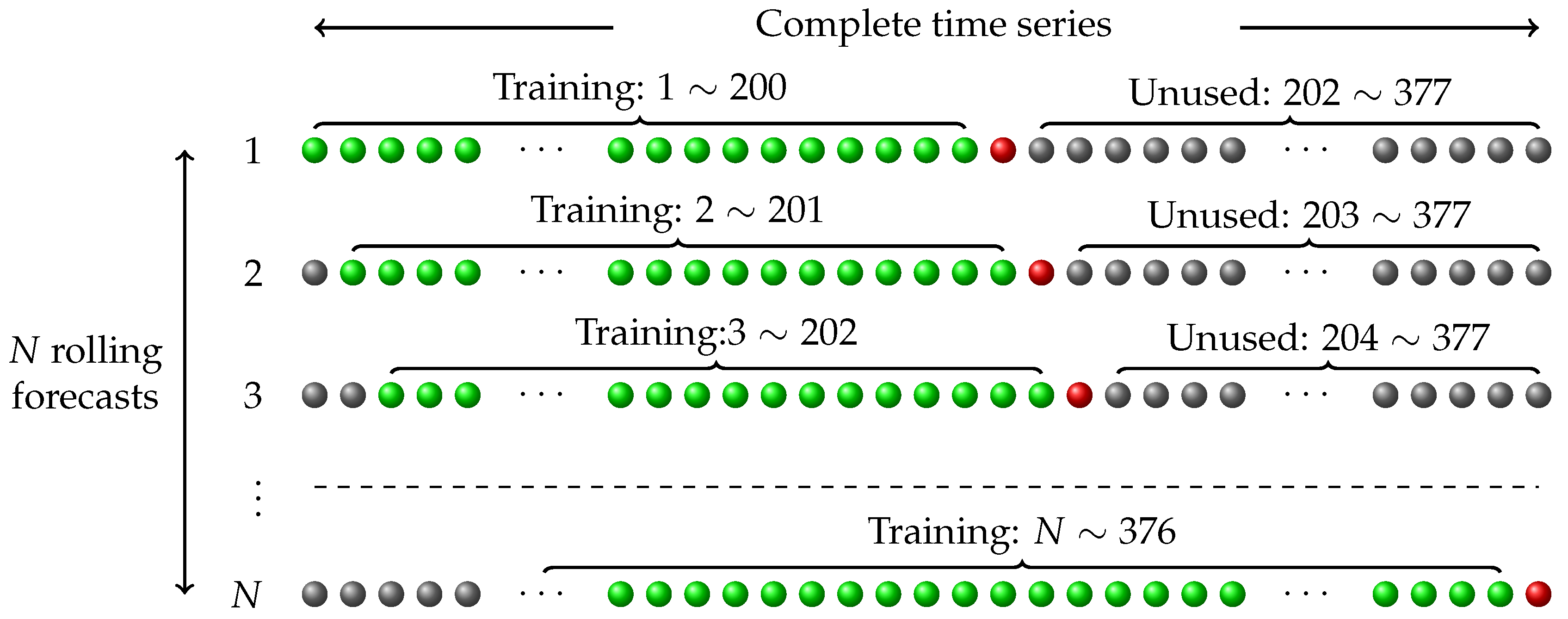
Rolling forecast is used in this paper. Data from the first 200 weeks are used to train the model, and thus generate the first forecast. A sliding window is then used to define the training data for subsequent forecasts. Given the span of the data (377 weeks), 177 pseudo out-of-sample forecasts can be made for each time series. This procedure is depicted in Figure 2. The mean absolute percentage errors (MAPEs) of UPC-level demand under each case are shown in the colored columns of Table 1.

The results shown in Table 1 agree very well with the hypothesized scenario, namely, the forecast errors of Cases I–IV follow a decreasing order. Models in Case I, namely, C1ets and C1arima, perform the worst because they can hardly capture any demand surge during the promotional periods. This strongly supports the conjecture that pricing and promotional strategy forms a relevant part of the suppliers’ information set, in the absence of which forecast errors may be significant. Case II performs better than Case I due to the additional information (past price and promotion) used during forecasting. However, the most interesting observation is that Case III performs almost as well as Case IV, with C3opt having a higher accuracy than C3bu.

The results shown in Table 1 can be used to conclude that, for the current dataset, sharing full information with a supplier no doubt benefits the supplier greatly. However, only sharing forecast information can also result in significant forecast improvements on the supplier’s side. The fact that forecast sharing benefits the supplier is not surprising; however, the observation that it nearly yields the same level of benefits as Case IV is quite interesting.

5.2. Forecast Accuracies of the Combined Forecasts

The second part of the empirical study investigates the effects of forecast combination on forecast accuracy. To simplify the case study, the full information set in Case IV is assumed to be available, so that all Cases I–III forecasts can be generated as well. In this way, a total of seven component models are used during forecast combination. Since all forecast combination methods, besides Avg and Trim, require training/fitting, 100 out of 177 sets of pseudo out-of-sample forecasts are randomly chosen for training. The remaining samples are used for error evaluation. The MAPEs of the combined UPC-level forecasts are shown in columns 9–15 of Table 1.

By contrasting the combined forecasts to the component forecasts, it is observed that the combined forecasts appear to be more accurate in general. For certain UPCs, such as “3828103123,” the worst combined forecasts are found to be better than the best component forecasts. Among the various forecast combination methods, Lad performs the best, whereas Avg performs the worst. Since the differences between the best and worst combined forecasts are smaller than that between the component forecasts, it seems that choosing combined forecasts is less risky than choosing the forecasts from the “best-known” component model. This also implies that, when the best forecasting method for a new UPC is unknown, it is better to choose a combined forecast than choosing a component forecast based on previous results. To elaborate, suppose only the forecasts for UPC “5300015132” are available, the forecaster would choose C1ets as the best-known model—based on its small MAPE of 15.13% for that UPC. In this case, C1ets would give large errors for other UPCs, which is not desired.

6. Conclusions

The benefits of forecast sharing in a supply chain in terms of forecast accuracy is demonstrated through an empirical example. Four cases characterized by different levels of information sharing are considered. It is found that the full information sharing case (Case IV) produces the best forecast accuracy. However, by only sharing the retailer-level forecast values (Case III), the forecast at the supplier level is almost as accurate as Case IV. This implies that it is not necessary for retailers to share pricing and promotional strategies explicitly, which protects them from leakage of sensitive competitive information. This concludes the first contribution of the paper.

When the retailer-level forecasts are shared, suppliers can reconcile those forecasts with their own forecasts. It is also shown that optimal reconciliation (which considers all forecasts) outperforms the traditional bottom-up method (which considers only the retailer-level forecasts). The merit of the optimal reconciliation approach is that it puts greater weights on the more accurate forecasts, so that the overall performance of all forecasts across the hierarchy can be improved. Additionally, forecast combination has been shown to improve the reliability of the forecasts, especially when the best component model is unknown to a forecaster. To that end, hierarchical reconciliation and forecast combination are two ways to address the forecast inconsistencies in supply-chain management, and hence conclude our second contribution.

References

- Niranjan, T.T.; Wagner, S.M.; Aggarwal, V. Measuring information distortion in real-world supply chains. Int. J. Prod. Res. 2011, 49, 3343–3362. [Google Scholar] [CrossRef]
- Ramanathan, U. Performance of supply chain collaboration—A simulation study. Expert Syst. Appl. 2014, 41, 210–220. [Google Scholar] [CrossRef]
- Wong, K.K.; Song, H.; Witt, S.F.; Wu, D.C. Tourism forecasting: To combine or not to combine? Tour. Manag. 2007, 28, 1068–1078. [Google Scholar] [CrossRef] [Green Version]
- Hibon, M.; Evgeniou, T. To combine or not to combine: selecting among forecasts and their combinations. Int. J. Forecast. 2005, 21, 15–24. [Google Scholar] [CrossRef]
- Palm, F.C.; Zellner, A. To combine or not to combine? Issues of combining forecasts. J. Forecast. 1992, 11, 687–701. [Google Scholar] [CrossRef]
- Bates, J.M.; Granger, C.W.J. The Combination of Forecasts. J. Oper. Res. Soc. 1969, 20, 451–468. [Google Scholar] [CrossRef]
- Gaur, V.; Giloni, A.; Seshadri, S. Information Sharing in a Supply Chain Under ARMA Demand. Manag. Sci. 2005, 51, 961–969. [Google Scholar] [CrossRef] [Green Version]
- Giloni, A.; Hurvich, C.; Seshadri, S. Forecasting and information sharing in supply chains under ARMA demand. IIE Trans. 2014, 46, 35–54. [Google Scholar] [CrossRef]
- Ali, M.M.; Boylan, J.E. Feasibility principles for Downstream Demand Inference in supply chains. J. Oper. Res. Soc. 2011, 62, 474–482. [Google Scholar] [CrossRef]
- Cui, R.; Allon, G.; Bassamboo, A.; Mieghem, J.A.V. Information Sharing in Supply Chains: An Empirical and Theoretical Valuation. Manag. Sci. 2015, 61, 2803–2824. [Google Scholar] [CrossRef] [Green Version]
- Ali, M.M.; Boylan, J.E. On the value of sharing demand information in supply chains. In Proceedings of the OR56 Annual Conference, London, UK, 9–11 September 2014; pp. 44–56. [Google Scholar]
- Gümüş, M. With or Without Forecast Sharing: Competition and Credibility under Information Asymmetry. Prod. Oper. Manag. 2014, 23, 1732–1747. [Google Scholar] [CrossRef]
- Özer, O.; Zheng, Y.; Ren, Y. Trust, Trustworthiness, and Information Sharing in Supply Chains Bridging China and the United States. Manag. Sci. 2014, 60, 2435–2460. [Google Scholar] [CrossRef] [Green Version]
- Özer, O.; Zheng, Y.; Chen, K.Y. Trust in Forecast Information Sharing. Manag. Sci. 2011, 57, 1111–1137. [Google Scholar] [CrossRef] [Green Version]
- Cachon, G.P.; Lariviere, M.A. Contracting to Assure Supply: How to Share Demand Forecasts in a Supply Chain. Manag. Sci. 2001, 47, 629–646. [Google Scholar] [CrossRef] [Green Version]
- Friedman, J.W. A Non-cooperative Equilibrium for Supergames. Rev. Econ. Stud. 1971, 38, 1–12. [Google Scholar] [CrossRef]
- Yagli, G.M.; Yang, D.; Srinivasan, D. Reconciling solar forecasts: Sequential reconciliation. Sol. Energy 2019, 179, 391–397. [Google Scholar] [CrossRef]
- Yang, D.; Quan, H.; Disfani, V.R.; Rodríguez-Gallegos, C.D. Reconciling solar forecasts: Temporal hierarchy. Sol. Energy 2017, 158, 332–346. [Google Scholar] [CrossRef]
- Yang, D.; Quan, H.; Disfani, V.R.; Liu, L. Reconciling solar forecasts: Geographical hierarchy. Sol. Energy 2017, 146, 276–286. [Google Scholar] [CrossRef]
- Hong, T.; Xie, J.; Black, J. Global energy forecasting competition 2017: Hierarchical probabilistic load forecasting. Int. J. Forecast. 2019. [Google Scholar] [CrossRef]
- Athanasopoulos, G.; Ahmed, R.A.; Hyndman, R.J. Hierarchical forecasts for Australian domestic tourism. Int. J. Forecast. 2009, 25, 146–166. [Google Scholar] [CrossRef] [Green Version]
- Yang, D.; Goh, G.S.W.; Jiang, S.; Zhang, A.N.; Akcan, O. Forecast UPC-level FMCG demand, Part II: Hierarchical reconciliation. In Proceedings of the IEEE International Conference on Big Data (Big Data), Santa Clara, CA, USA, 29 October–1 November 2015; pp. 2113–2121. [Google Scholar] [CrossRef]
- Bray, R.L.; Mendelson, H. Information Transmission and the Bullwhip Effect: An Empirical Investigation. Manag. Sci. 2012, 58, 860–875. [Google Scholar] [CrossRef] [Green Version]
- Chen, F.; Drezner, Z.; Ryan, J.K.; Simchi-Levi, D. Quantifying the Bullwhip Effect in a Simple Supply Chain: The Impact of Forecasting, Lead Times, and Information. Manag. Sci. 2000, 46, 436–443. [Google Scholar] [CrossRef] [Green Version]
- Hyndman, R.J.; Ahmed, R.A.; Athanasopoulos, G.; Shang, H.L. Optimal combination forecasts for hierarchical time series. Comput. Stat. Data Anal. 2011, 55, 2579–2589. [Google Scholar] [CrossRef] [Green Version]
- Hyndman, R.J.; Lee, A.J.; Wang, E. Fast computation of reconciled forecasts for hierarchical and grouped time series. Comput. Stat. Data Anal. 2016, 97, 16–32. [Google Scholar] [CrossRef] [Green Version]
- Wickramasuriya, S.L.; Athanasopoulos, G.; Hyndman, R.J. Forecasting Hierarchical and Grouped Time Series through Trace Minimization; Working Paper 15/15; Department of Econometrics & Business Statistics, Monash University: Melbourne, Australia, 2015. [Google Scholar]
- Granger, C.W.J. Invited review combining forecasts—Twenty years later. J. Forecast. 1989, 8, 167–173. [Google Scholar] [CrossRef]
- Yang, D.; Dong, Z. Operational photovoltaics power forecasting using seasonal time series ensemble. Sol. Energy 2018, 166, 529–541. [Google Scholar] [CrossRef]
- Wang, Y.; Zhang, N.; Tan, Y.; Hong, T.; Kirschen, D.S.; Kang, C. Combining Probabilistic Load Forecasts. IEEE Trans. Smart Grid 2019, 10, 3664–3674. [Google Scholar] [CrossRef]
- Baran, S.; Lerch, S. Combining predictive distributions for the statistical post-processing of ensemble forecasts. Int. J. Forecast. 2018, 34, 477–496. [Google Scholar] [CrossRef] [Green Version]
- De Menezes, L.M.; Bunn, D.W.; Taylor, J.W. Review of guidelines for the use of combined forecasts. Eur. J. Oper. Res. 2000, 120, 190–204. [Google Scholar] [CrossRef]
- Berry, S.; Levinsohn, J.; Pakes, A. Automobile Prices in Market Equilibrium. Econometrica 1995, 63, 841–890. [Google Scholar] [CrossRef]
- Nevo, A. Measuring Market Power in the Ready-to-Eat Cereal Industry. Econometrica 2001, 69, 307–342. [Google Scholar] [CrossRef] [Green Version]
- Muller-Navarra, M.; Lessmann, S.; Voss, S. Sales Forecasting with Partial Recurrent Neural Networks: Empirical Insights and Benchmarking Results. In Proceedings of the 48th Hawaii International Conference on System Sciences (HICSS), Kauai, HI, USA, 5–8 January 2015; pp. 1108–1116. [Google Scholar] [CrossRef]
- Fildes, R.; Nikolopoulos, K.; Crone, S.F.; Syntetos, A.A. Forecasting and operational research: A review. J. Oper. Res. Soc. 2008, 59, 1150–1172. [Google Scholar] [CrossRef]
- Fildes, R.; Goodwin, P.; Lawrence, M.; Nikolopoulos, K. Effective forecasting and judgmental adjustments: an empirical evaluation and strategies for improvement in supply-chain planning. Int. J. Forecast. 2009, 25, 3–23. [Google Scholar] [CrossRef]
- Ali, O.G.; Sayin, S.; van Woensel, T.; Fransoo, J. SKU demand forecasting in the presence of promotions. Expert Syst. Appl. 2009, 36, 12340–12348. [Google Scholar] [CrossRef]
- Huang, T.; Fildes, R.; Soopramanien, D. The value of competitive information in forecasting FMCG retail product sales and the variable selection problem. Eur. J. Oper. Res. 2014, 237, 738–748. [Google Scholar] [CrossRef]
- Tibshirani, R. Regression Shrinkage and Selection via the Lasso. J. R. Stat. Soc. Ser. B (Methodol.) 1996, 58, 267–288. [Google Scholar] [CrossRef]
- Toro-González, D.; McCluskey, J.J.; Mittelhammer, R.C. Beer Snobs do Exist: Estimation of Beer Demand by Type. J. Agric. Resour. Econ. 2014, 39, 174–187. [Google Scholar]
- Jami, A.; Mishra, H. Downsizing and Supersizing: How Changes in Product Attributes Influence Consumer Preferences. J. Behav. Decis. Mak. 2014, 27, 301–315. [Google Scholar] [CrossRef]
- Chahrour, R.A. Sales and price spikes in retail scanner data. Econ. Lett. 2011, 110, 143–146. [Google Scholar] [CrossRef]
Figure 1.
A three-level hierarchical demand time series structure. Universal product code (UPC) level, , contains n nodes; retailer level, , contains nodes.
Figure 2.
Experimental design, following Yang et al. [22]. A total of rolling forecasts are performed for each UPC time series. The data point being forecast is shown in red. The size of training window (shown in green) is fixed at 200.