Adaptive Inverse Controller Design Based on the Fuzzy C-Regression Model (FCRM) and Back Propagation (BP) Algorithm

Abstract

Establishing an accurate inverse model is a key problem in the design of adaptive inverse controllers. Most real objects have nonlinear characteristics, so mathematical expression of an inverse model cannot be obtained in most situation. A Takagi–Sugeno(T-S)fuzzy model can approximate real objects with high precision, and is often applied in the modeling of nonlinear systems. Since the consequent parameters of T-S fuzzy models are linear expressions, this paper firstly uses a fuzzy c-regression model (FCRM) clustering algorithm to establish inverse fuzzy model. As the least mean square (LMS) algorithm is only used to adjust consequent parameters of the T-S fuzzy model in the process of parameter adjustment, the premise parameters are fixed and unchanged in the process of adjustment. In this paper, the back propagation (BP) algorithm is applied to adjust the premise and consequent parameters of the T-S fuzzy model, simultaneously online. The simulation results show that the error between the system output controlled by proposed adaptive inverse controller and the desired output is smaller, also the system stability can be maintained when the system output has disturbances.

1. Introduction

The inverse problem has been a research hotspot in recent years; the basic idea of the inverse problem is to use the results and some general principles (or models) to determine the parameters (or model parameters) that represent the characteristics of the problem. In general, the estimation parameters were decided by operation or experimental data. The inverse problem was usually implemented by artificial intelligence algorithms, which had the function of learning and reasoning, such as the simulated annealing algorithm, tabu search algorithm, fuzzy clustering algorithm, improved NSGA-III algorithm [1], krill herd algorithm [2,3,4], and so on. For example, Nino-Ruiz proposed two efficient and practical implementations of local search methods based on tabu search and simulated annealing to solve inverse problem [5]. In article [6], improved tabu search and simulated annealing methods were utilized for nonlinear data assimilation using local search methods, which is an inverse problem.

In many real control problems, the mathematical model of the controlled object or process was difficult to determine prior. As there is a lack of exact mathematical model of the controlled object, data driving modeling methods were used for modeling of the controlled object, such as artificial neural network systems, fuzzy systems, and so on. These methods included the mathematical optimization process, which determined model parameters by system operation input and output data, called training data. The training data should cover the whole operation condition as much as possible. Even if the system model was obtained under certain conditions, its dynamic parameters and structure may change when the working conditions change. In this situation, adaptive control was proposed to compensate for unpredictable changes in model order, parameters, and input signals. Adaptive control was a model based controller, which is needed to improve the model during the operation of the system. This process includes online parameter adjustment, and through online adjustment, the model will become more and more accurate and closer to the real process.

The following problems still existed in the research of adaptive control theory: stability, convergence, and how to select a proper performance index. Sen presented a robust adaptive stabilization scheme for a class of nominally first-order hybrid systems [7] and had wider stability conditions, however, a stabilization scheme for high order hybrid systems was not discussed. In [8], a robustly stable multiestimation scheme was proposed for an adaptive controller and it estimated reduced-order plant models for the original controller plant. In article [9], adaptive control was applied for a non-linearly parameterized pure-feedback system, where a parameter separation technique had been designed to derive the adaptive laws.

Adaptive inverse control was first proposed by Widrow in 1986 and then caught the interest of other researchers [10]. The basic idea of adaptive inverse control was to drive the controller object with a signal, and the control signal was the inverse of the controller object itself. The adaptive filtering method was adapted to identify the inverse model of controlled object. The feedback in adaptive inverse control belonged to local feedback, which was only used to change model parameters in the process of adaptive iteration. It did not directly control the signal flow in the main loop, nor the closed-loop output to the input, so it was an open-loop control. Compared with a general adaptive controller, the inverse model of a controlled object was connected with the controlled object, so inverse model output acted as the input of the controlled object, and the adaptive inverse controller parameters were adjusted online, thus the output of the controlled object can track the desired set value. So the main issue is how to get the inverse model of the controlled object. The necessary condition for the existence of adaptive inverse controller is that the controlled object is reversible and the mapping of output to input is single-valued. In the actual industrial process, in most cases, it is impossible to get the exact mathematical expression of the object’s inverse model. In the design of adaptive inverse controllers, intelligent identification methods are usually utilized to get the inverse model of the controlled object, such as in volterra basis function networks [11,12], neural networks [13,14], fuzzy systems [15,16] and so on. Among them, the adaptive inverse fuzzy controller based on the fuzzy model was widely used. Commonly included are the T-S fuzzy model based on the fuzzy tree model [17], T-S fuzzy model based on the grid method [18], T-S fuzzy model based on entropy clustering and fuzzy partition [19], recursive least squares support vector machine [20], type 2 fuzzy model [21,22,23], and so on. In practice, adaptive inverse control has also been successfully applied, including in pneumatic loading systems [24], cable-driven parallel systems [25,26], pH neutralization processes [27], and chatter vibrations in internal turning operations [28].

Although the inverse model can control the object accurately in theory, the actual operating conditions of the object are complex and changeable, and the inverse model based on the input and output data of a certain period of time cannot cover the whole operating conditions of the controlled object. Therefore, in the actual adaptive inverse control process, the inverse model parameters need to be adjusted online. Due to its simple implementation and fast convergence, the least mean square (LMS) algorithm was widely used in online parameter adjustment of adaptive inverse controller [29]. The big bang-big crunch optimization algorithm was also applied in the turning of inverse model parameters [30].

The T-S fuzzy model was widely used in the design of adaptive inverse fuzzy controller. Its consequent form is a linear expression and it has high identification accuracy. The distance of the fuzzy c-regression model (FCRM) clustering algorithm was described by point to surface, which was consistent with the form of consequent parameters of T-S fuzzy model. In this article, the FCRM clustering algorithm is used to establish the T-S fuzzy inverse model, which is an estimating of parameters for the T-S fuzzy inverse model. Compared with article [5,6], where the FCRM clustering algorithm is applied to determine model parameters and tabu search and simulated annealing methods were adopted. The adaptive inverse controller based on the least mean square (LMS) algorithm only adjusts consequent parameters of T-S fuzzy model, and premise parameters are fixed. In this article, the back propagation (BP) algorithm is used to adjust the parameters of the T-S fuzzy model online in the parameter adjustment stage of fuzzy inverse model. Compared with LMS, the proposed algorithm has more number of parameters adjusted online. The simulation results show that the proposed adaptive inverse controller has smaller errors and when system output has disturbances, the controller has stronger robustness.

2. T-S Fuzzy Model

The T-S fuzzy model can be described by the following if-then fuzzy rules [31]:

$$\begin{gathered} R^i:if x_1 is A_1^i and \cdots and x_M is A_M^i \mathrm{then} y_i=p_1^i{x}_1+\cdots +p_M^i{x}_M+p_0^i \\ \mathrm{and} y=\frac{{\displaystyle \sum _{i=1}^c{\mu }^i{y}_i}}{{\displaystyle \sum _{i=1}^c{\mu }^i}}, {\mu }^i={\displaystyle \prod _{j=1}^M{A}_j^i(x_j)} \end{gathered}$$

where i = 1,2,…,c, c is the number of fuzzy rules, x_j (j = 1,2,…,M) is the system input, y_i is the i-th rule output, $A_j^i$ (j = 1,2,…,M) is the fuzzy sets of input spatial and $p_j^i$ (j = 1,2,…,M) is the consequent parameter of the i-th rule.

If all input variables are considered as an input vector, then the alternative T-S fuzzy model can be described as [32]:

$$R^i: \mathit{if}\mathit{x} \mathrm{is} {\mathit{A}}^{\mathit{i}}\mathrm{then} y_i=p_1^i{x}_1+\cdots +p_M^i{x}_M+p_0^i$$

where x = [x₁,x₂,…,x_M] is the input variables vector. The fuzzy clustering algorithm was widely used for this alternative T-S fuzzy model identification, then Aⁱ will be the fuzzy membership degree x belong to the i-th class (i-th rule). Thus the premise parameter can be calculated easily.

3. T-S Fuzzy Model Identification Using FCRM

Suppose there are N (N > 1) sets of input–output data {(x_k, y_k)}(k = 1,2,…,N) to be clustered, input vector x_k can be expressed as [x_1k,…,x_Mk]^T and y_k denotes the output. The fuzzy c-regression model clustering algorithm is carried out on these clustering data, and the data with same functional relation will group together. The functional cluster representative of FCRM is described as follow [33]:

$$y_i=p_1^i{x}_1+\dots +p_M^i{x}_M+p_0^i=[{\mathit{x}}^T,1]{\mathit{\theta }}_i$$

(1)

where i = 1,2,…,c, 2 ≤ c < N, ${\mathit{\theta }}_i={[p_1^i,\dots ,p_M^i,p_0^i]}^T$. If FCRM clustering generates c clusters, then there will be c fuzzy rules corresponding to the T-S fuzzy model. Compared with the fuzzy c-means (FCM) clustering algorithm, the sample distance of FCRM is denoted as follows:

$$d_{ik}=\left|{\widehat{\mathit{x}}}_k{\mathit{\theta }}_i-y_k\right|$$

(2)

where ${\widehat{\mathit{x}}}_k=[{\mathit{x}}_k^T,1]$, k = 1,2,…,N, i = 1,2,…,c. Set a c × N matrix U = [u_ik] to represent the degree of input–output data (x_k,y_k) belonging to the i-th class. According to the fuzzy clustering algorithm, U should satisfy the following constrains:

$${\displaystyle \sum _{i=1}^c{u}_{ik}=1,0<{\displaystyle \sum _{k=1}^N{u}_{ik}<N}}.$$

(3)

The aim of FCRM is to minimize the objective function:

$$J_m(\mathit{U},{\mathit{\theta }}_1,\dots ,{\mathit{\theta }}_c)={\displaystyle \sum _{k=1}^N{\displaystyle \sum _{i=1}^c{(u_{ik})}^m{(d_{ik})}^2}}$$

(4)

The Lagrange multiplier method was adopted to solve this problem. First we constructed the Lagrange function as follows:

$$F(\lambda ,u_{ik})={\displaystyle \sum _{i=1}^c{(u_{ik})}^m{(d_{ik}({\mathit{\theta }}_i))}^2-\lambda ({\displaystyle \sum _{i=1}^c{u}_{ik}-1})}.$$

(5)

Then we calculated the partial derivative of F to u_ik and λ and made the partial derivative equal to 0:

$$\frac{\partial F(\lambda ,u_{1k},\cdots ,u_{ck})}{\partial u_{ik}}=m{(u_{ik})}^{m-1}{(d_{ik}({\mathit{\theta }}_i))}^2-\lambda =0$$

(6)

$$\frac{\partial F(\lambda ,u_{1k},\cdots u_{ck})}{\partial \lambda }=-({\displaystyle \sum _{i=1}^c{u}_{ik}-1)=0}$$

(7)

Due to d_ik(θ_i) > 0 by Equation (2), from Equations (6) and (7), u_ik can be calculated as follows:

$$u_{ik}=\frac{{(1/d_{ik}({\mathit{\theta }}_i))}^{\frac{2}{m-1}}}{{\displaystyle \sum _{l=1}^c{(1/d_{lk}({\mathit{\theta }}_l))}^{\frac{2}{m-1}}}}.$$

(8)

In Equation (8), 1 ≤ i ≤ c, 1 ≤ k ≤ N, θ_i can be calculated by weighted recursive least squares as follows:

$${\mathit{\theta }}_i={[{\mathit{X}}_a^T{\mathit{W}}_i{\mathit{X}}_a]}^{-1}{\mathit{X}}_a^T{\mathit{W}}_i\mathit{Y}$$

(9)

where:

$${\mathit{X}}_{\alpha }=\left[\begin{array}{l}{\mathit{x}}_1^T,1\\ {\mathit{x}}_2^T,1\\ ⋮\\ {\mathit{x}}_N^T,1\end{array}\right]\in {\mathit{R}}^{N\times (M+1)},\mathit{Y}=\left[\begin{array}{l}{y}_1\\ y_2\\ ⋮\\ y_N\end{array}\right]\in {\mathit{R}}^N,{\mathit{W}}_i=\left[\begin{array}{cccc}{u}_{i1}& 0& \cdots & 0\\ 0& u_{i2}& \cdots & 0\\ ⋮& ⋮& \ddots & ⋮\\ 0& 0& \cdots & u_{iN}\end{array}\right]\in {\mathit{R}}^{N\times N}$$

(10)

The right-hand-side matrix inverse of Equation (9) may not exist. In order to avoid matrix inverse calculation, an analytical solution was utilized as follows [34]:

$${\theta }_{ij}=\frac{{\displaystyle \sum _{k=1}^N{(u_{ik})}^m(y_k-{\displaystyle \sum _{t\ne j}{\theta }_{it}{\widehat{x}}_{kt}){\widehat{x}}_{kj}}}}{{\displaystyle \sum _{k=1}^N{(u_{ik})}^m{\widehat{x}}_{kj}^2}}.$$

(11)

Here i = 1,...,c and j (or t) = 1,…,M + 1.

The premise parameter is decided by the Gaussian membership function as follows:

$${\mu }_j^i(x_{jk})=\exp (-{(\frac{x_{jk}-{\alpha }_j^i}{{\beta }_j^i})}^2)$$

(12)

$${\alpha }_j^i=\frac{{\displaystyle \sum _{k=1}^N{u}_{ik}{x}_{jk}}}{{\displaystyle \sum _{k=1}^N{u}_{ik}}},{\beta }_j^i=\sqrt{\frac{2{\displaystyle \sum _{k=1}^N{u}_{ik}{(x_{jk}-{\alpha }_j^i)}^2}}{{\displaystyle \sum _{k=1}^N{u}_{ik}}}}$$

(13)

where i = 1,2,…,c, j = 1,2,…,M, k = 1,2,…,N.

4. Proposed Algorithm

4.1. Inverse Modeling Using FCRM

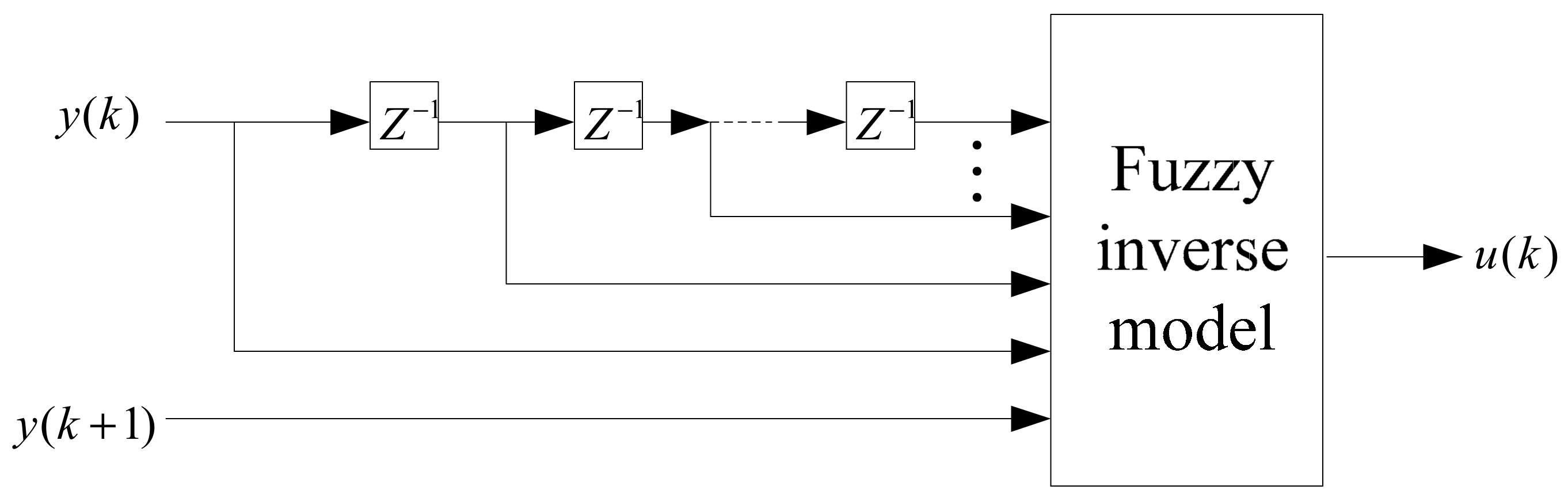
In order to establish the fuzzy inverse model of the controlled object, N sets of input–output pairs of the object are obtained using the experimental method. In this paper, a simple input simple output (SISO) system is considered. The output of the inverse model is the input of the current time of the positive model, and the inputs are the lagging link of the output and current time output of the positive model, as shown in Figure 1 [16]. Here z⁻¹ in Figure 1 stands for one-step delay.

In this paper, FCRM clustering algorithm is used for fuzzy inverse identification and the procedure is as follows:

• Step 1. Initialize matrix U⁰(c×N) to satisfy the Constrains (3), the clustering number c, parameter m (usually m = 2), termination threshold ε > 0, and maximum number of iterations Cyc, set r = 1;
• Step 2. Calculate the r-th iteration ${\mathit{\theta }}_i^r$ by Equation (11);
• Step 3. Calculate the r-th iteration $u_{ik}^r$ by Equation (8), if matrix norms ||U^r− U^r-1|| < ε, or the iteration variation r equal to Cyc, go to Step 4, else r = r + 1 and go to Step 2;
• Step 4. Calculate the premise parameter by Equation (13);
• Step 5. The consequent parameters of T-S fuzzy model are the θ values obtained by FCRM clustering algorithm.

4.2. Online Adaptive Inverse Controller Structure

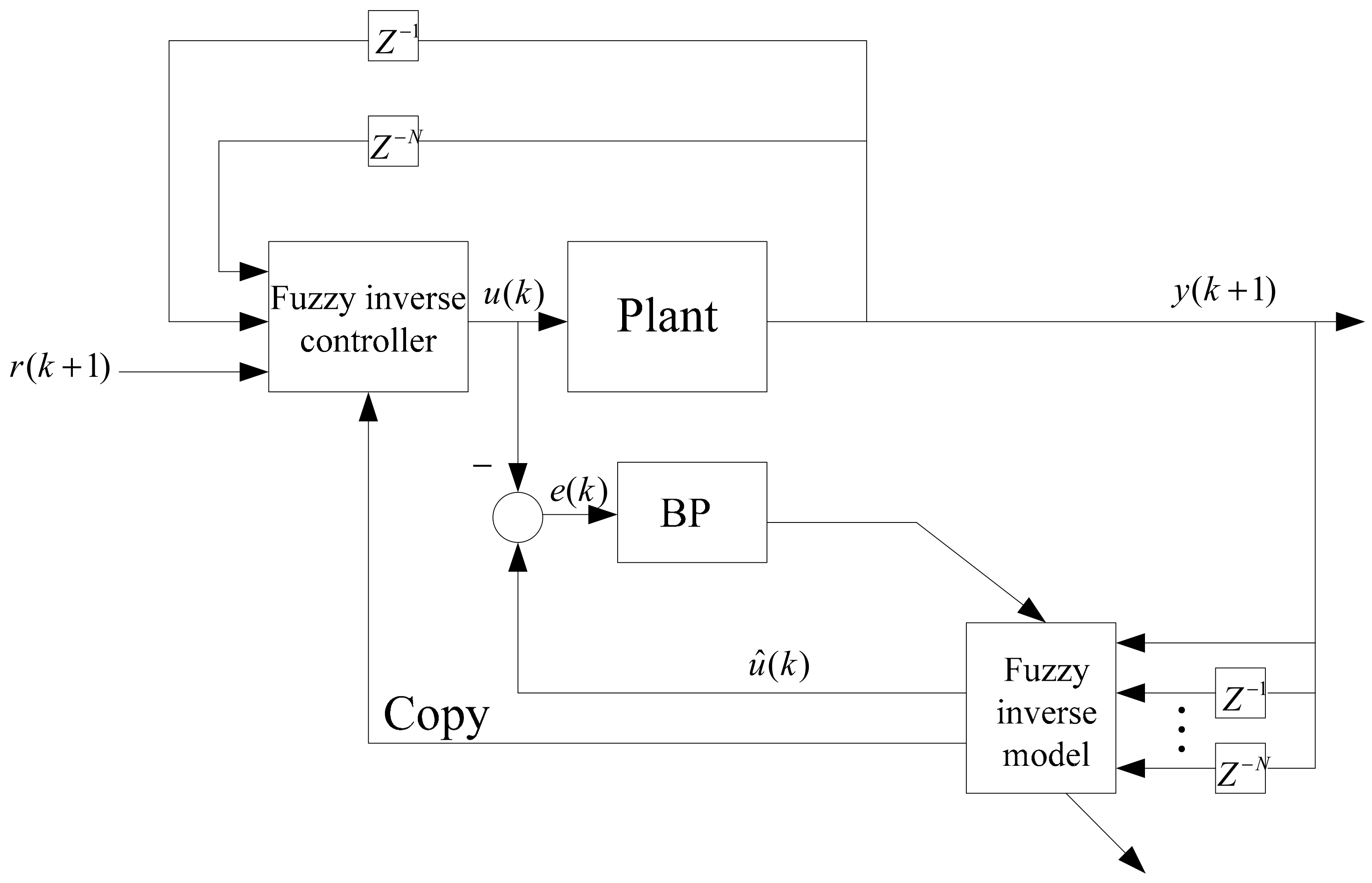
In this paper, the adaptive fuzzy control is connected in series with the controlled plant, and the output of the inverse model is taken as the input of the controlled plant. The output of the controlled plant is fed back to the input of the inverse model to get the output of the inverse model. The output of fuzzy inverse model is compared with the output of the inverse controller, which produces deviation. The premise and consequent parameters of the fuzzy inverse model are adjusted by the BP algorithm, which can be shown as in Figure 2.

The adjusted fuzzy inverse model replaces the original fuzzy inverse controller in the next sampling period, so the output of the controlled plant can track the reference input with high precision.

4.3. Online Parameter Adjustment

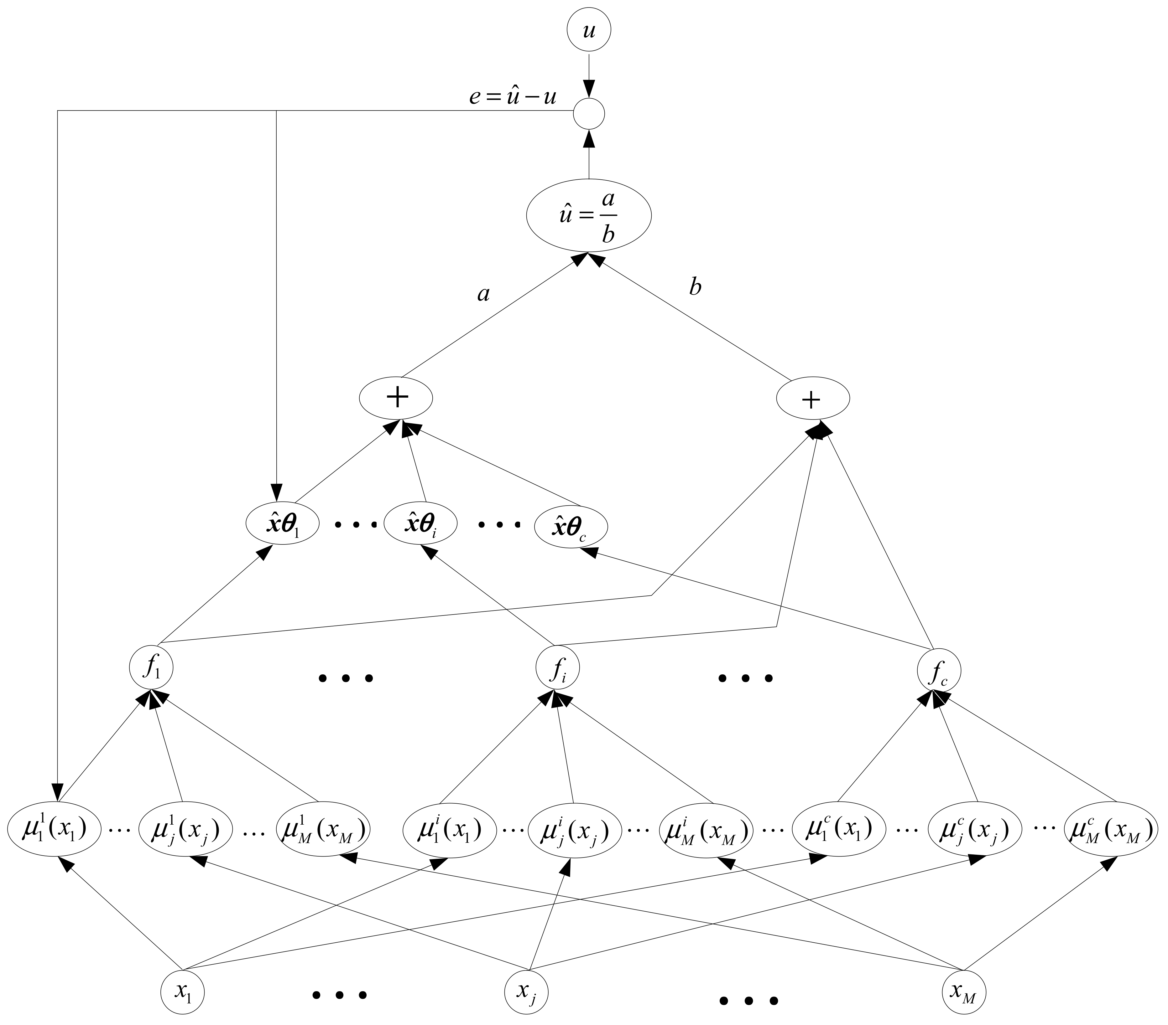
BP algorithm (error back propagation algorithm) is a learning algorithm suitable for a multilayer neural network. It is based on a gradient descent method, that is, Newton’s method, and consists of a forward propagation process and back propagation. In the process of forward propagation, the input information is processed layer by layer through the input layer and hidden layer and then transmitted to the output layer. If the desired output value is not obtained at the output layer, then the sum of the square of error between system output and desired output is taken as the objective function and transferred to back propagation. Then the partial derivative of the objective function to the weight of each neuron is calculated layer by layer, as the basis for modifying the weight, so the learning of the network is completed in the process of weight modification. When the error reaches the expected value, the network learning ends. The BP algorithm diagram can be seen from Figure 3.

In Figure 3,

$$\begin{gathered} \widehat{\mathit{x}}=[x_1,x_2,\cdots ,x_M,1] \\ {\mu }_j^i(x_j)=\exp (-{(\frac{x_j-{\alpha }_j^i}{{\beta }_j^i})}^2) \\ {f}_i={\displaystyle \prod _{j=1}^M{\mu }_j^i}(x_j) \\ a={\displaystyle \sum _{i=1}^c{f}_i\widehat{\mathit{x}}{\mathit{\theta }}_i} \\ b={\displaystyle \sum _{i=1}^c{f}_i}. \end{gathered}$$

As described in Section 3, the premise parameters of the T-S fuzzy model established by the FCRM clustering algorithm are described by the Gaussian membership function, so the adjustment parameters implemented by the BP algorithm include three characteristic parameters, including the center ${\alpha }_j^i$, and width ${\beta }_j^i$ (i = 1,2,…,c, j = 1,2,…,M) in the Gaussian membership function and consequent parameter θ of the T-S fuzzy model.

The updating process of the parameters can be described as follows:

(1)

$e(k)=\widehat{u}(k)-u(k)$

(2)

Updating ${\alpha }_j^i$:

$${\alpha }_j^i(k+1)={\alpha }_j^i(k)-{\eta }_{\alpha }\frac{\partial e}{\partial {\alpha }_j^i}$$

(14)

where $\frac{\partial e}{\partial {\alpha }_j^i}=2e(k){\overline{\omega }}_i(y_i-\widehat{u}(k))\frac{x_j-{\alpha }_j^i}{{({\beta }_j^i)}^2}$ and y_i is shown as Equation (1).

(3)

Updating ${\beta }_j^i$:

$${\beta }_j^i(k+1)={\beta }_j^i(k)-{\eta }_{\beta }\frac{\partial e}{\partial {\beta }_j^i}$$

(15)

where $\frac{\partial e}{\partial {\beta }_j^i}=2e(k){\overline{\omega }}_i(y_i-\widehat{u}(k))\frac{{(x_j-{\alpha }_j^i)}^2}{{({\beta }_j^i)}^3}$.

(4)

Updating θ:

$${\mathit{\theta }}_i(k+1)={\mathit{\theta }}_i(k)-{\eta }_{\theta }\frac{\partial e}{\partial {\mathit{\theta }}_i}$$

(16)

where $\frac{\partial e}{\partial {\mathit{\theta }}_i}=2e(k){\mathit{\psi }}_i$ and ${\mathit{\psi }}_i=[{\overline{\omega }}_i{x}_1\cdots {\overline{\omega }}_i{x}_M {\overline{\omega }}_i]$.

From Section 2, ${\overline{\omega }}_i$ in Equations (14)–(16) is described as:

$${\overline{\omega }}_i={\mu }_i/{\displaystyle \sum _{i=1}^c{\mu }_i}$$

(17)

η_α, η_β and η_θ are the learning rates of ${\alpha }_j^i$,${\beta }_j^i$, and θ, and admissibility values of η_α,η_β and η_θ are ranging from 0 to 2. If these values are too small, system convergence speed will be slow, and on the contrary, if these values are too large, the system will divergent.

5. Simulation Examples

5.1. Simulation 1

The following discrete object is selected for this example:

$$y(k+1)=\frac{y(k)u(k)}{1+y^2(k)}-\tan (u(k)).$$

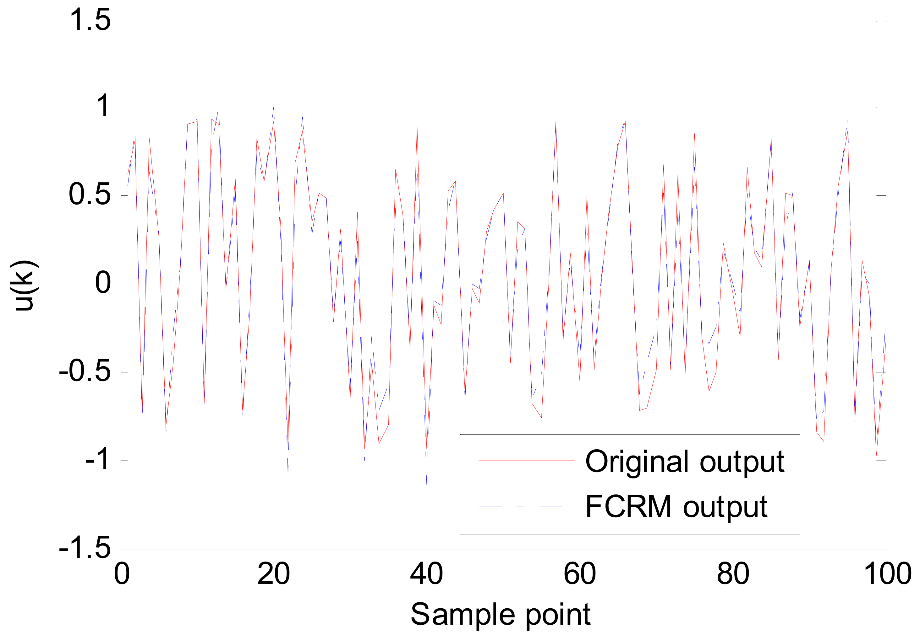
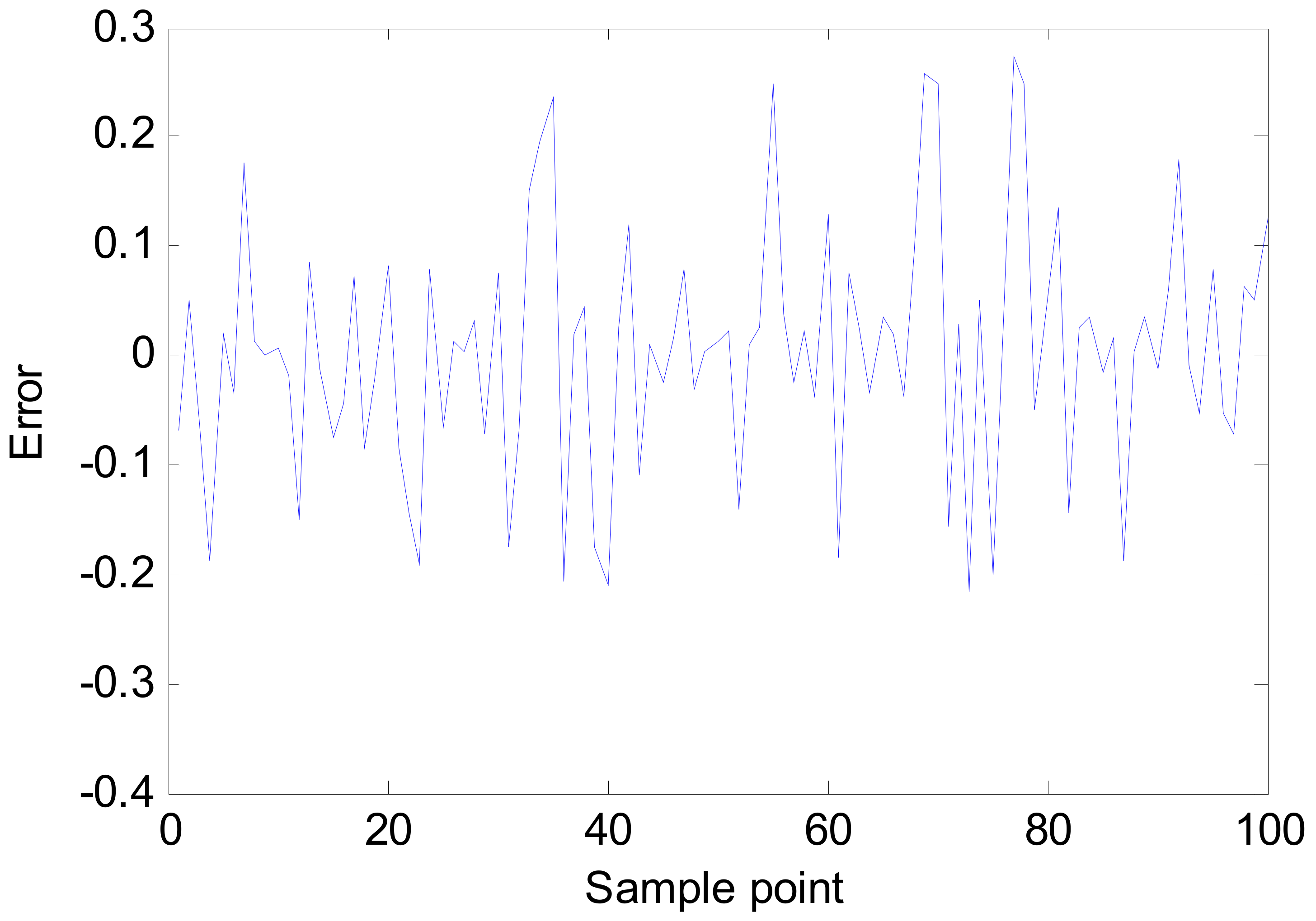
The positive model of the object is y(k + 1) = f(y(k),u(k)), so the inverse model is u(k) = g(y(k),y(k + 1)). In this paper, the inverse model of the object is established by the FCRM clustering algorithm. Firstly, the random number with uniform distribution is produced as the input u(k) of the system in the interval [−1, 1]. Through the object model, 100 pairs of input and output pairs are generated to establish the inverse model. The number of clustering (number of fuzzy rules) chosen in this case is 4, and in simulation 1, η_α = η_β = η_θ = 1.4. Figure 4 shows the output curve of FCRM clustering logarithm inverse model and sample, and Figure 5 shows the errors.

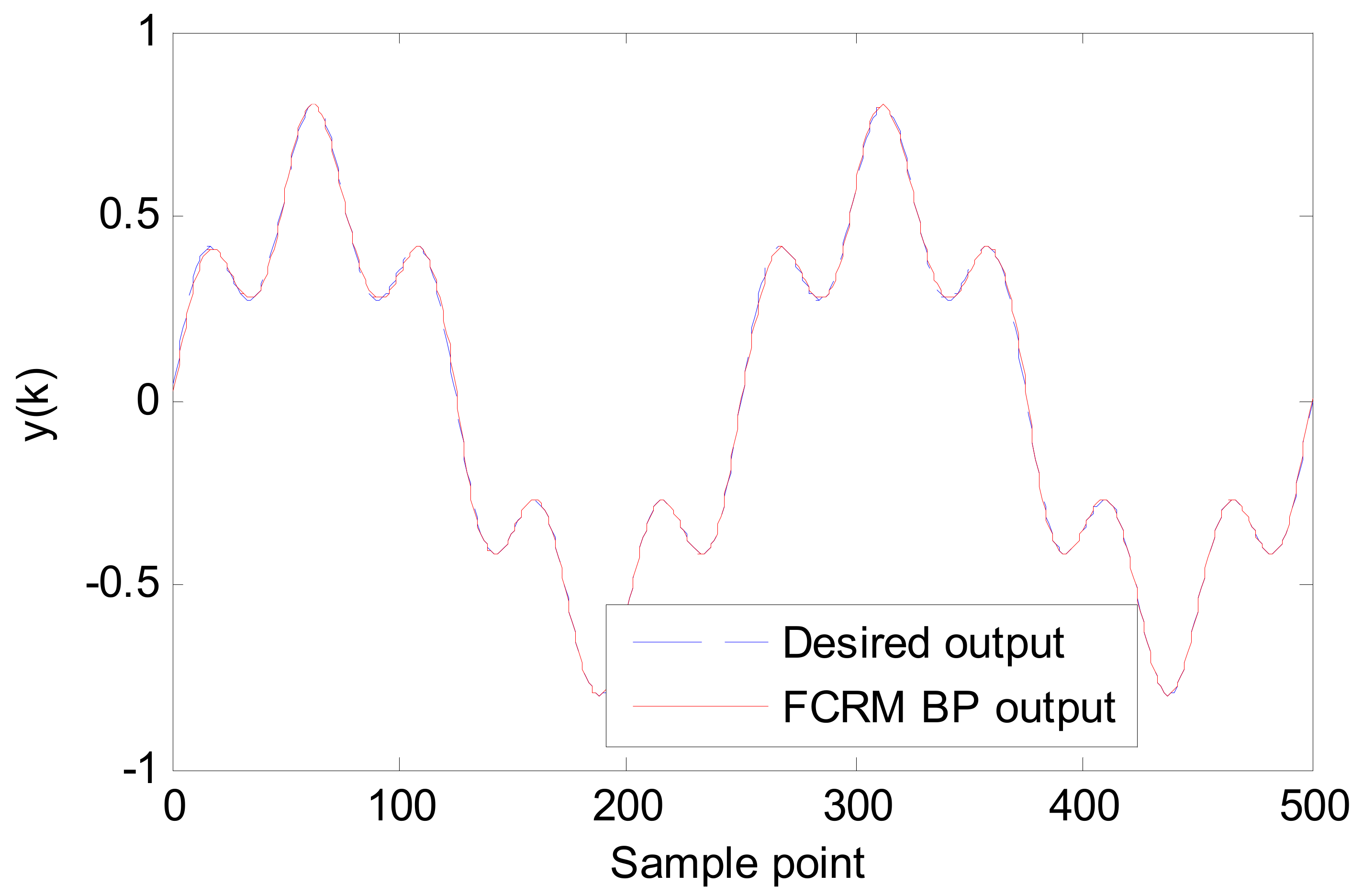
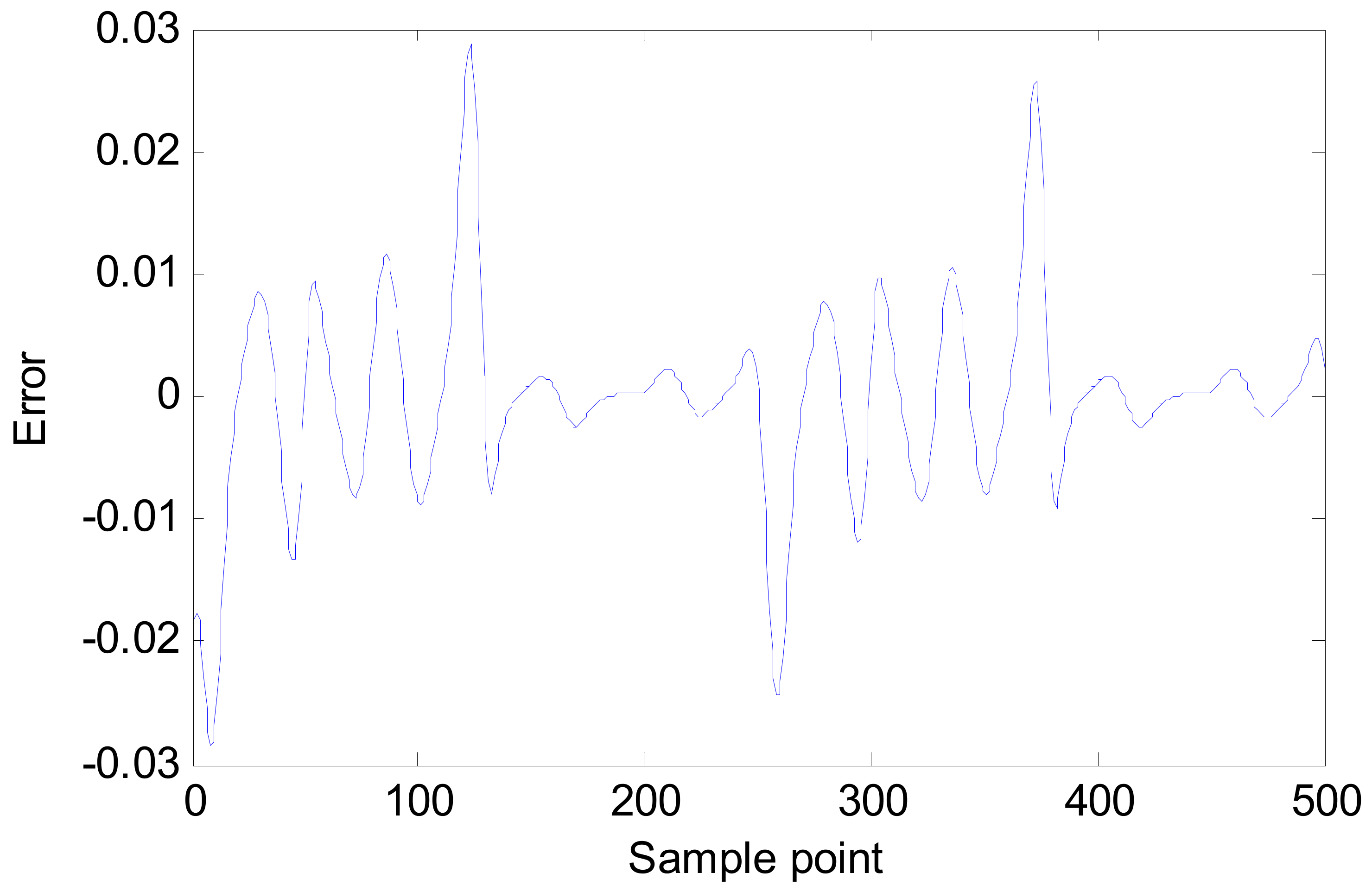
In this simulation, the desired output of the system is set to be r(k) = 0.6 sin(2kπ/250) + 0.2 sin (2kπ/250). Figure 6 shows the output curve of proposed method and desired output and Figure 7 shows the errors.

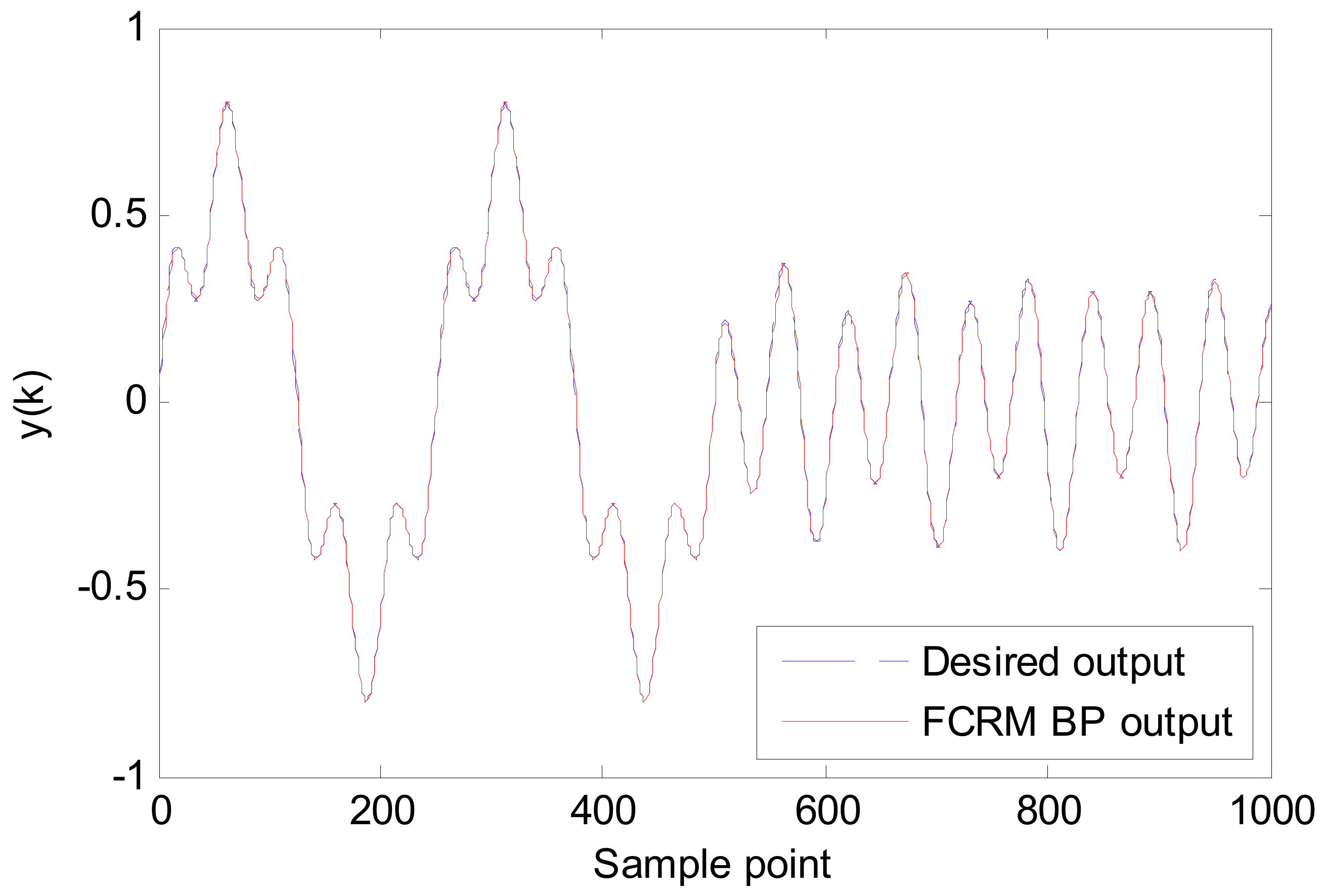
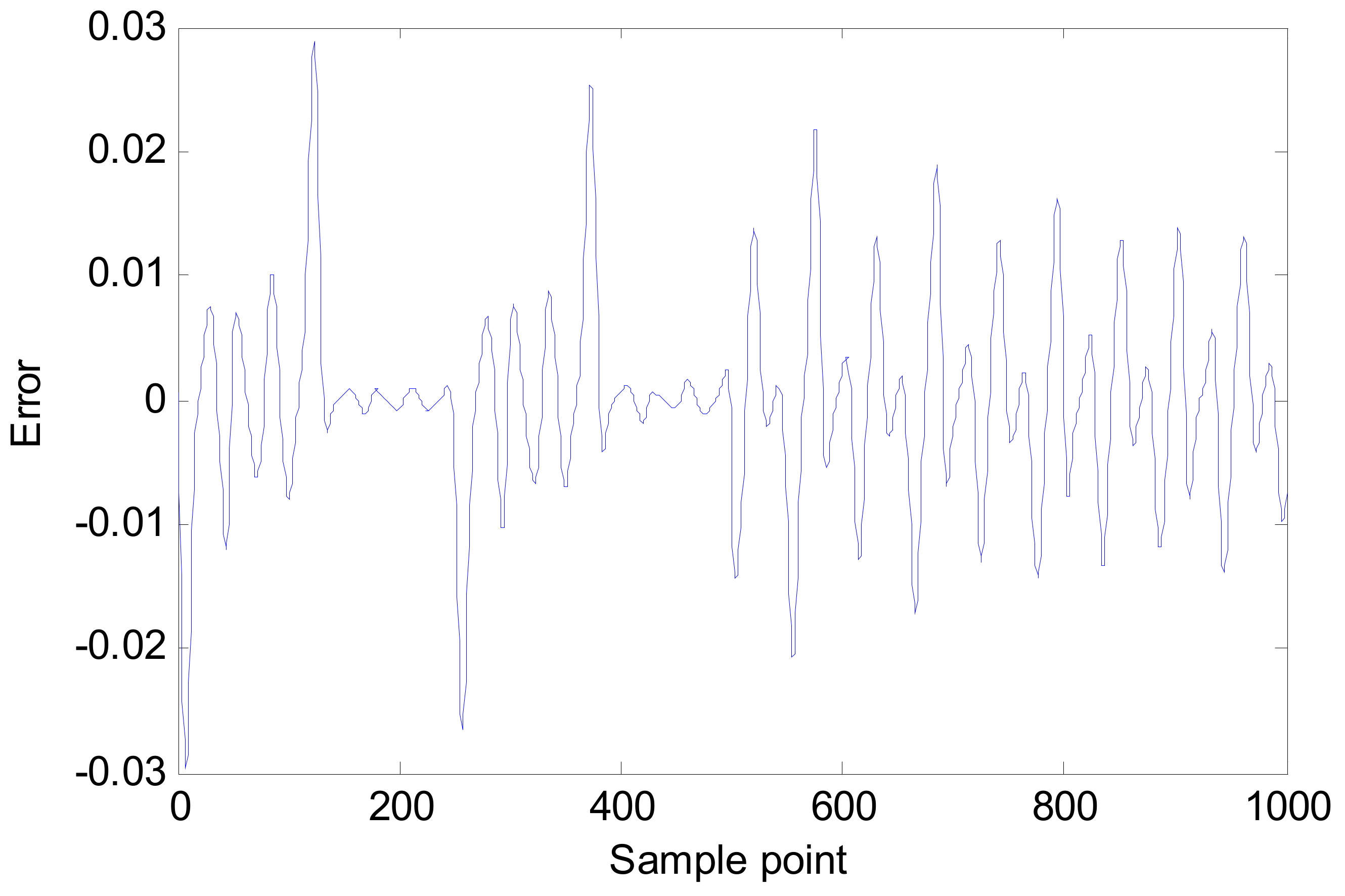
In order to further illustrate the control effect of this algorithm, at step 500, the desired output is set to be r(k) = 0.3 sin (2kπ/55) + 0.1 sin (2kπ/105). Figure 8 shows the output curve of the proposed method and the desired output, and Figure 9 shows the errors.

Table 1. Comparison of tracking accuracy for several adaptive interval controller.

Inverse Controller	No. of Rules	RMSE
Fuzzy tree [7]	4	0.0286
Fuzzy partition-LMS [6]	4	0.0261
Type 2 fuzzy model [8]	4	0.0132
FCM-LMS	4	0.0158
FCRM-BP	4	0.0074

compared our method and other inverse controllers tracking accuracy under simulation 1000 steps.

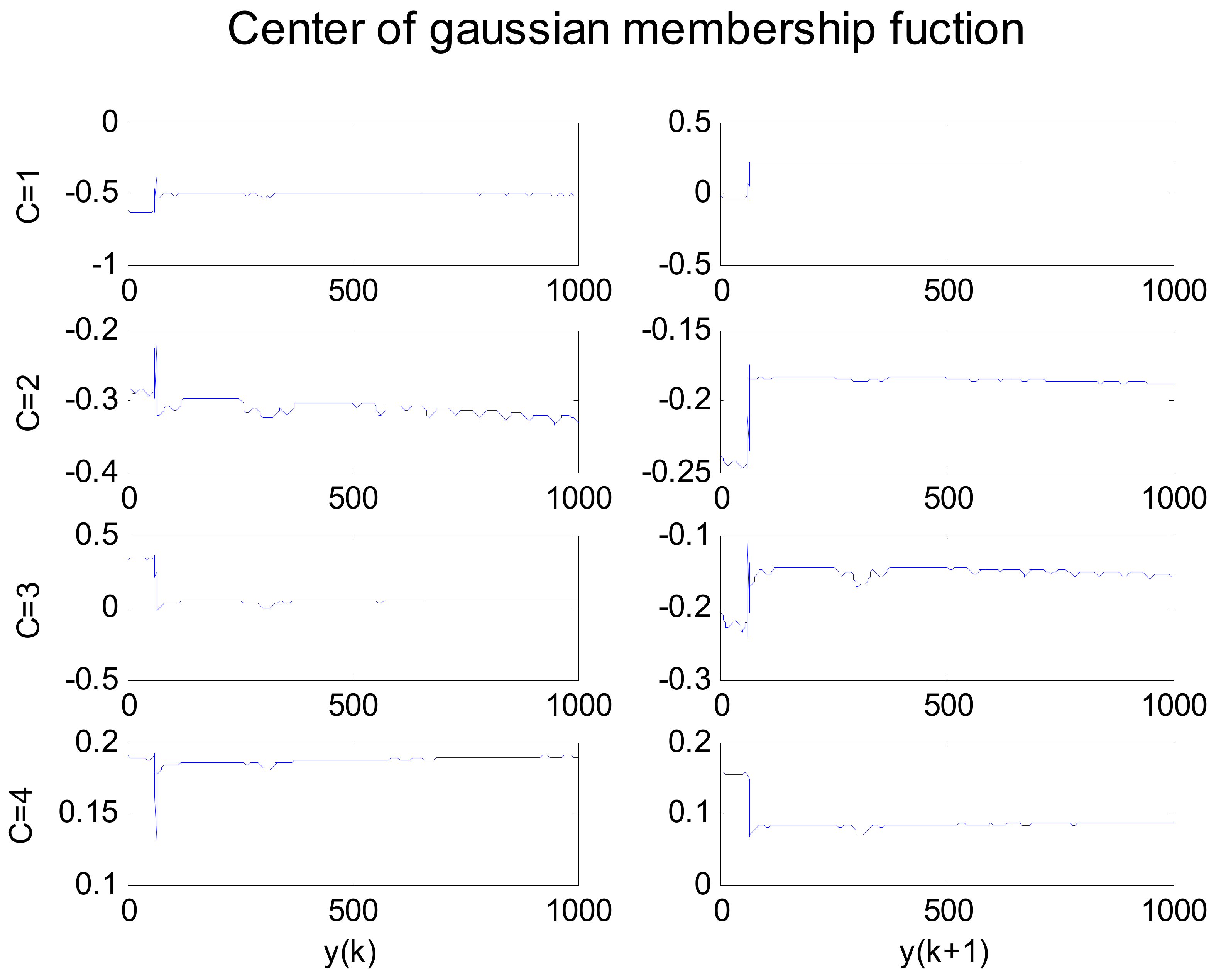
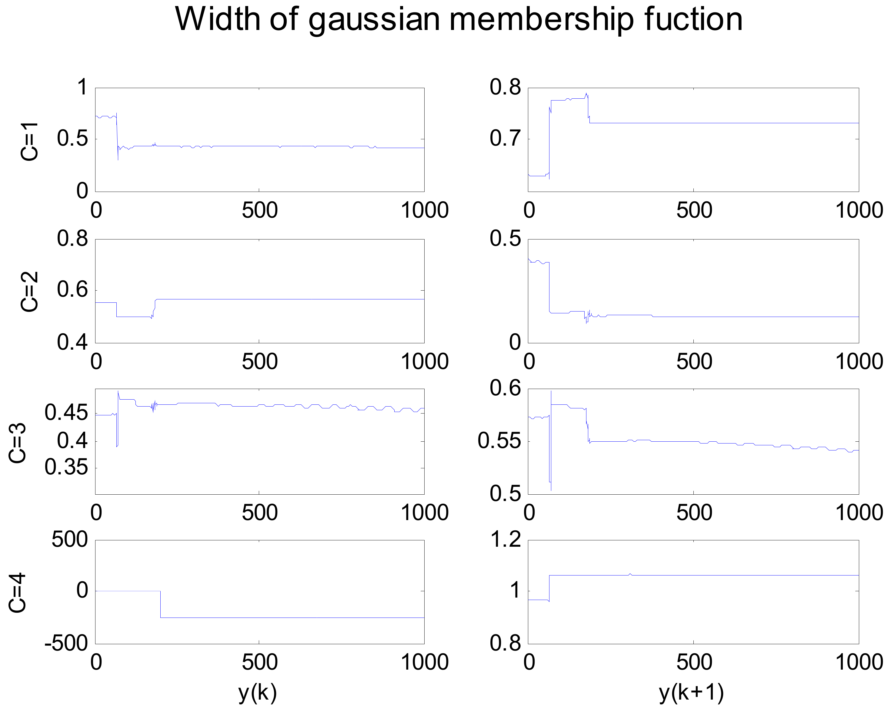
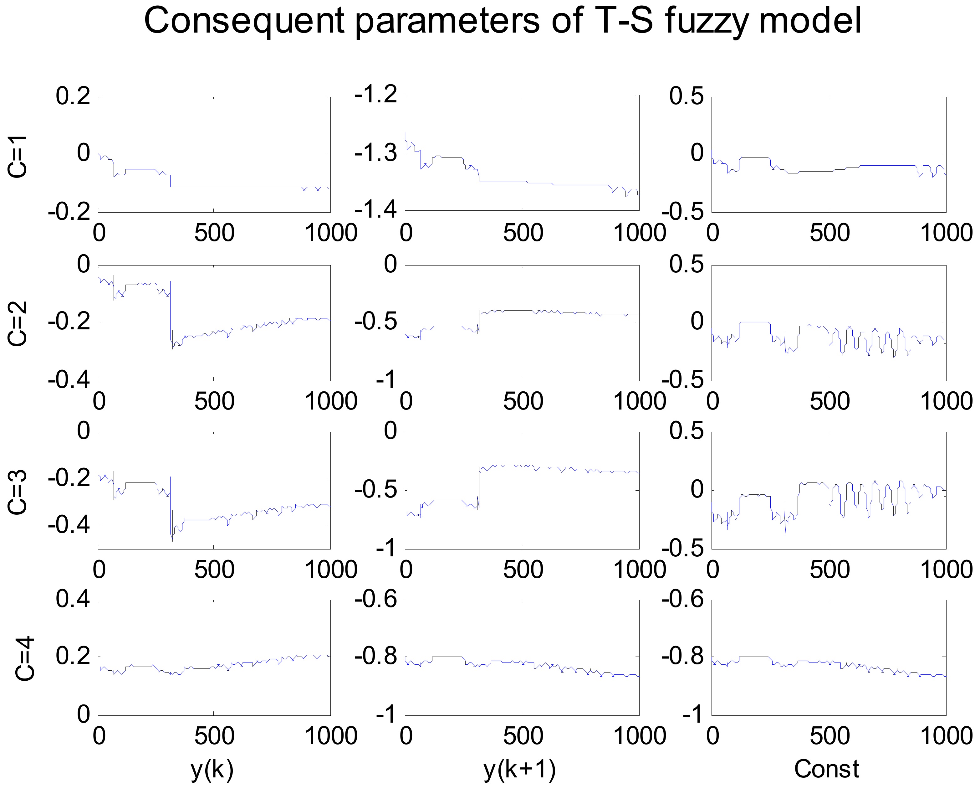
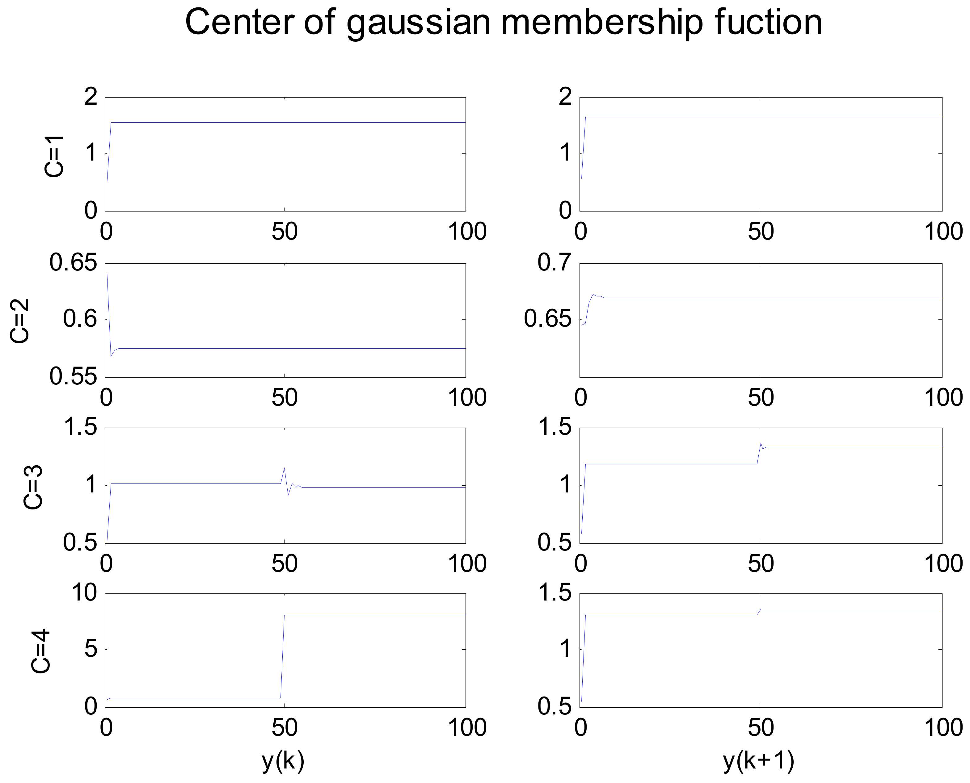
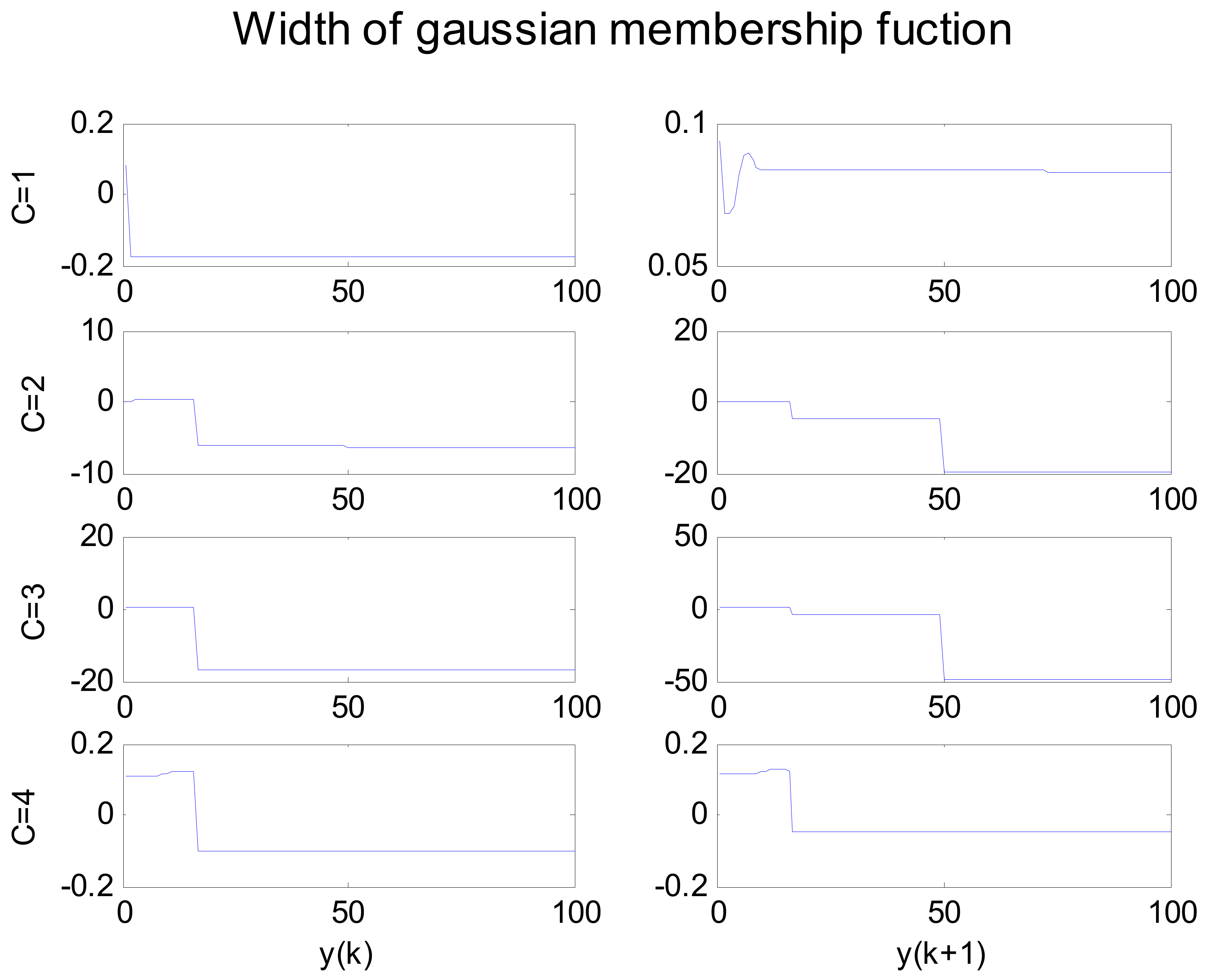
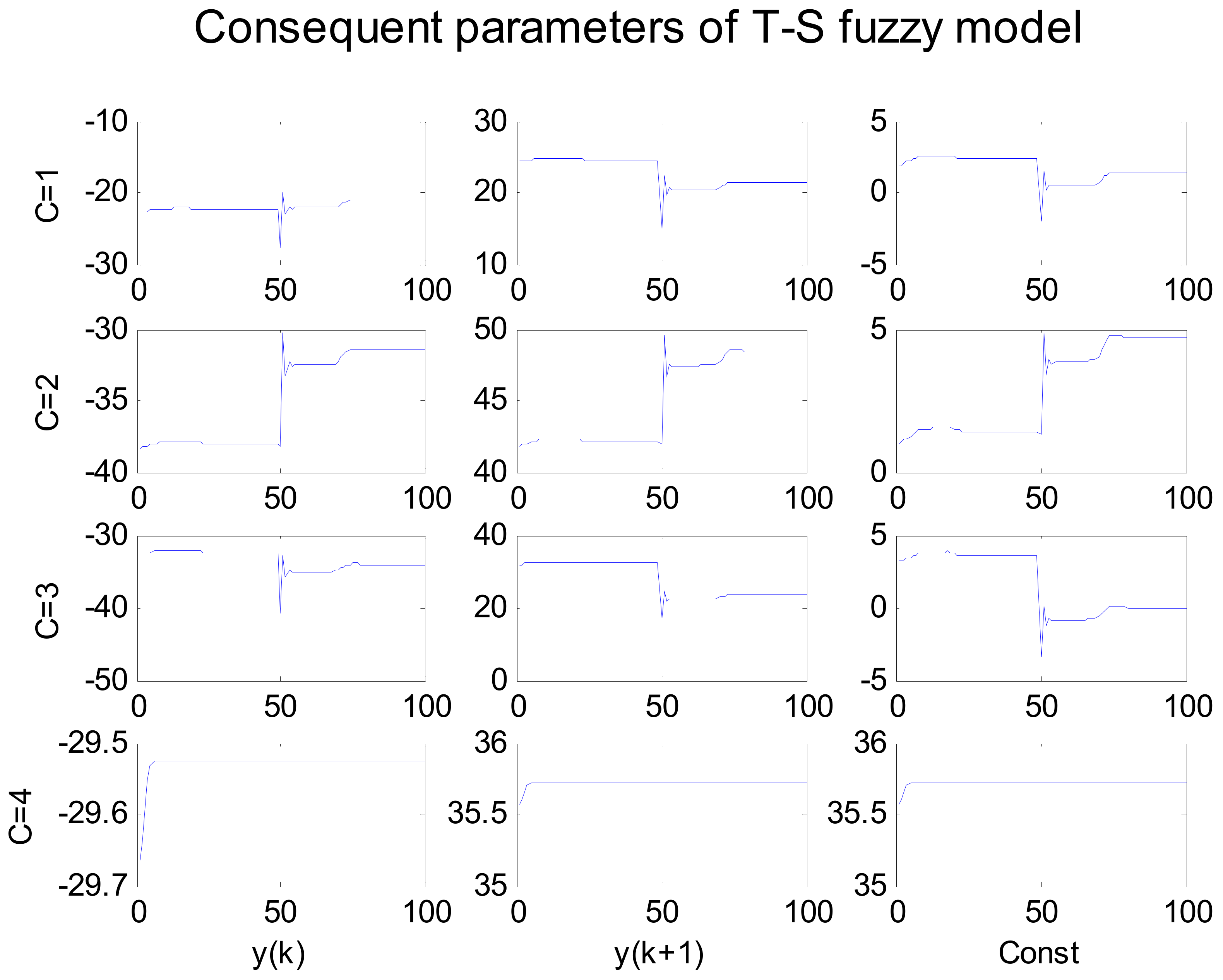
FCRM clustering is a local search algorithm, when it falls into local optimum, the algorithm will exit the iteration process. In order to ensure convergence of the method and get optimal parameters, online parameters adjustment was applied by the error of the system and desired output using the error back propagation training algorithm in this paper. When the error reaches the expected value, the adaptive inverse controller parameters will keep a constant value and reach optimization value, which can be seen from Figure 10, Figure 11 and Figure 12. Figure 10 shows the center curve of Gaussian membership function, Figure 11 shows the width curve of Gaussian membership function, and Figure 12 shows the consequent parameter curve of the T-S fuzzy model.

5.2. Simulation 2

In this simulation a liquid level control object of spherical container is considered, whose discretization equation is described as follows.

$$y(k+1)=y(k)+0.05\frac{u(k)-\sqrt{2g(y(k)-y_0}}{\pi R^2(1-(R^2-y(k)/R^2)}$$

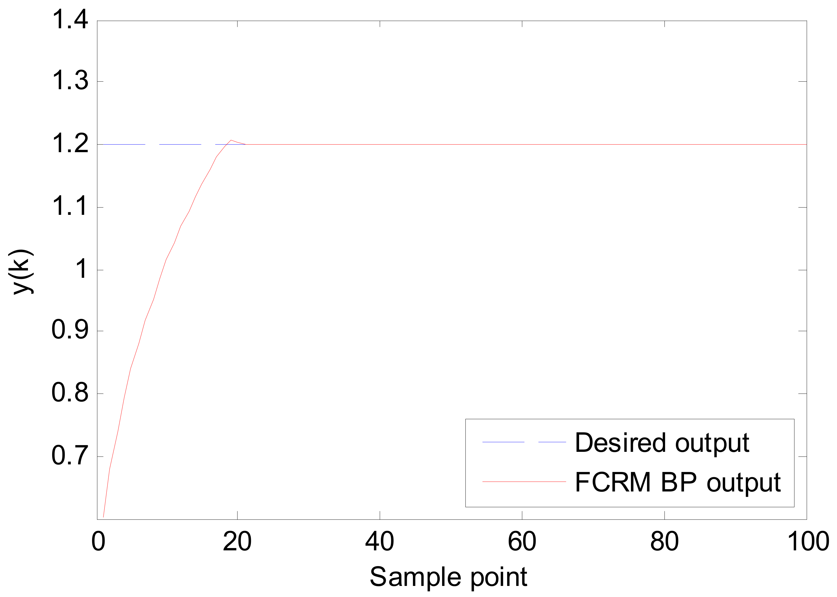
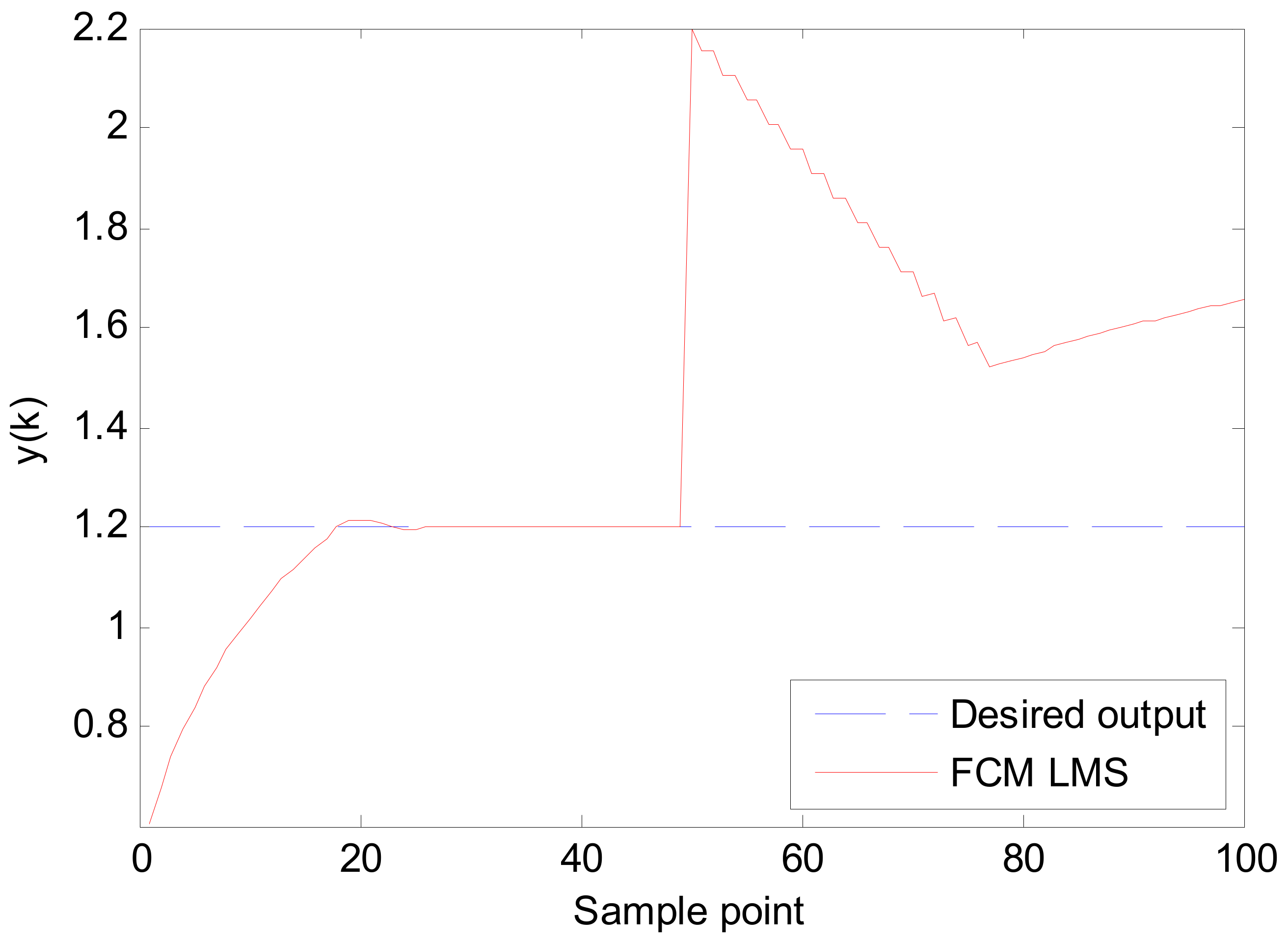
where g = 9.8 kg/N, y₀ = 0.1 m, R = 1 m, the initial liquid high is y(1) = 0.5 m, and the desired liquid high is 1.2 m.

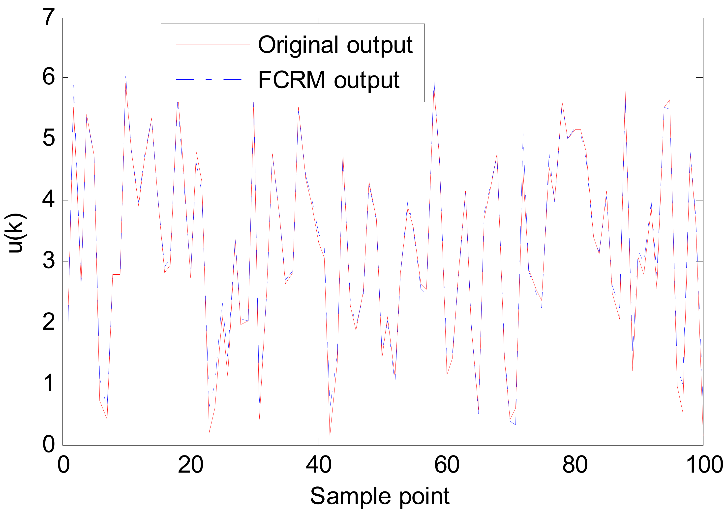
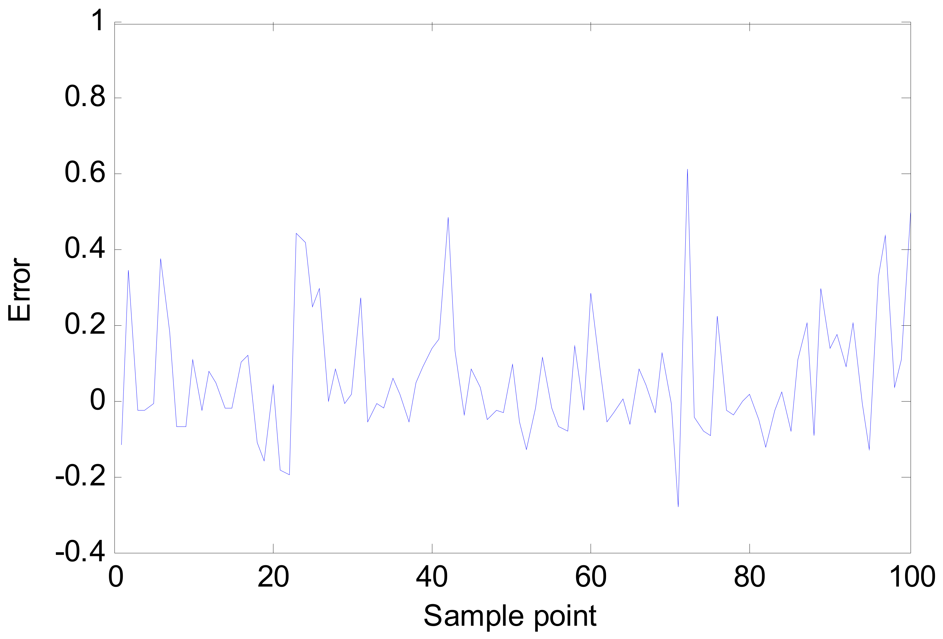
The positive model of the object is y(k + 1) = f(y(k),u(k)), so the inverse model is u(k) = g(y(k), y(k + 1)). Like simulation 1, the inverse model of the object is established by the FCRM clustering algorithm. Firstly, the random number with uniform distribution is produced as the input u(k) of the system in the interval [0, 6]. Through the object model, 100 input and output pairs are generated to establish the inverse model. The number of clustering (number of fuzzy rules) chosen in this case is 4, and in simulation 2, η_α = η_β = η_θ = 0.2. Figure 13 shows the output curve of the FCRM clustering logarithm inverse model and sample, and Figure 14 shows the errors.

Figure 15 shows that the response curves of system output and desired output. As can be seen from Figure 15, the system will reach the set value when the algorithm is simulated to 23 steps. The algorithm in [16] uses eight rules, and when the system reaches the set value, it is the 35th step.

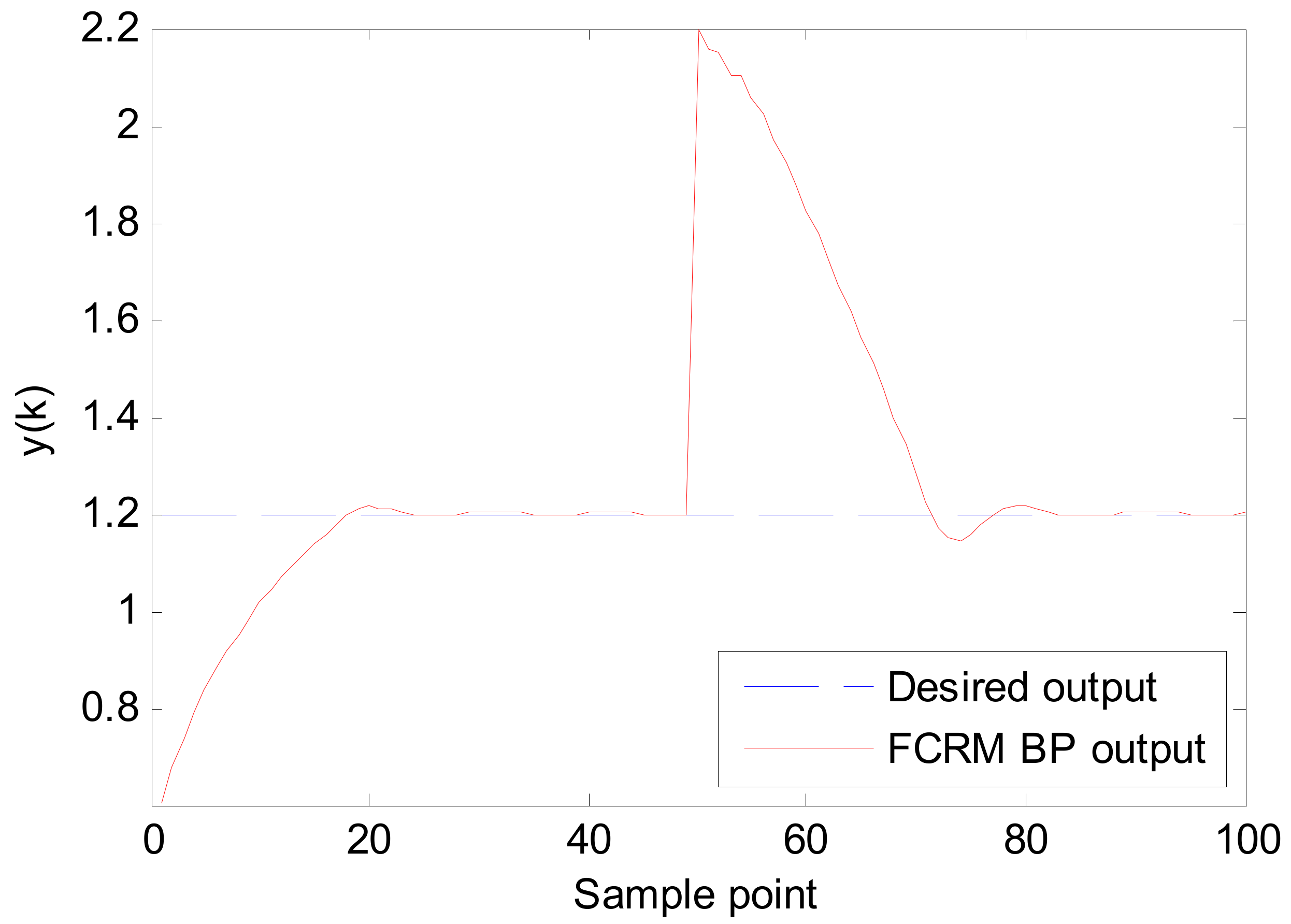
To illustrate the robustness of proposed adaptive inverse controller, when the simulation reaches 50 steps, a disturbance of 1 m is added to the system output. Figure 16 shows the response curve of the system output and the expected output when the disturbance is added.

Also, Figure 17 shows the center curve of the Gaussian membership function, Figure 18 shows the width curve of the Gaussian membership function, and Figure 19 shows the consequent parameter curve of the T-S fuzzy model for simulation 2.

In this simulation, the inverse controller based on the FCM clustering algorithm and LMS also adopts four fuzzy rules, and the system output becomes divergent, as shown in Figure 20.

In these 2 simulations, a fixed rate is adopted, and three parameters learning rates are the same. A potential research problem of this algorithm is how to decide learning rates of ${\alpha }_j^i$,${\beta }_j^i$, and ${\mathit{\theta }}_i$ when the parameters are adjusted online by the BP algorithm. In the future, variable and different learning rates will be researched to enhance the controller accuracy.

6. Conclusions

In accordance with the problem that it is difficult to get the inverse model mathematical expression of adaptive inverse controller, and LMS online parameter adjustment only adjusts the consequent parameters, we proposed an adaptive fuzzy inverse controller design method based on the FCRM and BP algorithm. The point-to-surface distance described by the FCRM clustering algorithm matches exactly the consequent form of the T-S fuzzy model, and the T-S fuzzy inverse model of the controlled object is established. The premise membership function of the T-S fuzzy model is Gaussian, and the BP algorithm is applied to adjust the center and width of the Gaussian membership function and the linear parameters of the consequent expression of T-S fuzzy model. By simulation, the tracking accuracy of the proposed adaptive inverse controller is higher than other inverse models, and the system stability can be maintained when the system output has disturbances.

References

- Yi, J.H.; Deb, S.; Dong, J.; Alavi, A.H.; Wang, G.G. An improved NSGA-III algorithm with adaptive mutation operator for big data optimization problems. Future Gener. Comput. Syst. 2018, 88, 571–585. [Google Scholar] [CrossRef]
- Wang, G.G.; Guo, L.; Gandomi, A.H.; Hao, G.S.; Wang, H. Chaotic krill herd algorithm. Inf. Sci. 2014, 274, 17–34. [Google Scholar] [CrossRef]
- Wang, G.G.; Gandomi, A.H.; Alavi, A.H. An effective krill herd algorithm with migration operator in biogeography-based optimization. Appl. Math. Model. 2014, 38, 2454–2462. [Google Scholar] [CrossRef]
- Wang, G.; Guo, L.; Wang, H.; Duan, H.; Liu, L.; Li, J. Incorporating mutation scheme into krill herd algorithm for global numerical optimization. Neural Comput. Appl. 2014, 24, 853–871. [Google Scholar] [CrossRef]
- Nino-Ruiz, E.D.; Ardila, C.; Capacho, R. Local search methods for the solution of implicit inverse problems. Soft Comput. 2018, 22, 4819–4832. [Google Scholar] [CrossRef]
- Nino-Ruiz, E.D.; Yang, X.S. Improved Tabu Search and Simulated Annealing methods for nonlinear data assimilation. Appl. Soft Comput. 2019. [Google Scholar] [CrossRef]
- De La Sen, M. On the robust adaptive stabilization of a class of nominally first-order hybrid systems. IEEE Trans. Autom. Control 1999, 44, 597–602. [Google Scholar] [CrossRef]
- Bilbao-Guillerna, A.; De la Sen, M.; Ibeas, A.; Alonso-Quesada, S. Robustly stable multiestimation scheme for adaptive control and identification with model reduction issues. Discret. Dyn. Nat. Soc. 2005, 2005, 31–67. [Google Scholar] [CrossRef]
- Yoo, S.J. Adaptive control of non-linearly parameterised pure-feedback systems. IET Control Theory Appl. 2012, 6, 467–473. [Google Scholar] [CrossRef]
- Widrow, B.; Walach, F. Adaptive Inverse Control; Prentice-Hall: Upper Saddle River, NJ, USA, 1996. [Google Scholar]
- Yingnong, D.; Chongzhao, H. Adaptive inverse control based on volterra polynomial basis function neural networks. J. Xi’an Jiao Tong Univ. 2000, 34, 8–12. [Google Scholar]
- Dang, Y.N.; Han, C.Z. Direct adaptive inverse control strategy based on modified VPBF neural networks. Control Decis. 2001, 16, 633–636. [Google Scholar]
- Hu, T.T.; Kang, B.; Shan, Y.N. Study on identification of adaptive inverse control system based on dynamic function linked neural network. Comput. Sci. 2017, 44, 203–208. [Google Scholar]
- Salman, R. Neural networks of adaptive inverse control systems. Applied Math. Comp. 2005, 163, 931–939. [Google Scholar] [CrossRef]
- Liu, F.C.; Liu, Y.; Dou, J.M.; Zhang, Y.-X. Model reference adaptive inverse control based on T-S fuzzy model. Syst. Eng. Electron. 2013, 35, 1940–1947. [Google Scholar]
- Liu, F.C.; Zhang, Y.X.; Wang, Y.J.; Dou, C. Adaptive inverse control method based on fuzzy inverse mode. Chin. J. Sci. Instrum. 2010, 31, 961–967. [Google Scholar]
- Ding, H.S.; Mao, J.Q.; Lin, Y. Adaptive direct inverse control based on fuzzy tree models. Acta Autom. Sin. 2008, 34, 574–580. [Google Scholar] [CrossRef]
- Gao, J.J.; Li, X.M.; Liu, Y.; Liu, F. Adaptive inverse control based on interval type 2 T-S fuzzy model. Fuzzy Syst. Math. 2016, 30, 59–73. [Google Scholar]
- Deng, L.C. Adaptive Inverse Control on Object of Superheated Steam Temperature for Boiler. Ph.D. Thesis, Chong Qing University, Chongqing, China, 2007. [Google Scholar]
- Chen, H.; Wang, G.J.; Wang, Z.J. Adaptive inverse control for feed water and superheated steam temperature of supercritical pressure boiler. J. Chongqing Univ. 2013, 36, 32–36. [Google Scholar]
- Kumbasar, T.; Eksin, I.; Guzelkaya, M.; Yesil, E. An inverse controller design method for interval type-2 fuzzy models. Soft Comput. 2015, 21, 1–22. [Google Scholar] [CrossRef]
- Wang, T.C.; Tong, S.C. Direct inverse control of cable-driven parallel system based on type-2 fuzzy systems. Inf. Sci. 2015, 310, 1–15. [Google Scholar] [CrossRef]
- Ulu, C. Exact Analytical Inversion of Interval Type-2 TSK Fuzzy Logic Systems with Closed Form Inference Methods. Appl. Soft Comput. 2015, 37, 60–70. [Google Scholar] [CrossRef]
- Liu, F.C.; Liu, Y.; Xu, W.L.; Liu, J. Fuzzy adaptive inverse control for pneumatic loading system. J. Mech. Eng. 2014, 50, 185–190. [Google Scholar] [CrossRef]
- Wang, T.; Tong, S.; Yi, J.; Li, H. Adaptive Inverse Control of Cable-Driven Parallel System Based on Type-2 Fuzzy Logic Systems. IEEE Trans. Fuzzy Syst. 2015, 23, 1803–1816. [Google Scholar] [CrossRef]
- Cheng-Dong, L.; Jian-Qiang, Y.; Yi, Y.; Dong-Bin, Z. Inverse Control of Cable-driven Parallel Mechanism Using Type-2 Fuzzy Neural Network. Acta Autom. Sin. 2010, 36, 459–464. [Google Scholar]
- Kumbasar, T.; Eksin, I.; Guzelkaya, M.; Yesil, E. Interval type-2 fuzzy inverse controller design in nonlinear IMC structure. Eng. Appl. Artif. Intell. 2011, 24, 996–1005. [Google Scholar] [CrossRef]
- Fallah, M.; Moetakef-Imani, B. Adaptive inverse control of chatter vibrations in internal turning operations. Mech. Syst. Signal Process. 2019, 129, 91–111. [Google Scholar] [CrossRef]
- Liu, F.C.; Gao, X.; Wu, S.C. Research on adaptive inverse control and its future developments. Chin. J. Sci. Instrum. 2008, 29, 2683–2688. [Google Scholar]
- Kumbasar, T.; Eksin, I.; Guzelkaya, M.; Yesil, E. Adaptive fuzzy model based inverse controller design using BB-BC optimization algorithm. Expert Syst. Appl. 2011, 38, 12356–12364. [Google Scholar] [CrossRef]
- Takagi, T.; Sugeno, M.; Sugeno, M. Fuzzy Identification of Systems and its Applications to Modeling and Control. IEEE Trans. Syst. Man Cybern. 1985, 15, 116–132. [Google Scholar] [CrossRef]
- Chen, J.Q.; Xi, Y.G.; Zhang, Z.J. A clustering algorithm for fuzzy model identification. Fuzzy Sets Syst. 1998, 98, 319–332. [Google Scholar] [CrossRef]
- Kung, C.C.; Su, J.Y. Affine Takagi-Sugeno fuzzy modelling algorithm by fuzzy c-regression models clustering with a novel cluster validity criterion. IET Control Theory Appl. 2007, 1, 1255–1265. [Google Scholar] [CrossRef]
- Li, C.; Zhou, J.; Xiang, X.; Li, Q.; An, X. T–S fuzzy model identification based on a novel fuzzy c-regression model clustering algorithm. Eng. Appl. Artif. Intell. 2009, 22, 646–653. [Google Scholar] [CrossRef]
Figure 1.
Fuzzy inverse modeling structure.