Article

A Fuzzy Technique for On-Line Aggregation of POIs from Social Media: Definition and Comparison with Off-Line Random-Forest Classifiers

Department of Management, Information and Production Engineering, University of Bergamo, Viale Marconi 5, I-24044 Dalmine, Italy
*
Author to whom correspondence should be addressed.
Submission received: 21 October 2019 / Revised: 29 November 2019 / Accepted: 3 December 2019 / Published: 7 December 2019
(This article belongs to the Section Information Applications)

Abstract

:
Social media represent an inexhaustible source of information concerning public places (also called points of interest (POIs)), provided by users. Several social media own and publish huge and independently-built corpora of data about public places which are not linked each other. An aggregated view of information concerning the same public place could be extremely useful, but social media are not immutable sources, thus the off-line approach adopted in all previous research works cannot provide up-to-date information in real time. In this work, we address the problem of on-line aggregating geo-located descriptors of public places provided by social media. The on-line approach makes impossible to adopt machine-learning (classification) techniques, trained on previously gathered data sets. We overcome the problem by adopting an approach based on fuzzy logic: we define a binary fuzzy relation, whose on-line evaluation allows for deciding if two public-place descriptors coming from different social media actually describe the same public place. We tested our technique on three data sets, describing public places in Manchester (UK), Genoa (Italy) and Stuttgart (Germany); the comparison with the off-line classification technique called “random forest” proved that our on-line technique obtains comparable results.

1. Introduction

In the last few years, social media have played an increasingly-important role as information sources for many categories of people (such as travelers, researchers, public administrators, company managers, and so on). In particular, the exploitation of information concerning public places (also called points of interests (POIs)) is continuously increasing: posts written by other people concerning public places (such as reviews) are becoming more and more important for decision making (for example, to decide whether to visit a museum).
Currently, several players own very large corpora of information concerning public places. Google has the corpus built for Google Maps; its service called Google Places is a valid tool to get lists of descriptors of public places in a given area. Facebook has a large corpus of pages concerning public places; pages are created by owners of places to promote their business (for example, restaurants, pubs, museums, and so on). Trip Advisor collects reviews about public places looked for by travelers (typically, restaurants, hotels, and so on). Other famous social media that collect information about public places are Yelp and FourSquares.
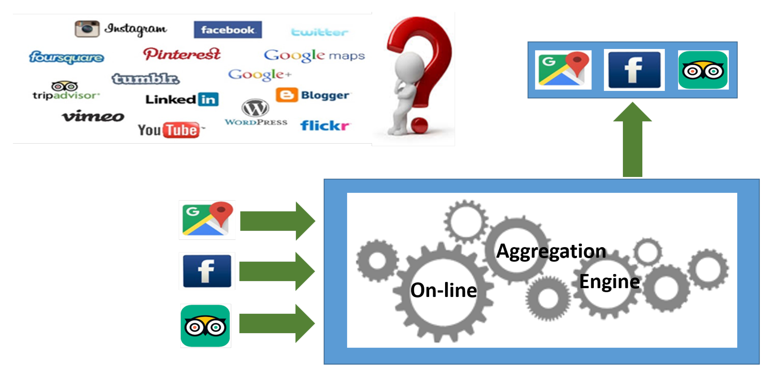
Usually, social media users who wish to get information concerning a given public place, start by exploiting one source of information (for example, Google Places) and one or two other social media (for example, Facebook and/or Trip Advisor). This activity is very tedious to carry on, in particular when a complete panorama about places in a given area is wished; in fact, at present, it can be performed only by aggregating information concerning the same place that comes from multiple sources by hand, by interacting with each single source. Clearly, an on-line aggregation engine for information describing public places would help people greatly.
Figure 1 illustrates the scenario. A user seeks for a public place in a given city, by getting a list of places provided by a system, for example Google Places; he/she chooses the desired one and asks the aggregation engine to provide all pieces of information concerning that place together (like news, events, reviews, and so on) from several sources (such as Facebook, Trip Advisor, and so on).
The on-line approach is necessary because on-line social media are not stable sources; as far as public places are concerned, information is continuously added, updated, and removed; therefore, the best way to aggregate up-to-date information is performing the aggregation on demand.
However, the social nature of social media requires dealing with an important issue: the same place could have a different name, address, and coordinates in the different sources. As an example, consider the following case taken from the area of Manchester (UK): the place with Facebook name “Al-Jumeirah”, in Google Places is named as “Al Jumeirah Restaurant”; to a human eye, they clearly appear to be the same, but this is not obvious for an automated algorithm.
In literature, this problem is usually called “geo-spatial data conflation” and it has been widely studied for off-line contexts, i.e., when lists of places are available in advance and can be analyzed and processed with time-consuming techniques. For example, [1,2,3] adopt some kind of learning technique to overcome the limitations of applying string-similarity measures. Even those works that propose methods based on string-similarity metrics evaluated on names and/or addresses, such as [4], do not consider coordinates of places, and some works [5,6] use complex geometries that are not available in our context. In general, the problem of on-line conflation of geographical data has not been considered. Section 2 provides an extensive analysis of the literature, that could help readers understand the research context.
The contribution of this paper is the definition and evaluation of a technique for on-line aggregating descriptors of public places coming from two different social media, without prior knowledge and off-line activities. We follow an approach based on fuzzy logic and possibility theory [7]: we propose a binary fuzzy relation, named M a t c h i n g P l a c e s , to compare two place descriptors; the membership degree of this relation describes the degree of likelihood that the two descriptors actually describe the same place. Note that, in literature, to the best of our knowledge fuzzy approaches for on-line conflation of geographical data have not been proposed; the only work based on a fuzzy technique that addresses a similar problem is [8], in which the authors consider data sets of generic objects (neither public places nor generic geographical objects).
In order to evaluate the goodness of the approach, the technique has been implemented within a prototype library. Then, we downloaded three data sets describing places in three different cities, such as Manchester (UK), Genoa (Italy), and Stuttgart (Germany): descriptors were downloaded from Google Places and paired with descriptors of Facebook pages. As a baseline for the evaluation, we considered our preliminary version of the binary fuzzy relation introduced in [9], showing that the new definition (proposed in this paper) significantly improves the effectiveness of the technique. Then, we make a comparison with a machine-learning technique, named “random forest”: it is a well known classification technique, to be executed off-line. We will show that our technique obtains comparable results, even though it can be applied on-line, without a preliminary download of the data sets.
The paper is organized as follows. Section 2 discusses related works. Section 3 presents the problem and the technique we propose. Section 4 introduces the formal fuzzy framework exploited in Section 5 to define the binary fuzzy relation named M a t c h i n g P l a c e s . Section 6 presents how we evaluated the technique, in particular how we built the data sets and the comparison with the baseline and with random forest classifiers. Finally, Section 7 draws the conclusions and future developments.

2. Related Works

Social media have become very important tools for people, not only for exchanging messages concerning their private life, but also for finding information concerning public places. In fact, both owners and visitors of public places can post messages either promoting events or disseminating opinions somehow concerning the place. Contemporary citizens rely on social media to experience the city. The work [10] is an interesting study, that helps to understand how people live their cities, in particular how they live public places by exploiting location-based services. The paper points out limitations to flexibly and effectively use them by citizens.
Clearly, the need to aggregate information concerning public places is not new and several works were published on the topic. However, we observed that previous works usually do not exploit coordinates (latitude and longitude) to conflate descriptors of the same public place; at the best of our knowledge, only the technique proposed by [11] considers coordinates and distance. Moreover, all of them adopt an off-line approach: corpora containing data describing public places must be previously downloaded and then aggregated. This approach is suitable for stable and verified data sets. For instance, digital gazetteers are examples of stable and verified data sets describing places [5]. This work jointly adopts three metrics that evaluate shape similarity (because it is argued that place markers are not enough), type similarity (or category of places) and names, trying to reproduce the cognitive approach performed by people. Our work approaches the problem in a similar way; however, we can rely neither on shapes of places (social media provide markers only) nor on reliable categories (social media adopt specific and not comparable categories).
Nevertheless, the topic of aggregating information about public places or POIs coming from social media is current; in fact, many researchers are working on this topic. For example, the work [12] addresses semantic aligning of heterogeneous geo-spatial data sets (GDs) produced by various organizations, in order to find an efficient similarity matching technique. This work seems to be related to our work; in fact, to solve the aligning problem, the authors presented a holistic approach to adapt the geo-spatial entities (concepts, properties and instances) together. In particular, they faced the problem of aligning the instances of various category systems by simultaneously matching unbalanced schema of data composed by multi-dimensional information.
The work [4] evaluates the DAS technique: it is based on an interesting word similarity measure, that is exploited in a three step process. Specifically, given the strings reporting names of two public places, they are compared (after removing blanks) as a whole (this is the word-similarity measure) and, after tokenization, as sentences (this is called the sentence-similarity measure); finally, if the two above-mentioned similarity measures are greater than a given threshold, a final comparison is made, where all characters in the strings are compared (this is called name-similarity measure). Although it is effective, the technique considers only names of public places, without considering coordinates.
The work by Santos et al. [1] is closely related to our work. The authors applied different string similarity metrics, as well as various machine learning methods, to solve the problem of toponym matching, in order to perform a comparative performance study. They show that machine learning methods outperform similarity metrics: in particular, classifiers based on the random forest method outperform other machine learning techniques. In our work, we show that it is possible to perform similarly to random forest classifiers, by combining similarity between names, addresses, and locations.
The work [3] addresses the problem of urban neighborhood identification. In particular, neighborhoods are regions (or areas) that own similar characteristics, whose names are often given by people that inhabit them. These names are important for people that live in these urban neighborhoods, because they constitute the socio-demographic identity of people; therefore, often they are not listed in official data sets. The source of information considered in [3] is the Craigslist platform (https://www.craigslist.org): specifically, ads concerning house rentals are of interest, because they are geo-tagged and contain neighborhood names. The methodology proposed by the authors extracts all n-grams from ads text and geo-tags them with coordinates associated with ads; then, a pool of statistical measures, possibly denoting spatial correlation, are associated to n-grams; these are labeled based on the capability of identifying neighbourhoods; finally, a random-forest classifier is built, in order to identify novel neighbourhoods. Interestingly, the paper shows that a classification model built on n-grams collected for Washington D.C. (USA), is able to discover n-grams denoting unknown neighborhoods in ads for Seattle, WA (USA) and Montreal, QC (CA), by using spatial statistical correlation measures associated with n-grams.
The authors of [13] address the problem of geo-spatial data conflation as well; in particular, they consider POIs, because they convey important information about spatial entities and territories. They propose a method to match objects (describing POIs) coming from different sources, by means of an entropy-based technique organized in four steps. (1) A normalized similarity formula is developed, that helps to simplify the computation of spatial attribute similarity; in particular, the authors specified the rule of attribution selection, then study POI matching for spatial, name, and category attribution and indicated a way for weighted multi-attribute matching of POIs. (2) They used phonetic and word segmentation methods in order to remove linguistic ambiguity. (3) They established category mapping in order to address heterogeneity among various classifications. (4) They calculated attribute weights by computing the entropy of attributes, in order to manage non-linearity of attribute similarity. Experiments demonstrated that this technique obtains good results in terms of precision and recall for matching instances from various POI data sets.
In another work [2] the authors face the problem of toponym matching by using a deep neural network. The focus is pairing strings that represent the same POI location. The authors noted that techniques based on string similarity metrics are either dedicated for matching POI names or combined with other metrics. But these techniques, that establish similarity by detecting common sub-strings, do not always detect the character substitutions involved in toponym changes caused by changes in language. Therefore, the authors present a matching approach based on a deep neural network in order to classify pairs of toponyms as “same POI” (matching) or “different POIs” (non matching). In particular, their network architecture exploits recurrent nodes in order to create representations from the sequences of bytes that are the strings to match. In a second step, the above representations are combined and passed to feed-forward nodes in order to achieve the classification decision. The authors used a data set of the GeoNames gazetteer. The final results show that their technique can do better than individual similarity metrics and methods based on supervised machine learning methods.
In [8], Bunke et al. do not focus on conflation of public places, but on conflation of objects from generic data sets. Specifically, they propose an approach based on fuzzy sets and fuzzy rules. In details, objects are seen as vectors of features; fuzzy sets are used to characterize the distance of each single pair of homogeneous features; fuzzy rules combine fuzzy sets evaluated on single feature pairs and determine the distance between two objects. At the best of our knowledge, this is the closest proposal to our work, since it adopts a fuzzy approach, although it does not consider coordinates.
A side problem is addressed in [6]: Jung et al. faced the problem of conflating geographical objects from different catalogues coming from different portal APIs (Application Programming Interfaces). Although apparently it is similar to the problem addressed in this paper, the problem they addressed is quite different, because they consider the shape of objects and the neighborhoods of them on the map; in contrast, we consider punctual coordinates of public places, for which the shape of buildings is not available.
Fuzzy approaches and soft computing are of interest in many contexts, in particular to manage web data and geographical information. To cite some work related to our experience, in [14,15,16] fuzzy techniques to perform location-based spatial queries are presented; fuzzy logic helps in dealing with uncertainty about both user position and places of interest. The methodology presented in these papers is also the long-term result of research in flexible querying in relational databases: in fact, an extension to SQL, called SoftSQL, was proposed to provide users of relational databases with a powerful tool to express queries based on linguistic predicates and soft aggregators on relational tables [17,18].
To conclude, soft approaches can be applied to post-process web searches; in [19,20,21] we studied the evolution of a framework for clustering web-search results; clusters could be manipulated, in order to find out the pool of search results that fit user needs. The soft approach was essential to deal with imprecision of search results.

3. Problem Statement

In this section, we state the problem we address in this paper. To do that, we need to introduce the concept of place descriptor.
Definition 1.
Place descriptor. A place descriptor is a tuple
p d = n a m e , a d d r e s s , c i t y , l o c a t i o n : l a t i t u d e , l o n g i t u d e
where the names of fields clearly denote their meaning; notice that latitude and longitude are nested within a compound field named l o c a t i o n .
If a string-valued field ( n a m e and a d r e s s ) is missing, its value is the zero-length string; if a number-valued field ( l a t i t u d e and l o n g i t u d e ) is missing, it has the n u l l value.
The general problem we want to address is to develop a software library that, given a place descriptor, looks for descriptors of the same place in social media.
To achieve this goal, the following essential activities must be performed:
  • Given the descriptor p d 1 of a place obtained from source S 1 , a request must be sent to APIs of source S 2 ;
  • The set D 2 = { p d 2 , 1 , , p d 2 , n } of descriptors obtained from source S 2 possibly matching p d 1 must be built.
  • Problem 1, hereafter presented, must be solved.
Problem 1.
Consider a place descriptor p d 1 obtained from a source S 1 and the set D 2 = { p d 2 , 1 , , p d 2 , n } of place descriptors p d 2 , i obtained from a source S 2 and possibly matching   p d 1 .
The problem we address in this paper is the following: given p d 1 and D 2 , find the descriptor p d 2 ¯ D 2 that actually describes the same place described by p d 1 , if any. p d 2 ¯ must be identified by means of a ranking method that can be applied without any prior knowledge and without any off-line activity.
Problem 1 is addressed in Section 5 by adopting a fuzzy-logic approach, that relies on possibility theory [7]. Consequently, Section 4 introduces basic concepts about fuzzy relations.

4. Concepts about Fuzzy Relations

Fuzzy logic has been introduced by [22] and its goal is to represent the world in terms of non-precise (fuzzy) concepts. To this end, fuzzy logic provides the possibility of defining gradual concepts, i.e., concepts that are not only true or false, but partially true. Classical logical operators have been redefined, as well as a plethora of aggregation operators have been defined, consequently.
In this formal framework, predicates become linguistic predicates, i.e., they express soft linguistic concepts and relations (see the works [23,24]).

4.1. Basic Concepts

Hereafter, we introduce basic concepts, that will be exploited in the rest of the paper.
Definition 2.
Binary fuzzy relation and membership degree. Consider a binary relation R between two items e 1 ad e 2 . The membership degree μ R ( e 1 , e 2 ) [ 0 , 1 ] expresses the degree with which the pair e 1 , e 2 belongs to relation R (or, alternatively, the degree with which relation R is satisfied for the e 1 , e 2 pair). In particular, if μ R ( e 1 , e 2 ) = 1 , this means that the e 1 , e 2 pair fully belongs to relation R (i.e., relation R is fully satisfied by the e 1 , e 2 pair)); if μ R ( e 1 , e 2 ) = 0 , this means that the e 1 , e 2 pair does not belong to relation R (i.e., relation R does not hold at all for the e 1 , e 2 pair); an intermediate value means that the e 1 , e 2 pair partially belongs to relation R (i.e., relation R partially holds for the e 1 , e 2 pair).
For example, suppose we want to define the C o m p a r a b l e S h o p s ( c 1 , c 2 ) relation between two cities c 1 and c 2 , that compares cities c 1 amd c 2 based on the respective number of shops c 1 . s h o p s and c 2 . s h o p s . The following ratio:
r s = | c 1 . s h o p s c 2 . s h o p s | m a x ( c 1 . s h o p s , c 2 . s h o p s )
is the percentage of the difference between the shops divided by the higher number of shops. We might define μ C o m p a r a b l e S h o p s ( c 1 , c 2 ) , the membership degree of relation C o m p a r a b l e S h o p s , in this way:
  • if r s 0.1 , then μ C o m p a r a b l e S h o p s ( c 1 , c 2 ) = 1 , i.e., if the ratio is less than or equal to 10%, the two cities have a comparable number of shops;
  • if 0.1 < r s < 0.5 , then μ C o m p a r a b l e S h o p s ( c 1 , c 2 ) progressively decreases from 1 to 0, i.e., a value μ C o m p a r a b l e S h o p s ( c 1 , c 2 ) = 0.6 means that the number of shops is only partially comparable;
  • if r s 0.5 , than μ C o m p a r a b l e S h o p s ( c 1 , c 2 ) = 0 , i.e., the number of shops is not at all comparable.
Notice that, this way, we can express a linguistic predicate (i.e., comparable shops) as a fuzzy relation. The membership function gives the extent to which two cities have a comparable number of shops.
Fuzzy relations can be composed to express compound relations. To this end, the classical logical operators are extended; furthermore, various aggregation operators were proposed in literature [25].
Given two fuzzy terms t 1 and t 2 (we consider only relations as fuzzy terms), each one provided with its membership degree μ ( t 1 ) and μ ( t 2 ) , the operators A N D , O R and N O T are defined as follows (see [22]):
  • t 1 A N D t 2 has μ ( t 1 A N D t 2 ) = m i n ( μ ( t 1 ) , μ ( t 2 ) ) as membership degree;
  • t 1 O R t 2 has μ ( t 1 O R t 2 ) = m a x ( μ ( t 1 ) , μ ( t 2 ) ) as membership degree;
  • N O T t has μ ( N O T t ) = 1 μ ( t ) as membership degree.
In this paper, we make use of the weighted averaging operator (see Definition 2.1 in [25]) in the binary form w a β ( t 1 , t 2 ) . This operator weights the relative importance of two terms t 1 and t 2 , provided a weighting parameter β [ 0 , 1 ] that expresses the relative importance of term t 1 with respect to term t 2 . The membership degree is defined as μ ( w a β ( t 1 , t 2 ) ) = β × μ ( t 1 ) + ( 1 β ) × μ ( t 2 ) ) (when β = 0.5 the resulting membership degree is the average of membership degrees of terms t 1 and t 2 ).

4.2. Geographical Fuzzy Relation

Here, we define a geographical fuzzy relation whose aim is to define linguistic predicates that express the concept of “closeness” between two locations. A location l = l a t i t u d e , l o n g i t u d e is the pair of latitude and longitude (spherical coordinates) of a place.
Definition 3.
Close Relation. Consider two locations l 1 and l 2 , and function d i s t ( l 1 , l 2 ) that gives the geodetic distance, in meters, between l 1 and l 2 . The C l o s e ( l 1 , l 2 ) relation denotes how much the two locations are close each other. Given a minimum threshold m i n d and a maximum threshold m a x d , its membership function is defined as follows.
μ C l o s e ( l 1 , l 2 ) = { 1 i f 0 d i s t ( l 1 , l 2 ) m i n d ( m a x d d i s t ( l 1 , l 2 ) ( m a x d m i n d ) i f m i n d < d i s t ( l 1 , l 2 ) < m a x d 0 i f d i s t d ( l 1 , l 2 ) m a x d
Figure 2 depicts the membership function for the Close relation, with m i n d = 50 m and m a x d = 1000 m.
The rationale is that when two locations are at a distance less than 50 m, they are actually close. When the distance increases, the two locations become less and less close. After 1000 m, the membership degree is eventually 0, because the two locations can no longer be considered close.

4.3. Fuzzy Relation between Strings

Fuzzy relations can be used to compare strings as well. Clearly, the membership degree should be 1 when the two compared strings coincide; the membership degree should be 0 when the two compared strings are completely different; the membership degree should be an intermediate value between 0 and 1 when the two compared strings are similar but not equal.
We decided to adopt the Jaro–Winkler similarity measure, that currently is considered one of the best string-similarity measures. Since it is defined in the range [ 0 , 1 ] , it can be considered as the membership degree of a fuzzy relation to compare strings.
The Jaro–Winkler similarity measure is derived from the Jaro similarity measure (see the seminal paper [26], later cited in [27]), that is defined in the range [ 0 , 1 ] too; consequently, it can be considered as the membership function of another string-similarity relation. For this reason, we report both the definitions of Jaro and Winkler string-similarity relations.
Definition 4.
Jaro String–Similarity Relation. The Jaro string-similarity relation is applied to a pair of strings s 1 and s 2 , i.e., J a r o ( s 1 , s 2 ) . Its membership function μ J a r o ( s 1 , s 2 ) is defined as:
μ J a r o ( s 1 , s 2 ) = { 0 i f   m = 0 1 3 m | s 1 | + m | s 2 | + m t m o t h e r w i s e
where | s 1 | and | s 2 | are the lengths of strings s 1 and s 2 (respectively), m is the number of matching characters and t is half the number of transpositions of characters.
Terms m and t are obtained by comparing each character in s 1 with each character in s 2 , in order to find matching characters. Two characters in the two strings are considered matching if they are the same and their positions are no farther than
g r e a t e s t m a x ( | s 1 | , | s 2 | ) 2 1
where function g r e a t e s t is the greatest integer number less than or equal to the argument.
With this premise, m is the number of matching characters that maintain the order, while t is the number of matching characters that do not respect the order divided by 2.
In [28], Winkler proposed a measure that is based on Jaro’s measure, in order to consider common prefixes. Hereafter, we define the fuzzy relation named Winkler, based on Winkler’s string-similarity measure.
Definition 5.
Winkler String-Similarity Relation. The Winkler string-similarity relation is applied to a pair of strings s 1 and s 2 , i.e., W i n k l e r ( s 1 , s 2 ) . Its membership function μ W i n k l e r ( s 1 , s 2 ) is defined as:
μ W i n k l e r ( s 1 , s 2 ) = μ J a r o ( s 1 , s 2 ) + l × p × ( 1 μ J a r o ( s 1 , s 2 ) )
where l is the length of the longest common prefix at the beginning of the strings up to a maximum of four characters; p is a constant scaling factor (usually, p = 0.1 ).
Recall that Jaro–Winkler is a similarity measure; we use it as the membership function of the Winkler relation. In any case, the Winkler relation is not a fuzzy logic operator; thus, no specific properties like transitivity can be proven on it.

5. A Fuzzy Approach to Identify Matching Places

In this section, we present the fuzzy approach we followed to identify matching places and solve Problem 1. First of all, we introduce the general approach based on possibility theory. Then, we report the baseline solution which this work starts from. Finally, we present the novel proposal that is one of the main contributions of this paper.

5.1. Approach

In order to address Problem 1, we adopt an approach based on fuzzy logic and possibility theory, introduced by Zadeh in [7]. Hereafter, we explain the approach, considering our problem.
  • In our context, we have neither prior knowledge nor previous data sets; thus, machine learning techniques cannot be applied.
  • We try to tackle the problem by defining a binary fuzzy relation denoted as M a t c h i n g P l a c e s ( p d 1 , p d 2 ) on two place descriptors p d 1 ad p d 2 . Its role is to guess the degree of likelihood that the two descriptors p d 1 and p d 2 actually describe the same place. In other words, this relation expresses the possibility that p d 1 and p d 2 describe the same place, through its membership function.
  • The membership function of the M a t c h i n g P l a c e s relation expresses the degree of truth we give to the fact that descriptors p d 1 and p d 2 describe the same place. Based on this membership degree, we decide if they do actually match or do not, by de-fuzzifying: a pair with a membership degree no less than a given threshold α is considered as a “Good Pair”, otherwise as a “Bad Pair”.
  • In case for the same descriptor p d 1 more than one good pair is found (see Problem 1), the pair with the highest membership degree is chosen.
Hereafter, we explain the rationale behind the approach. The membership function of the M a t c h i n g P l a c e s ( p d 1 , p d 2 ) relation provides the degree of truth that two descriptors p d 1 and p d 2 actually match, i.e., that they describe the same place. By means of this degree of truth, we try to determine something that we do not know in advance, i.e., if the two descriptors match. In fact, reality is crisp (i.e., descriptors either do describe the same place or they do not). However, we do not know in advance the real situation, thus the membership degree is the degree of truth that we can suppose by comparing properties of descriptors: the greater the degree of truth, the greater the likelihood that the two descriptors describe the same place.
However, at the end we have to choose, i.e., we have to de-fuzzify. Given a threshold α , we assign a label to the p d 1 , p d 2 pair: the label is “Good Pair” (or simply “Good”) if the membership degree of the M a t c h i n g P l a c e s relation is no less than α ; otherwise, the label is “Bad Pair” (or simply “Bad”). The former label means that we suppose that descriptors p d 1 and p d 2 describe the same place; the latter means the contrary.
Thus, Problem 1 reduces to find a good formulation for the M a t c h i n g P l a c e s fuzzy relation and a proper value for the α threshold.
Note that we cannot rely on probability, because we do not have any prior knowledge about the actual situation; we get two descriptors, by on-line querying two social media, and we have to make a hypothesis. For this reason, we decided to rely on possibility theory.

5.2. Baseline Formulation for the MatchingPlaces Relation

The main focus of the research is to find the proper formulation for the M a t c h i n g P l a c e s fuzzy relation, that evaluates if two place descriptors actually describe the same place. In [9], we introduced a formulation, that we report in the following definition. This formulation, hereafter denoted as M a t c h i n g P l a c e s V 1 , constitutes our baseline.
Definition 6.
Relation M a t c h i n g P l a c e s V 1 ( p d 1 , p d 2 ) is defined as
M a t c h i n g P l a c e s V 1 ( p d 1 , p d 2 ) = = w a 0.5 ( w a 0.5 ( W i n k l e r ( p d 1 . a d d r e s s , p d 2 . a d d r e s s ) , C l o s e ( p d 1 . l o c a t i o n , p d 2 . l o c a t i o n ) ) , W i n k l e r ( p d 1 . n a m e , p d 2 . n a m e ) )
where the C l o s e relation is composed with the W i n k l e r relation on addresses, through the weighted averaging operator with weight 0.5 ; the resulting term is further composed with the W i n k l e r relation on names, again through the weighted averaging operator with weight 0.5 .
The membership function μ M a t c h i n g P l a c e s V 1 ( p d 1 , p d 2 ) is then defined as
μ M a t c h i n g P l a c e s V 1 ( p d 1 , p d 2 ) = = 0.5 × ( 0.5 × μ W i n k l e r ( p d 1 . a d d r e s s , p d 2 . a d d r e s s ) + 0.5 × μ C l o s e ( p d 1 . l o c a t i o n , p d 2 . l o c a t i o n ) ) + 0.5 × μ W i n k l e r ( p d 1 . n a m e , p d 2 . n a m e ) )
The Close relation, that estimates if two locations can be actually considered as “close”, is compounded with the Winkler relation on addresses: in this way, the contribution of geographic information has a higher priority with respect to information concerning names. In fact, the similarity between names is used to give the final contribution to geographical similarity: if two places are close and they have the same name, it is likely that they are the same place; if two places are close but their names are different, they are not the same place (probably, they are in the same building).
In [9], we tested the effectiveness of this relation with a threshold α = 0.75 and with thresholds m i n d = 100 m and m a x d = 2000 m for the C l o s e relation. We obtained good results, but the data set used during the experiments was clean: no descriptors with missing fields were present. In contrast, social media APIs can provide descriptors with missing fields; furthermore, we observed that Winkler’s string-similarity measure behaves properly with English addresses (where urban designations, such as “street” and “square”, are at the end), while it is in troubles with languages like Italian (where urban designations are at the beginning). For this reason, we decided to change the formulation of the M a t c h i n g P l a c e s relation, as described in the next section.

5.3. Novel Formulation for the MatchingPlaces Relation (Rewritten)

Social media APIs often provide descriptors that present various problems, in order to be effectively used for matching places. Hereafter, we report them.
  • Missing fields. Incomplete descriptors are often provided by social media APIs: this is due to the freedom given to users, who can upload incomplete information concerning places.
  • Contradictory information. Errors during input of information concerning places can occur, resulting in contradictions.
  • Different addresses for the same building. When a place is located in a building that can be easily seen by a main street/road but its (official) entrance is located in a secondary street, place owners prefer to provide the main street as address, instead of the official one. This makes it more complicated to match the same place.
  • District vs. city. Often, social media APIs provide the name of the city district for field c i t y in descriptors, instead of the actual city name. Without previous knowledge providing the set of districts in a given city, this behaviour prevents to use city names for matching places.
Based on the above-mentioned considerations, we have defined a new version of the M a t c h i n g P l a c e s relation, that in the remainder of the paper we denote as M a t c h i n g P l a c e s V 2 . We cannot define it immediately, because we need to introduce a fundamental relation named S a m e L o c a t i o n in Definition 13. However, since this relation must deal with possibly missing addresses and coordinates, its definition is not trivial. So first, we need to introduce some utility fuzzy relations and a utility function in Section 5.3.1. Then, in Section 5.3.2, we will define three sub-relations that separately deal with three different sub-cases concerning the possibility that two descriptors denote the same location; these three sub-relations will be aggregated into the global S a m e L o c a t i o n relation in Definition 13. Finally, in Section 5.3.3 Definition 14 presents the new formulation of the M a t c h i n g P l a c e s relation, denoted as M a t c h i n g P l a c e s V 2 .

5.3.1. Utility Relations and Functions

In this section, we introduce some utility relations and one utility function that will be used in Section 5.3.2.
Definition 7.
MissingStringRelation. The M i s s i n g S t r i n g ( s 1 , s 2 ) relation models a crisp situation, i.e., if the length of at least one of the two string arguments s 1 and s 2 is zero or not. It is defined as M i s s i n g S t r i n g ( s 1 , s 2 ) = N O T ( | s 1 | > 0 ) O R N O T ( | s 2 | > 0 ) . Its membership function results as μ M i s s i n g S t r i n g ( s 1 , s 2 ) = m a x ( 1 μ ( | s 1 | > 0 ) , 1 μ ( | s 2 | > 0 ) ) , where, given a comparison predicate p, μ ( p ) = 1 if p is true, otherwise μ ( p ) = 0 .
Definition 8.
MissingCoordsRelation. The M i s s i n g C o o r d s ( l 1 , l 2 ) relation models the case where one or more coordinates in the two location arguments are missing. It is defined as
M i s s i n g C o o r d s ( l 1 , l 2 ) = = ( ( l 1 . l a t i t u d e   =   n u l l   O R   l 1 . l o n g i t u d e   =   n u l l ) O R l 1 . l a t i t u d e   =   n u l l   O R   l 1 . l o n g i t u d e   =   n u l l ) ) .
Its membership degree μ M i s s i n g C o o r d s ( l 1 , l 2 ) is defined as
μ M i s s i n g C o o r d s ( l 1 , l 2 ) = = m a x ( m a x ( μ ( l 1 . l a t i t u d e   =   n u l l ) , μ ( l 1 . l o n g i t u d e   =   n u l l ) ) , m a x ( μ ( l 2 . l a t i t u d e   =   n u l l ) , μ ( l 2 . l o n g i t u d e   =   n u l l ) ) ) .
Definition 9.
CleanFunction.The C l e a n ( s ) function returns a string obtained from the string argument s by removing urban designations, punctuation, and numbers.
Note that, in English, urban designations are “street”, “road”, “square”, and so on. We suppose that the function is able to deal with urban designations coming from different languages.

5.3.2. The SameLocation Relation

We can now define the S a m e L o c a t i o n fuzzy relation. To help the reader understand the definition, we explain the three different cases we considered, based on the considerations reported at the beginning of Section 5.3.
  • Case A. At least one address is missing, but all coordinates are available: in this case, we can rely only on the C l o s e relation to evaluate if two descriptors denote the same location. For this purpose, we define the S a m e L o c a t i o n _ A relation in Definition 10.
  • Case B. At least one of the four coordinates is missing, but both the addresses are available. In this case, it is possible to rely only on addresses (by applying the W i k l e r relation for string similarity) to evaluate if two descriptors actually denote the same location. For this purpose, we define the S a m e L o c a t i o n _ B relation in Definition 11.
  • Case C. If the addresses and the coordinates are available, the evaluation that the two descriptors denote the same location must mix both contributions given by closeness of coordinates and string similarity between addresses. For this purpose, we define the S a m e L o c a t i o n _ C relation in Definition 12.
Definition 10.
Relation S a m e L o c a t i o n _ A ( p d 1 , p d 2 ) deals with Case A, i.e., one or both addresses are missing, but all coordinates are available. Thus, only the C l o s e relation can be used. It is defined as:
S a m e L o c a t i o n _ A ( p d 1 , p d 2 ) = = ( MissingString ( p d 1 . a d d r e s s , p d 2 . a d d r e s s )   A N D N O T   M i s s i n g C o o r d s ( p d 1 . l o c a t i o n , p d 2 . l o c a t i o n )   A N D C l o s e ( p d 1 . l o c a t i o n , p d 2 . l o c a t i o n ) ) .
The membership function of the S a m e L o c a t i o n _ A relation is, consequently, defined as follows:
μ S a m e L o c a t i o n _ A ( p d 1 , p d 2 ) = = m i n ( μ m i s s i n g S t r i n g ( p d 1 . a d d r e s s , p d 2 . a d d r e s s ) , 1 μ m i s s i n g C o o r d s ( p d 1 . l o c a t i o n , p d 2 . l o c a t i o n ) , μ C l o s e ( p d 1 . l o c a t i o n , p d 2 . l o c a t i o n ) ) .
Notice that the first two lines in the formalization of the relation (and, correspondingly, in the definition of the membership function) are necessary to get a non-zero membership degree only when Case A actually occurs; otherwise, if Case A does not occur, the membership degree must be zero.
Definition 11.
Relation S a m e L o c a t i o n _ B ( p d 1 , p d 2 ) deals with Case B, i.e., one or all the coordinates are missing, but both the addresses are available. Thus, only the W i n k l e r relation on addresses can be used. It is defined as:
S a m e L o c a t i o n _ B ( p d 1 , p d 2 ) = = N O T M i s s i n g S t r i n g ( p d 1 . a d d r e s s , p d 2 . a d d r e s s )   A N D M i s s i n g C o o r d s ( p d 1 . l o c a t i o n , p d 2 . l o c a t i o n )   A N D W i n k l e r ( C l e a n ( p d 1 . a d d r e s s ) , C l e a n ( p d 2 . a d d r e s s ) )
The membership function of the S a m e L o c a t i o n _ B relation is, consequently, defined as:
μ S a m e L o c a t i o n _ B ( p d 1 , p d 2 ) = = m i n ( 1 μ m i s s i n g S t r i n g ( p d 1 . a d d r e s s , p d 2 . a d d r e s s ) , μ m i s s i n g C o o r d s ( p d 1 . l o c a t i o n , p d 2 . l o c a t i o n ) , μ W i n k l e r ( C l e a n ( p d 1 . a d d r e s s ) , C l e a n ( p d 2 . a d d r e s s ) ) ) .
Notice that the first two lines in the formalization of the relation (and, correspondingly, in the definition of the membership function) are necessary to get a non-zero membership degree only when Case B actually occurs; otherwise, if Case B does not occur, the membership degree must be zero.
Furthermore, notice that the W i n k l e r relation is applied to addresses cleaned by the C l e a n function, i.e., without urban designations, punctuation and numbers. In fact, we realized that people may be wrong in writing urban designations and civic numbers. Furthermore, in some languages (like Italian) urban designations are typically at the beginning of the address; consequently, two addresses that are not actually the same might result quite similar, since they begin with the same urban designation.
Definition 12.
The S a m e L o c a t i o n _ C ( p d 1 , p d 2 ) relation deals with Case C, i.e., when all the addresses and all the coordinates are available,. In this case, it is necessary to mix both contributions given by closeness of coordinates and string similarity of addresses. The relation is defined as:
S a m e L o c a t i o n _ C ( p d 1 , p d 2 ) = = N O T M i s s i n g S t r i n g ( p d 1 . a d d r e s s , p d 2 . a d d r e s s )   A N D N O T M i s s i n g C o o r d s ( p d 1 . l o c a t i o n , p d 2 . l o c a t i o n ) A N D ( W i n k l e r ( C l e a n ( p d 1 . a d d r e s s ) , C l e a n ( p d 2 . a d d r e s s ) ) O R . C l o s e ( p d 1 . l o c a t i o n , p d 2 . l o c a t i o n ) ) .
The membership function of the S a m e L o c a t i o n _ C relation is, consequently, defined as:
μ S a m e L o c a t i o n _ C ( p d 1 , p d 2 ) = = m i n ( 1 μ m i s s i n g S t r i n g ( p d 1 . a d d r e s s , p d 2 . a d d r e s s ) , 1 μ m i s s i n g C o o r d s ( p d 1 . l o c a t i o n , p d 2 . l o c a t i o n ) , m a x ( μ W i n k l e r ( C l e a n ( p d 1 . a d d r e s s ) , C l e a n ( p d 2 . a d d r e s s ) ) , μ C l o s e ( p d 1 . l o c a t i o n , p d 2 . l o c a t i o n ) ) ) ) .
Notice that the first two lines in the formalization of the relation (and, correspondingly, in the definition of the membership function) are necessary to get a non-zero membership degree only when Case C actually occurs; otherwise, if Case C does not occur, the membership degree must be zero.
Furthermore, notice the choice of the O R operator to mix both contributions given by locations and addresses (as in Case B, addresses are cleaned by the C l e a n function). In terms of membership degree, this means that the maximum membership degree of the two contributions is taken as the final membership degree. This appears to be a simple yet effective solution.
At this point, we can give the aggregate definition of the S a m e L o c a t i o n relation.
Definition 13.
The S a m e L o c a t i o n ( p d 1 , p d 2 ) relation is defined by aggregating, by means of the O R operator, the contribution of all Cases A, B, and C. It is defined as:
S a m e L o c a t i o n ( p d 1 , p d 2 ) = S a m e L o c a t i o n _ A ( p d 1 , p d 2 )   O R   S a m e L o c a t i o n _ B ( p d 1 , p d 2 )   O R   S a m e L o c a t i o n _ C ( p d 1 , p d 2 ) .
The membership function of the S a m e L o c a t i o n relation is, consequently, defined as:
μ S a m e L o c a t i o n ( p d 1 , p d 2 ) = m a x ( μ S a m e L o c a t i o n _ A ( p d 1 , p d 2 ) , μ S a m e L o c a t i o n _ B ( p d 1 , p d 2 ) , μ S a m e L o c a t i o n _ C ( p d 1 , p d 2 ) ) .
The S a m e L o c a t i o n relation tries to guess if the locations of two places either coincide or are so close to be approximated as the same location. Notice that Cases A, B, and C are exclusive, i.e., only one of them can occur. Consequently, only one of the three sub-relations S a m e l o c a t i o n _ A , S a m e l o c a t i o n _ B and S a m e l o c a t i o n _ C , actually can provide a non-zero membership degree.

5.3.3. Global MatchingPlaces Relation

Two different places may be in the same location, so, it is necessary to consider the contribution of their names. This consideration leads us to define the new version of the M a t c h i n g P l a c e s relation, denoted as M a t c h i n g P l a c e s V 2 .
Definition 14.
The M a t c h i n g P l a c e s V 2 ( p d 1 , p d 2 ) relation is defined as:
M a t c h i n g P l a c e s V 2 ( p d 1 , p d 2 ) = = w a β g e o ( S a m e L o c a t i o n ( p d 1 , p d 2 ) , W i n k l e r ( p d 1 . n a m e , p d 2 . n a m e ) )
where the S a m e L o c a t i o n relation is composed with the W i n k l e r relation on names, through the weighted averaging operator with weight β g e o .
The membership function μ M a t c h i n g P l a c e s V 2 ( p d 1 , p d 2 ) is then defined as
μ M a t c h i n g P l a c e s V 2 ( p d 1 , p d 2 ) = = β g e o × μ S a m e L o c a t i o n ( p d 1 , p d 2 ) + ( 1 β g e o ) × μ W i n k l e r ( p d 1 . n a m e , p d 2 . n a m e ) .
The rationale of the definition is the following: if two places are in the same location (as identified by the S a m e L o c a t i o n relation, they could be different places located in the same building or in the same area. Thus, the name of the two places is essential to evaluate the possibility that two descriptors actually describe the same place. The contribution of the two relations is balanced by the β g e o parameter; in Section 6, we will evaluate various settings for it.

6. Experimental Evaluation

In order to evaluate the effectiveness of our technique, we built three test data sets—specifically, by exploiting the algorithm to download place descriptors proposed in [9]. We downloaded place descriptors from Google Places; for each of them, we looked for up to two descriptors of Facebook pages, possibly corresponding to the place described by the Google Places descriptor.
We decided to consider three cities to build our data sets: Manchester (UK), Genoa (Italy), and Stuttgart (Germany). This way, we could test our technique with place descriptors written in three different languages, i.e., English, Italian, and German. The main difference between these languages are related to addresses: in fact, in Italian the urban designations (like “via” and “piazza”, that stand for “street” and “square”, respectively) are positioned at the beginning of the address, while in the other two languages urban designations are positioned at the end. Recall that in the definition of the S a m e L o c a t i o n _ A and S a m e L o c a t i o n _ C relations (Definitions 10 and 12) we introduced the C l e a n function, that removes urban designations and civic numbers from addresses.
We chose these cities because they are comparable with respect to the number of inhabitants; they are not small cities, but they are not even big cities; furthermore, they have a large variety of public places. From Google Places API, we obtained 5214 descriptors for Manchester, 4895 descriptors for Genoa, and 5596 descriptors for Stuttgart. From Facebook API, we obtained 5738 descriptors for Manchester, 4086 descriptors for Genoa, and 2724 descriptors for Stuttgart. We composed 2310 pairs for Manchester, 1644 pairs for Genoa, and 1280 pairs for Stuttgart.
At the end, we selected randomly 400 pairs for each city. By hand, we labeled each pair either with “Yes” or with “No” (i.e., the two paired descriptors do or do not represent the same public place, respectively).
At this point, we randomly divided each pool of 400 pairs into a training set of 300 pairs and a test set of 100 pairs. We denote these data sets as Manchester training set, Manchester test set, Genoa training set, Genoa test set, Stuttgart training set, and Stuttgart test set (training sets will be used to train the random forest classifier, as described in Section 6.2).

6.1. Evaluation

First of all, we studied the behavior of the M a t c h i n g P l a c e s V 2 relation with 15 different settings. Recall that we have two parameters: β g e o and α. β g e o is the contribution of the geographical relation S a m e L o c a t i o n to the membership degree of the M a t c h i n g P l a c e s V 2 relation. α is the threshold to de-fuzzify and label a pair: if the membership degree of the M a t c h i n g P l a c e s V 2 relation is no less than α, the assigned label is “Good”, otherwise it is “Bad”. Table 1 reports the 15 chosen settings.
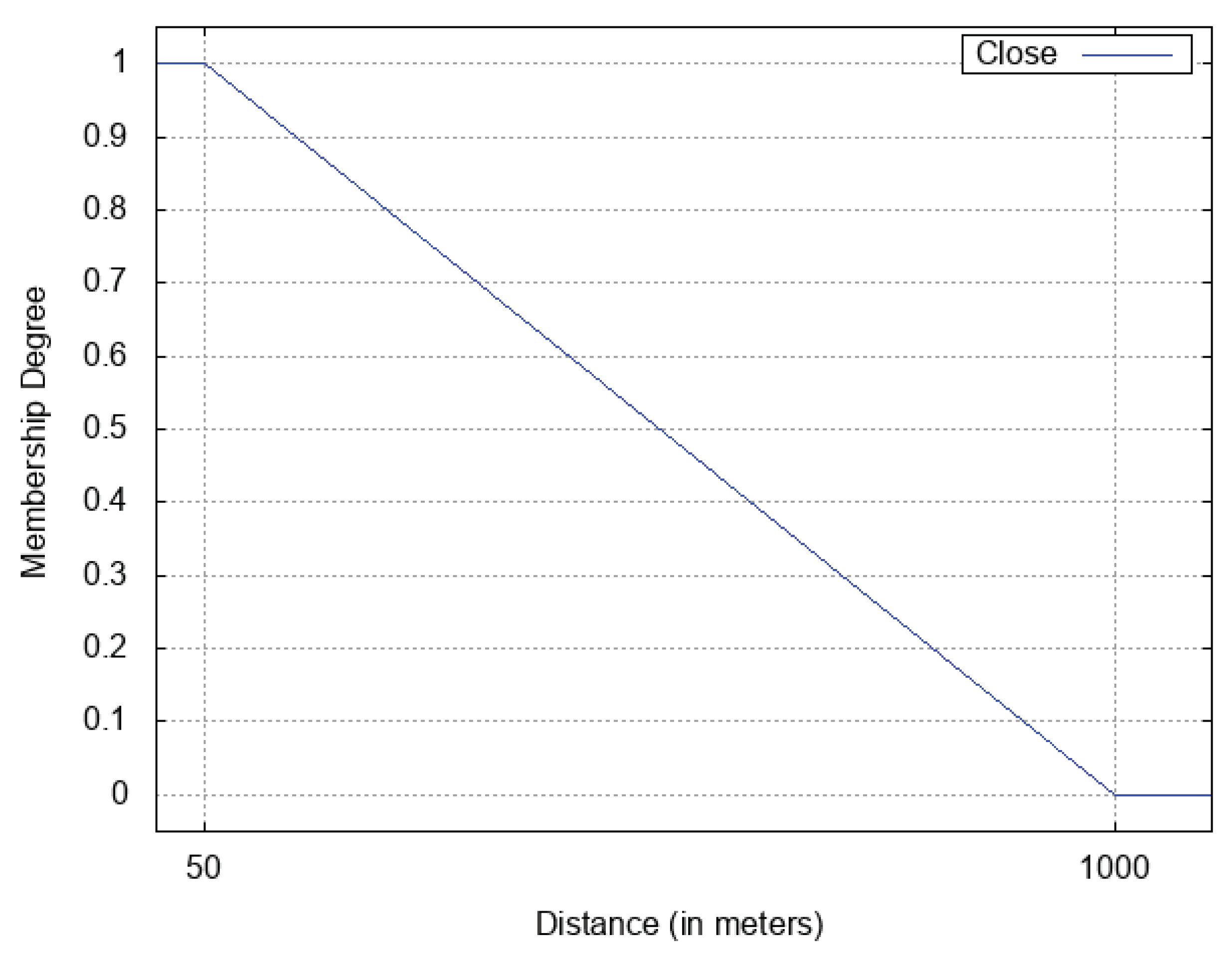
We considered five different values for the β g e o parameter (0.15; 0.30; 0.50; 0.70; 0.85) so as to evaluate the effect of the geographical contribution, by varying its weight from a very small weight to a very high weight. We also considered three different values for the α parameter (0.65; 0.75; 0.85), in order to evaluate the effect of increasing the threshold (the greater the threshold, the stronger the membership degree necessary to classify a pair as “Good”). As far as the C l o s e relation is concerned, we ran all the experiments with m i n d = 50 m and m a x d = 1000 m.
We evaluated recall, precision, and F1-score. Remember that recall represents the ratio between the number of descriptor pairs labeled as “Good” by the technique that were labeled with “Yes” by hand (the true positive pairs) and the total number of descriptor pairs labeled with “Yes” by hand (formally, r e c a l l = T P T P + F N , where T P stands for “true positive” and F N stands for “false negative”). Then, remember that precision represents the ratio between the number of descriptor pairs labeled as “Good” by the technique which were labeled with “Yes” by hand and the total number of descriptor pairs labeled as “Good” by the technique (formally, p r e c i s i o n = T P T P + F P , where F P stands for “false positive”). Finally, remember that F1-score (or F1) represents a combined/synthetic metric of recall and precision: it is defined as F1-score = r e c a l l × p r e c i s i o n r e c a l l + p r e c i s i o n × 2 .
Table 2 reports the results of our experiments performed on Manchester test set; Table 3 reports the results of our experiments performed on Genoa test set; Table 4 reports the results of our experiments performed on Stuttgart test set.
In order to easily conduct the sensitivity analysis, results in Table 2, Table 3 and Table 4 are plotted, respectively, in Figure 3, Figure 4 and 
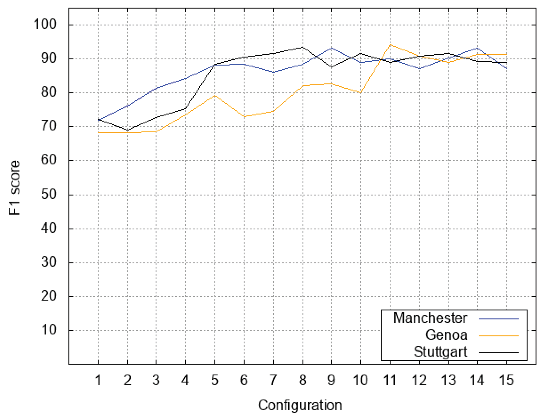
Figure 5. In particular, 
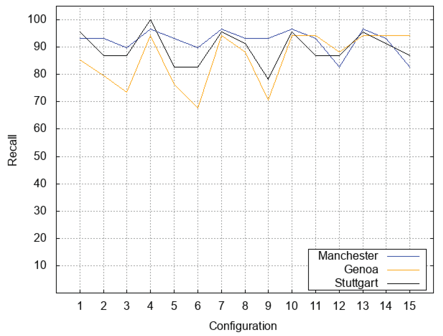
Figure 3 plots how recall varies depending on the variation of configuration settings; the blue line plots results obtained with the Manchester test set, the orange line plots how recall varies for the Genoa test set, and the black line plots how recall varies for the Stuttgart test set. We can notice that Genoa test set was quite sensitive to variations of the β g e o parameter; we observe that the orange line becomes stable for configurations C o n f 13 , C o n f 14 , and C o n f 15 . The other two test sets were more stable; nevertheless, all three lines reached a good stability for the last three configurations.
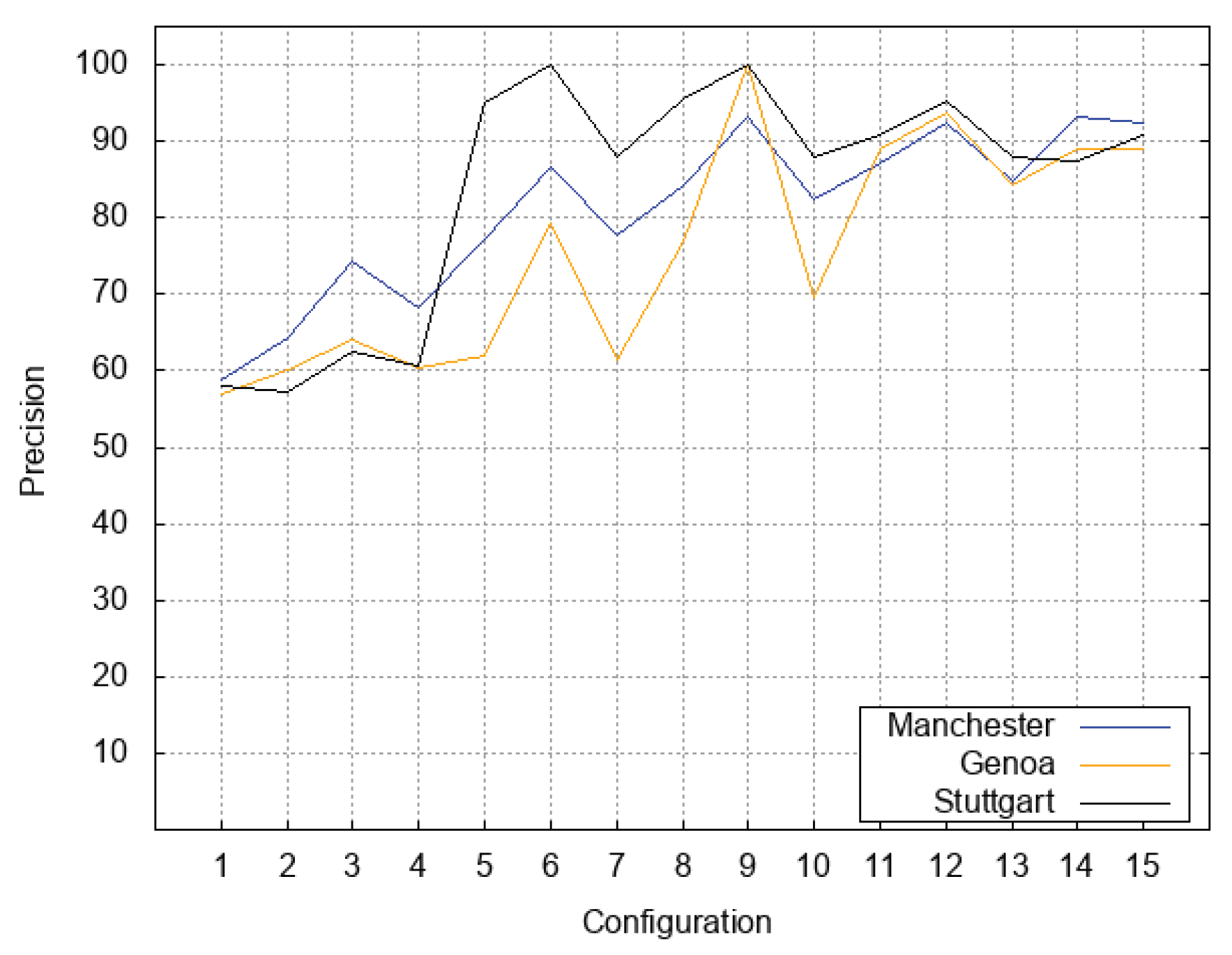
Figure 4 plots precision obtained for the three test sets for all the 15 configurations. Note how increasing values of the β g e o parameter strongly influence precision, which substantially increases. Even though for Genoa test set (orange line) we obtain the best precision with C o n f 9 and for Stuttgart test set (black line) we obtain the best precision also with C o n f 4 ; all three curves become stable for configurations C o n f 13 , C o n f 14 and C o n f 15 , confirming what emerged by analyzing plots for recall (Figure 3).
Figure 5 plots the behavior of F1-score, for the three test sets with all the 15 configurations. The F1-score is quite useful to analyze the behavior in an aggregated way. We can see that the three lines all converge to show stable and good results for configurations from C o n g 11 to C o n f 15 . This confirms that high values of the β g e o parameter obtained the best results, while changes in the α parameter usually got little effects for high values of the β g e o parameter.
After this analysis, it is possible to see that configuration C o n f 14 can be chosen as the reference configuration for our technique, because it obtained the best combination of recall, precision, and F1-score for the three test sets.
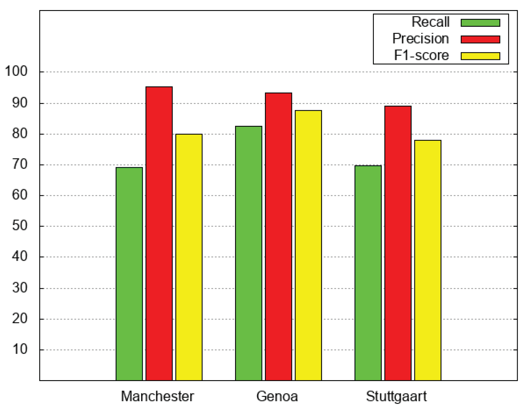
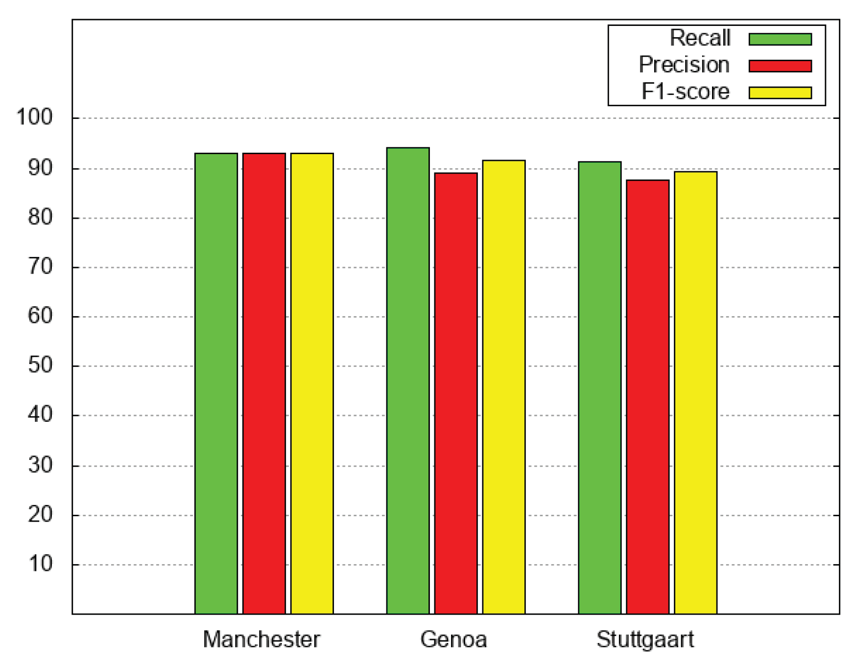
Table 5 reports, in the upper part, the results obtained by applying the M a t c h i n g P l a c e s V 1 relation (see Definition 6), that is the baseline definition of the M a t c h i n g P l a c e s relation; in the middle, the table reports the results obtained for the M a t c h i n g P l a c e s V 2 relation with C o n f 14 as reference configuration. Recall (from Section 5.2) that, as far as the C l o s e relation is concerned, we run experiments for the M a t c h i n g P l a c e s V 1 relation with settings m i n d = 100 m and m a x d = 2000 m, as in [9]; furthermore, the minimum threshold to defuzzify is α = 0.75 .
The table clearly shows that the novel formulation of the M a t c h i n g P l a c e s relation (denoted as M a t c h i n g P l a c e s V 2 ) always outperforms the baseline version (denoted as M a t c h i n g P l a c e s V 1 ) as far as recall and F1-score are concerned.
In particular, notice that we obtained 93 % for F1-score, recall and precision for the Manchester test set.
Figure 6 and Figure 7 depict the results reported in the upper and middle parts of Table 5. Specifically, green bars denote recall, red bars denote precision and yellow bars denote F1-score.
It is possible to notice that the baseline has good performance with Italian language, while it does not perform so well with English and German languages. This is due to the fact that the Manchester test set and Stuttgart test set have a significant number of missing fields. This confirms that the novel formulation of the M a t c h i n g P l a c e s relation is actually effective in dealing with such missing fields.

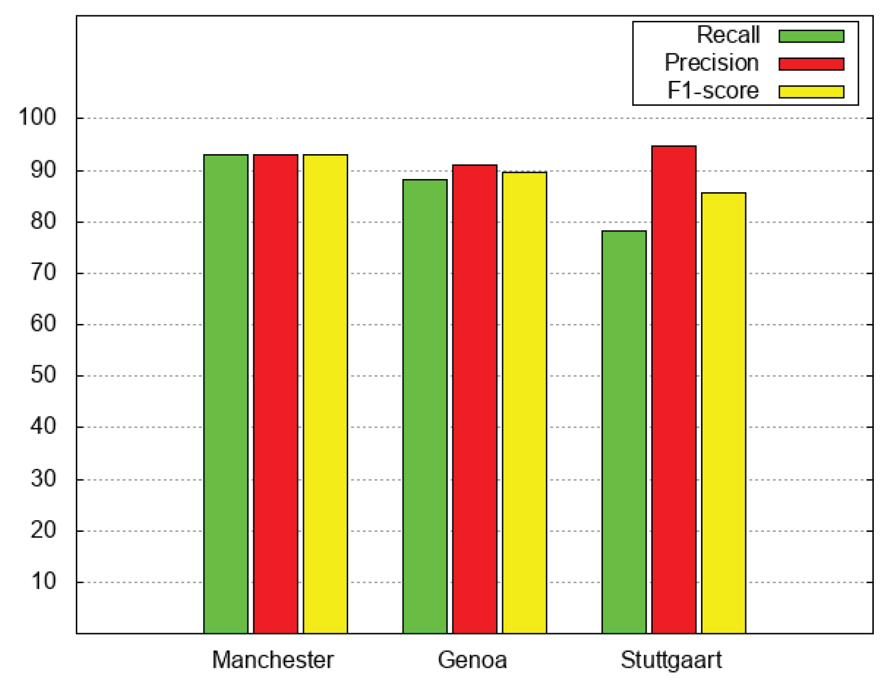
6.2. Comparison with Random-Forest Classifiers

We now compare our technique with the machine-learning technique known as “random forest”. It is a known supervised ensemble learning method for classification devised by Ho [29]. In a supervised learning method, there are two types of variables: many features that are the input independent variables; and one target that is the output dependent variable (individual classes into which the input variables maybe mapped). The name of the technique is motivated by the fact that, during the training phase, many classification trees are generated (i.e., a forest of classification trees). During the test phase, all the classification trees are exploited and the class assigned by the majority of them is taken.
We chose the random-forest technique because it was used by Santos et al. [1] to compare the performances of different string similarity metrics in the task known as toponym matching.
We performed experiments by adopting the Python library named ML provided within the sklearn module; specifically, we exploited the method named RandomForestClassifier. In particular, we configured its parameters as follows:
  • f e a t u r e s _ n u m b e r = 3 , out of 3 (instead of # f e a t u r e s );
  • t r e e s _ n u m b e r = 10 (default value);
  • s p l i t _ c r i t e r i o n = g i n i (default value).
Hereafter, we discuss the choices. We chose three out of three features (instead of # f e a t u r e s , where # f e a t u r e s is the total number of features in the data set) in order to compare it with our technique. These features are: the membership degree of the W i n k l e r relation evaluated on names; the membership degree of the W i n k l e r relation evaluated on addresses; the distance (in meters) between locations. Finally, for each tree of the random forest, the Gini impurity criterion serves to split the sample in each node.
For each training set, we generated three distinct classifiers. So, we have a random forest for Manchester training set, one for Genoa training set and one for Stuttgart training set. Recall that each training set contains 300 pairs of descriptors, while each test set contains 100 pairs of descriptors.
Table 5 compares performances shown by the random-forest technique (bottom part) with performances obtained by our technique (middle part of the table), with configuration Conf14, that is the configuration that provided the best average performance. Furthermore, Figure 8 compares recall (green bars), precision (red bars), and F1-score (yellow bar) obtained by applying the random-forest technique to the three test sets (denoted as Manchester, Genoa, and Stuttgart), as opposed to Figure 7, that compares performances obtained by the M a t c h i n g P l a c e s V 2 relation with configuration C o n f 14 .
We can notice that as far as recall and F1-score are concerned, our technique always outperformed (even slightly) the random-forest technique. In particular, while with the Manchester test set the results were the same, our technique behaveed better with Genoa test set and Stuttgart test set.
In contrast, the random forest technique behaved better in terms of precision with Genoa test set and Stuttgart test sets. This means that the classifier based on random forests retrieved fewer false positive pairs of descriptors. In any case, the higher recall shown by our technique significantly compensates the slightly lower precision of our technique, as shown by the F1-score.
Consequently, we can conclude that our technique is effective as much as random-forest classifiers, and sometimes it is slightly better. This confirms that our approach is good for performing the on-line aggregation of place descriptors coming from different social media, in that it does not require any preliminary training phase and behaves as random-forest classifiers that, in contrast, require a preliminary training phase.

7. Conclusions

In this paper, we addressed the problem of on-line aggregating information concerning public places and points of interest gathered and published by social media. The goal is to develop a tool able to provide users with a unique and aggregated view of all pieces of information concerning the same public place.
We proposed a fuzzy technique based on a binary fuzzy relation named M a t c h i n g P l a c e s : by relying on possibility theory; the proposed relation allows us to make a hypothesis about the fact that two place descriptors actually describe the same place, without prior knowledge. In order to validate the approach, we tested it on three real-life data sets, concerning Manchester (UK), Genoa (Italy), and Stuttgart (Germany), downloaded from Google Places and Facebook. We compared the new technique with the preliminary version proposed in [9], that we used as baseline: experiments show that the new version significantly outperforms the baseline, meaning that it deals with anomalies better than the baseline. Furthermore, we compared it to the well known off-line classification technique called random forest: we could see that the two techniques obtained comparable results; however, to build a random-forest classifier, a preliminary download and a training phase preceded by hand-made labeling of data were necessary; our technique can be directly applied on-line, when querying social-media APIs.
The reader could wish to understand if the proposed approach, based on the adoption of fuzzy relations, could be applied to different application contexts, always related to social media but not concerning public places. If this question is intended as “is it possible to apply the same complex MatchingPlaces relation as it is to conflate lists of triples (name, address, location) not describing public places?”, the answer is “yes, it can be applied as it is”. In this case, we would obtain two advantages: (i) no preliminary training phase on data would be necessary, because our relation does not require training; (ii) the reason why two items are aggregated is clearly explained by the definition of the MatchingPlaces relation. In contrast, if the problem to address could not be formulated as we said, we could expect that other complex fuzzy relations should be defined, possibly reusing basic fuzzy relations concerned with string similarity or closeness; in fact, the fuzzy approach is general and can be applied when imprecision and uncertainty must be addressed, but relations must be specifically designed for the specific problem.
In the future, we will further refine our technique, by designing new fuzzy relations that exploit different fuzzy aggregation operators; moreover, we will compare our method with other machine-learning methods. Finally, we think that the M a t c h i n g P l a c e s relation should be parameterized with respect to the size of the geographical area of interest and number of inhabitants in cities, in order to tailor the aggregation technique to the specific context. Notice that this is a different kind of prior knowledge, if compared with the knowledge provided by labeling training sets for off-line classifiers; in fact, this knowledge describes the geo-political context in which public places are, and can l be acquired on-line, by querying specific web services.

Author Contributions

Conceptualization, G.P.; methodology, G.P.; software, M.T.; validation, G.P. and M.T.; investigation, G.P. and M.T.; data curation, M.T.; writing—original draft preparation, G.P. and M.T.; writing—review and editing, G.P.; supervision, G.P.

Funding

This research was funded by the Dept. of Management, Information and Product Engineering of the University of Bergamo, that enrolled Maurizio Toccu from May 1, 2018 to April 30, 2019 as research assistant.

Conflicts of Interest

The authors declare no conflict of interest.

References

  1. Santos, R.; Murrieta-Flores, P.; Martins, B. Learning to combine multiple string similarity metrics for effective toponym matching. Int. J. Digit. Earth 2018, 11, 913–938. [Google Scholar] [CrossRef]
  2. Rui, S.; Patricia, M.F.; Pavel, C.; Bruno, M. Toponym matching through deep neural networks. Int. J. Geogr. Inf. 2018, 32, 324–348. [Google Scholar]
  3. McKenzie, G.; Zheng, L.; Yingjie, H.; Myeong, L. Identifying Urban Neighborhood Names through User-Contributed Online Property Listings. ISPRS Int. J. Geo-Inf. 2018, 7, 388. [Google Scholar] [CrossRef] [Green Version]
  4. Kilinc, D. An Accurate Toponym-Matching Measure Based On Approximate String Matching. J. Inf. Sci. 2016, 42, 138–149. [Google Scholar] [CrossRef]
  5. Hastings, J. Automated conflation of digital gazetteer data. Int. J. Geogr. Inf. Sci. 2008, 22, 1109–1127. [Google Scholar] [CrossRef]
  6. Jung, O.K.; Kiyun, Y.; Joon, H.; Won Hee, L. A New Method for Matching Objects in Two Different Geospatial Datasets Based On the Geographic Context. Comput. Geosci. 2010, 36, 1115–1122. [Google Scholar]
  7. Zadeh, L.A. Fuzzy sets as a basis for a theory of possibility. Fuzzy Sets Syst. 1978, 1, 3–28. [Google Scholar] [CrossRef]
  8. Bunke, H.; Fàbregas, X.; Kandel, A. Rule-based fuzzy object similarity. Mathw. Soft Comput. 2001, 8, 113–128. [Google Scholar]
  9. Toccu, M.; Psaila, G.; Altomare, D. On-line Aggregation of POIs from Google and Facebook. In Proceedings of the SAC 2019 ACM Symposium on Applied Computing, Limassol, Cyprus, 8–12 April 2019; pp. 1081–1089. [Google Scholar]
  10. Bentley, F.; Cramer, H.; Müller, J. Beyond the bar: The places where location-based services are used in the city. Pers. Ubiquitous Comput. 2015, 19, 217–223. [Google Scholar] [CrossRef]
  11. McKenzie, G.; Janowicz, K.; Adams, B. A weighted multi-attribute method for matching user-generated points of interest. Cartogr. Geogr. Inf. Sci. 2014, 41, 125–137. [Google Scholar] [CrossRef]
  12. Li, Y.; Peiyuan, Q.; Xiliang, L.; Feng, L.; Bo, W. A Holistic Approach to Aligning Geospatial Data with Multidimensional Similarity Measuring. Int. J. Digit. Earth 2018, 11, 845–862. [Google Scholar]
  13. Li, L.; Xing, X.; Xia, H.; Huang, X. Entropy-Weighted Instance Matching Between Different Sourcing Points of Interest. Entropy 2016, 18, 45. [Google Scholar] [CrossRef] [Green Version]
  14. Bordogna, G.; Pagani, M.; Pasi, G.; Psaila, G. Flexible location-based spatial queries. In Theoretical Advances and Applications of Fuzzy Logic and Soft Computing; Springer: Berlin, Germany, 2007; pp. 36–45. [Google Scholar]
  15. Bordogna, G.; Pagani, M.; Pasi, G.; Psaila, G. Evaluating uncertain location-based spatial queries. In Proceedings of the 2008 ACM symposium on Applied computing, Ceara, Brazil, 16–20 March 2008; pp. 1095–1100. [Google Scholar]
  16. Bordogna, G.; Pagani, M.; Pasi, G.; Psaila, G. Managing uncertainty in location-based queries. Fuzzy Sets Syst. 2009, 160, 2241–2252. [Google Scholar] [CrossRef]
  17. Bordogna, G.; Psaila, G. Extending SQL with customizable soft selection conditions. In Proceedings of the 2005 ACM symposium on Applied computing, Santa Fe, NM, USA, 13–17 March 2005; pp. 1107–1111. [Google Scholar]
  18. Bordogna, G.; Psaila, G. Soft Aggregation in Flexible Databases Querying based on the Vector p-norm. Int. J. Uncertain. Fuzziness Knowl. Based Syst. 2009, 17, 25–40. [Google Scholar] [CrossRef]
  19. Bordogna, G.; Campi, A.; Psaila, G.; Ronchi, S. An interaction framework for mobile web search. In Proceedings of the 6th International Conference on Advances in Mobile Computing and Multimedia, Linz, Austria, 24–26 November 2008; pp. 183–191. [Google Scholar]
  20. Bordogna, G.; Campi, A.; Psaila, G.; Ronchi, S. A language for manipulating clustered web documents results. In Proceedings of the 17th ACM conference on Information and knowledge management, Napa Valley, CA, USA, 26–30 October 2008; pp. 23–32. [Google Scholar]
  21. Bordogna, G.; Campi, A.; Psaila, G.; Ronchi, S. Query disambiguation based on novelty and similarity user’s feedback. In Proceedings of the International Conference on Flexible Query Answering Systems, Roskilde, Denmark, 26–28 October 2009; Springer: Berlin, Germany, 2009; pp. 179–190. [Google Scholar]
  22. Zadeh, L. Fuzzy Sets. Inf. Control 1965, 8, 338–353. [Google Scholar] [CrossRef] [Green Version]
  23. Zadeh, L.A. The concept of a linguistic variable and its application to approximate reasoning—I. Inf. Sci. 1975, 8, 199–249. [Google Scholar] [CrossRef]
  24. Zadeh, L.A. The concept of a linguistic variable and its application to approximate reasoning—II. Inf. Sci. 1975, 8, 301–357. [Google Scholar] [CrossRef]
  25. Xu, Z. Intuitionistic fuzzy aggregation operators. IEEE Trans. Fuzzy Syst. 2007, 15, 1179–1187. [Google Scholar]
  26. Jaro, M.A. UNIMATCH, A Record Linkage System: Users Manual; Bureau of the Census: Suitland, MD, USA, 1980.
  27. Jaro, M.A. Advances in record-linkage methodology as applied to matching the 1985 census of Tampa, Florida. J. Am. Stat. Assoc. 1989, 84, 414–420. [Google Scholar] [CrossRef]
  28. Winkler, W.E. String Comparator Metrics and Enhanced Decision Rules in the Fellegi-Sunter Model of Record Linkage. In Proceedings of the Section on Survey Research Methods, American Statistical Association, Anaheim, CA, USA, 6–9 August 1995; pp. 354–359. [Google Scholar]
  29. Ho, T.K. Random Decision Forests. In Proceedings of the 3rd International Conference on Document Analysis and Recognition, Montreal, QC, Canada, 14–16 August 1995; pp. 278–282. [Google Scholar]
Figure 1. On-line Aggregation Scenario.
Information 10 00388 g001
Figure 2. Membership function for the Close relation.
Information 10 00388 g002
Figure 3. Sensitivity analysis of recall for relation M a t c h i n g P l a v e s V 2 .
Information 10 00388 g003
Figure 4. Sensitivity analysis of precision for relation M a t c h i n g P l a v e s V 2 .
Information 10 00388 g004
Figure 5. Sensitivity Analysis of F1-score for relation M a t c h i n g P l a v e s V 2 .
Information 10 00388 g005
Figure 6. Performance of M a t c h i n g P l a c e s V 1 relation.
Information 10 00388 g006
Figure 7. Performance of M a t c h i n g P l a c e s V 2 relation with setting C o n f 14 .
Information 10 00388 g007
Figure 8. Performance of random forest machine-learning technique.
Information 10 00388 g008
Table 1. Configurations for parameters β g e o (contribution of geographical information) and α (threshold to de-fuzzify).
Conf β geo α
C o n f 1 0.65
C o n f 2 0.150.75
C o n f 3 0.85
C o n f 4 0.65
C o n f 5 0.300.75
C o n f 6 0.85
C o n f 7 0.65
C o n f 8 0.500.75
C o n f 9 0.85
C o n f 10 0.65
C o n f 11 0.700.75
C o n f 12 0.85
C o n f 13 0.65
C o n f 14 0.850.75
C o n f 15 0.85
Table 2. Sensitivity analysis shown by the M a t c h i n g P l a c e s V 2 relation on Manchester test set.
Conf β geo α RecallPrecisionF1-Score
C o n f 1 0.6593.10%58.70%72.00%
C o n f 2 0.150.7593.10%64.29%76.06%
C o n f 3 0.8589.66%74.29%81.25%
C o n f 4 0.6593.10%77.14%84.38%
C o n f 5 0.300.7589.66%86.67%88.14%
C o n f 6 0.8593.10%84.38%88.52%
C o n f 7 0.6596.55%77.78%86.15%
C o n f 8 0.500.7593.10%84.38%88.52%
C o n f 9 0.8593.10%93.10%93.10%
C o n f 10 0.6596.55%82.35%88.89%
C o n f 11 0.700.7593.10%87.10%90.00%
C o n f 12 0.8582.76%92.31%87.27%
C o n f 13 0.6596.55%84.85%90.32%
C o n f 14 0.850.7593.10%93.10%93.10%
C o n f 15 0.8582.76%92.31%87.27%
Table 3. Sensitivity analysis shown by the M a t c h i n g P l a c e s V 2 relation on Genoa test set.
Conf β geo α RecallPrecisionF1-Score
C o n f 1 0.6585.29%56.86%68.24%
C o n f 2 0.150.7579.41%60.00%68.35%
C o n f 3 0.8573.53%64.10%68.49%
C o n f 4 0.6594.12%60.38%73.56%
C o n f 5 0.300.7576.47%61.90%79.31%
C o n f 6 0.8567.65%68.42%73.02%
C o n f 7 0.6594.12%61.54%74.42%
C o n f 8 0.500.7588.24%76.92%82.19%
C o n f 9 0.8570.59%100.00%82.76%
C o n f 10 0.6594.12%69.57%80.00%
C o n f 11 0.700.7594.12%88.89%94.13%
C o n f 12 0.8588.24%93.75%90.91%
C o n f 13 0.6594.12%84.21%88.89%
C o n f 14 0.850.7594.12%88.89%91.43%
C o n f 5 0.8594.12%88.89%91.43%
Table 4. Sensitivity analysis shown by the M a t c h i n g P l a c e s V 2 relation on Stuttgart test set.
Conf β geo α RecallPrecisionF1-Score
C o n f 1 0.6595.65%57.89%72.13%
C o n f 2 0.150.7586.96%57.14%68.97%
C o n f 3 0.8586.96%62.50%72.73%
C o n f 4 0.65100.00%60.53%75.41%
C o n f 5 0.300.7582.61%95.00%88.37%
C o n f 6 0.8582.61%100.00%90.48%
C o n f 7 0.6595.65%88.00%91.67%
C o n f 8 0.500.7591.30%95.45%93.33%
C o n f 9 0.8578.26%100.00%87.80%
C o n f 10 0.6595.65%88.00%91.67%
C o n f 11 0.700.7586.96%90.91%88.89%
C o n f 12 0.8586.96%95.24%90.91%
C o n f 13 0.6595.65%88.00%91.67%
C o n f 14 0.850.7591.30%87.50%89.36%
C o n f 15 0.8586.96%90.91%88.89%
Table 5. Evaluation of recall, precision and F1-score for C o n f 14 ( β = 0.85 , threshold = 0.75).
MatchingPlaces V 1 RecallPrecisionF1-Score
Manchester (UK)68.97%95.24%80.00%
Genoa (Italy)82.35%93.33%87.50%
Stuttgart (Germany)69.57%88.89%78.05%
MatchingPlaces V 2 RecallPrecisionF1-Score
Manchester (UK)93.10%93.10%93.10%
Genoa (Italy)94.12%88.89%91.43%
Stuttgart (Germany)91.30%87.50%89.36%
Randomforest RecallPrecisionF1-Score
Manchester (UK)93.10%93.10%93.10%
Genoa (Italy)88.24%90.91%89.55%
Stuttgart (Germany)78.26%94.74%85.71%

