Using a Long Short-Term Memory Recurrent Neural Network (LSTM-RNN) to Classify Network Attacks

Abstract

An intrusion detection system (IDS) identifies whether the network traffic behavior is normal or abnormal or identifies the attack types. Recently, deep learning has emerged as a successful approach in IDSs, having a high accuracy rate with its distinctive learning mechanism. In this research, we developed a new method for intrusion detection to classify the NSL-KDD dataset by combining a genetic algorithm (GA) for optimal feature selection and long short-term memory (LSTM) with a recurrent neural network (RNN). We found that using LSTM-RNN classifiers with the optimal feature set improves intrusion detection. The performance of the IDS was analyzed by calculating the accuracy, recall, precision, f-score, and confusion matrix. The NSL-KDD dataset was used to analyze the performances of the classifiers. An LSTM-RNN was used to classify the NSL-KDD datasets into binary (normal and abnormal) and multi-class (Normal, DoS, Probing, U2R, and R2L) sets. The results indicate that applying the GA increases the classification accuracy of LSTM-RNN in both binary and multi-class classification. The results of the LSTM-RNN classifier were also compared with the results using a support vector machine (SVM) and random forest (RF). For multi-class classification, the classification accuracy of LSTM-RNN with the GA model is much higher than SVM and RF. For binary classification, the classification accuracy of LSTM-RNN is similar to that of RF and higher than that of SVM.

1. Introduction

With the rapid growth of networks in accessing valuable information, network-based services are growing faster than ever before. This situation has raised the number of cyber offense cases. A network intrusion detection system (NIDS) is a tool that detects malicious activities in a system that violate security and privacy. Any malicious activity is typically reported to an administrator or collected centrally. A security information and event management (SIEM) system collects and combines information about malicious activities from multiple sources and distinguishes malicious activity from false alarms. Denning (1987) implemented an IDS for the first time [1], and since then, research on IDS has developed to provide better solutions that may protect network systems from various types of network attacks.

Organizations are using NIDSs to protect their systems from attacks that come with network connectivity. NIDSs are classified into two categories: (1) signature-based NIDSs and (2) anomaly-based NIDSs. A signature-based NIDS filters the signatures of the attack patterns. The analysis is static and is limited to the detection of only known attack patterns. Signature-based NIDSs give high accuracy and low false-alarm rates for detecting known attacks, but they have poor performance when detecting unknown or new attacks. In an anomaly-based NIDS, heuristic methods are used for detecting unknown attacks. When a deviation is observed in normal traffic, the anomaly-based NIDS classifies the traffic as an intrusion; this tends to produce a high false-positive rate. Despite this, anomaly-based NIDSs have wide acceptance in research because of the theoretical potential in the identification of novel attacks.

Machine learning approaches such as support vector machine (SVM) and decision tree (DT) were used on the 1998 DARPA intrusion detection dataset [2]. In research reported in [3] and [4], the authors used a decision tree-based model on the NSL-KDD datasets. Random forests (RF) [5], k-means [6], naïve Bayes (NB) [7], multilayer perceptrons [8], and artificial neural networks (ANN) [9] have also been used in developing NIDSs. Deep learning approaches have been successfully used in voice, image, and face detection [10,11].

Commonly used deep learning-based approaches include the deep neural network (DNN) [12,13], the recurrent neural network (RNN) [14,15], the convolutional neural network (CNN) [16], the deep belief network (DBN) [17], and long short-term memory (LSTM) [18,19,20,21]. In [22], a deep learning-based technique called self-taught learning (STL) was applied to the NSL-KDD dataset to develop an effective NIDS. Using the LSTM-RNN method gave a high detection rate on the KDD Cup’99 datasets [18]. Research showed that LSTM-RNN performed better than SVM, KNN (K-nearest neighbors), Bayes, probabilistic neural networks (PNNs), and some other neural network models.

In developing a flexible and effective NIDS for unknown attacks, it is difficult to select a proper feature set from the network traffic dataset. The features of one class of attack may not be applicable to another class of attack because of the changing nature of attack scenarios. In [19], a researcher applied post-pruned DTs and backward elimination for feature selection. They applied the J4.8 decision tree algorithm which moves the nodes up towards the root of the tree and discards other nodes on the way. After building the first tree from the training set with all features, those features were removed from the dataset which were not part of the tree.

To extract relevant features from the training set, feature selection is performed to eliminate the insignificant training features, as emphasized in [23]. In that research, the authors showed that a chosen set of features may highly affect the accuracy of a classifier. Feature selection can be done through three approaches, namely, as a filter, as a wrapper, or as in an embedded way. The filter approach selects the most significant features regardless of the model used. Its main advantages are low execution time and its ability to solve the over-fitting problem. The wrapper approach combines related features into a subset. Its main benefit is its ability to consider the interaction between features although it has a high execution time and is prone to over-fitting. Finally, the embedded approach investigates the interaction between the features in a deeper manner than the wrapper, so it can produce an optimal subset of significant features, although it has a high execution time also.

In this research, we developed a new NIDS by combining GA for optimal feature selection and LSTM-RNN. The NIDS was used to classify the NSL-KDD dataset, a benchmark dataset for NIDSs. Both binary and multi-class/5-category classification was done in this experiment. The hyper-parameter set may affect the performance of an LSTM-RNN classifier. Through several experiments, an optimal hyper-parameter set, which includes learning rate, batch size, epoch, optimizer, activation function, and loss function, was established for the LSTM-RNN model dataset.

Results show that applying the GA gave a much higher accuracy than using the original feature set. Furthermore, results show that LSTM-RNN with the GA classifier can learn all attack classes in the training data. The classifier could detect a large number of all attacks accurately from the test data. Therefore, LSTM-RNN with the GA can decrease the amount of misclassification over what results when using the entire feature set. Performance metrics such as training accuracy and testing accuracy, precision, recall, f-score, true positive rate (TPR), false-positive rate (FPR) and confusion matrix were calculated in this research. A comparison of the performance of LSTM-RNN (with the GA) with SVM and random forest was also conducted. The results show that LSTM-RNN performs very well in both binary and multiclass classification. The accuracy is about 93.88% for multi-class classification and about 99.91% for binary classification. LSTM-RNN also provided a high TPR and a low FPR.

The rest of the paper is organized as follows. Section 2 provides the background on deep learning, long short-term memory (LSTM) networks, recurrent neural networks (RNNs), and genetic algorithms (GAs). It also describes the NSL-KDD dataset, which is used in the research. Section 3 discusses the existing research on LSTM and RNN in NIDS, which is related to this research. Section 4 presents the methodology of the LSTM-RNN with the GA model in detail. Section 5 presents the results of various experiments as well as a performance comparison of several classifiers. In Section 6, we discuss the results of our experiments. Finally, we provide conclusions and future work in Section 7.

2. Background

2.1. Deep Learning Architecture

Deep learning is one of the machine learning methods that implements artificial neural networks. A deep learning network is a multi-layer neural network. Deep learning networks include deep neural networks (DNN), convolutional neural networks (CNN), recurrent neural networks (RNN), deep belief networks (DBN), and others. In this section, we will describe the architecture of RNN and long short-term memory (LSTM).

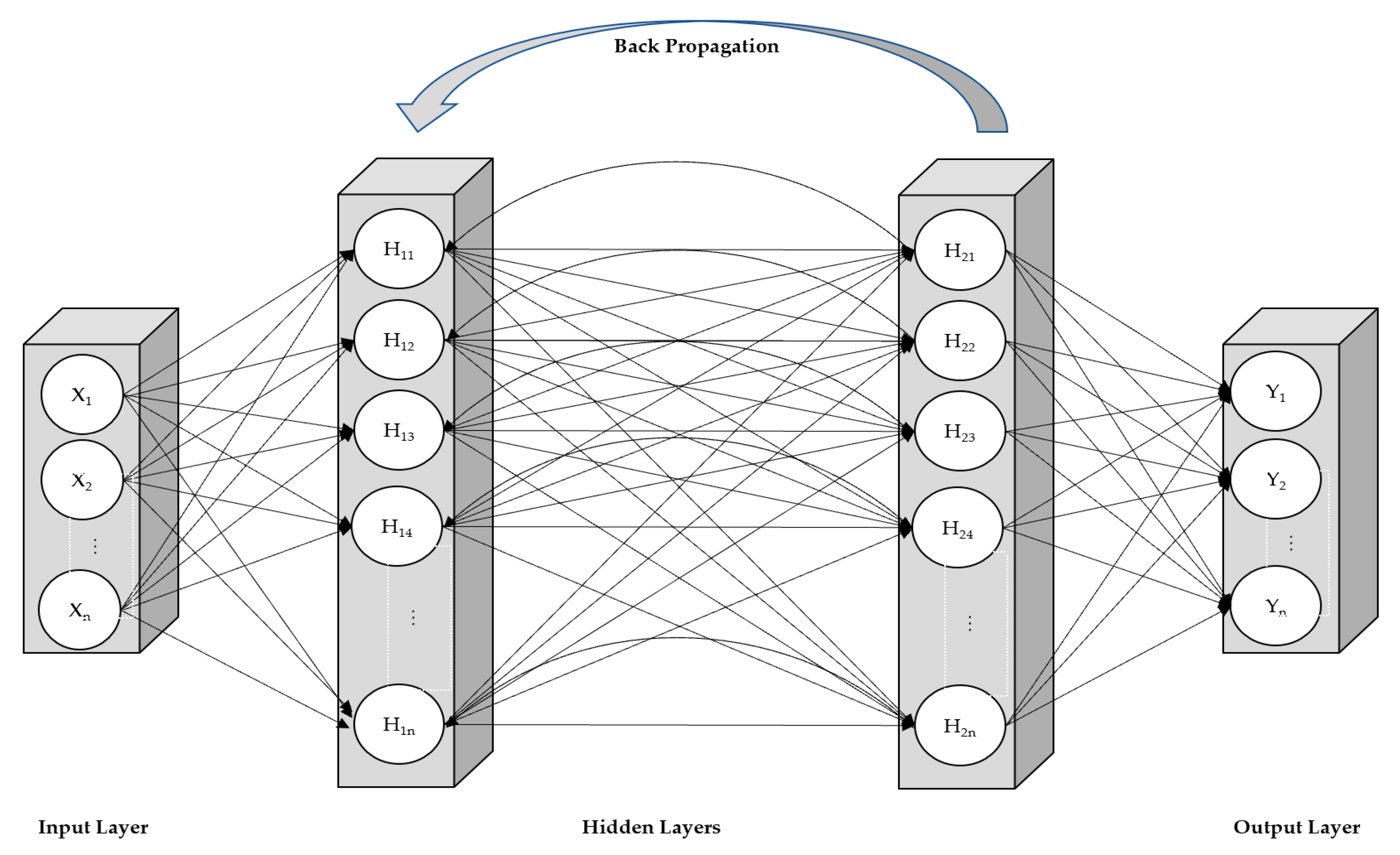
2.1.1. Recurrent Neural Network (RNN)

RNN is a type of artificial neural network (ANN), wherein the connection between the nodes resembles the neurons of a human brain. Neural network connections can transmit signals to other neurons/nodes [24] like synapses in a biological brain. The artificial neuron then processes the received signal and transmits it to the other connected neurons/nodes. Neurons and connections typically have weights to adjust the learning process. The weight can vary to adjust the strength of the signal as the signal travels from the input layers to the output layers. An ANN contains hidden layers between the input and output layers. RNN should have at least three hidden layers. The basic architecture of RNNs includes input units, output units, and hidden units, with the hidden units performing all the calculations by weight adjustment to produce the outputs [18,25,26]. The RNN model has a one-way flow of information from the input units to the hidden units and a directional loop that compares the error of this hidden layer to that of the previous hidden layer, and adjusts the weights between the hidden layers. Figure 1 represents a simple RNN architecture with two hidden layers.

An RNN is an extension of traditional feed-forward neural networks (FFNNs). In FFNNs, the information moves in only the forward direction; i.e., from the input nodes, through the hidden nodes, to the output nodes; there are no cycles or loops in the network. Hidden layers are optional in traditional FFNNs. We assume an input vector sequence, a hidden vector sequence, and an output vector sequence denoted by X, H, and Y, respectively. An input vector sequence is given as X = ($x_1$, $x_2$, …, $x_T$). A traditional RNN calculates the hidden vector sequence H = ($h_1$, $h_2$, …, $h_T$) and output vector sequence Y = ($y_1$, $y_2$, …, $y_T$) with t = 1 to T as follows:

$$h_t=\sigma \left(W_{xh}{x}_t+W_{hh}{h}_{t-1}+b_h\right)$$

(1)

$$y_t=W_{hy}{h}_t+b_y$$

(2)

where function σ is a nonlinearity activation function, W is a weight matrix, and b is a bias term. In Equation (1), h_t is the hidden layer output at t-time steps, and h_t−1 denotes the previous hidden layer’s output.

RNN uses gradient-based methods to learn time sequences: back-propagation through time (BPTT) or real-time recurrent learning (RTRL) [27]. In BPTT, the network is unfolded into a multilayer FFNN in which each time a sequence is processed to construct the FFNN; firstly the training data is used to train the model and then the output error gradient is saved for each time step. BPTT uses the standard backpropagation algorithm to train each FFNN, and it updates the weights using the sum of the gradients obtained for weights in all layers of the network.

RTRL is an online learning algorithm, where the error gradient is computed, and weights are updated for each time step in a forward propagation manner. It computes the gradients of the internal and output nodes with respect to all the weights of the network.

Standard RNNs are not able to establish more than 5–10 time steps. A vanishing gradient problem may arise in RNN when gradient-based learning methods are used for updating the weights. Weights receive an updated proportion of the partial derivative of the error function in each training iteration. In some cases, the gradient will be very small. These error signals may either blow-up or vanish, which prevents the weight from changing value. These vanishing error signals may cause the weights to fluctuate. With a vanishing error, learning takes an unacceptable amount of time or does not work at all. In [25], a detailed theoretical analysis and solution of that problem with long-term dependencies is presented.

RNNs can be used for supervised classification learning [14,15]. RNNs are difficult to train because of vanishing and exploding gradients. The problems of vanishing and exploding gradients arise due to improperly assigned weights (assigned to either very high or very low value). Thus, an LSTM with forget gates is often combined with an RNN to overcome these training issues [26,27]. However, RNNs are a good choice for solving time series sequence prediction problems. In [18,19,20], researchers showed that some implementations of LSTM-RNN provide notable performance in intrusion detection. In [21], Staudemeyer et al. used LSTM-RNN on the KDD Cup’99 datasets and showed that LSTM-RNN could learn all attack classes hidden in the training data. They also learned from their experiment that the receiver operating characteristics (ROC) curve and the AUC (area under the ROC curve) are well suited for selecting high performing networks. The ROC curve is the probability curve plotting the TPR against the FPR, where TPR is on the y-axis and FPR is on the x-axis. A ROC curve shows the performance of a classification model at all classification thresholds. AUC value measures the entire two-dimensional area under the ROC curve. AUC values range from 0 to 1. AUC = 0.0 means the prediction of the model is 100% wrong and AUC = 1.0 means the prediction is 100% correct.

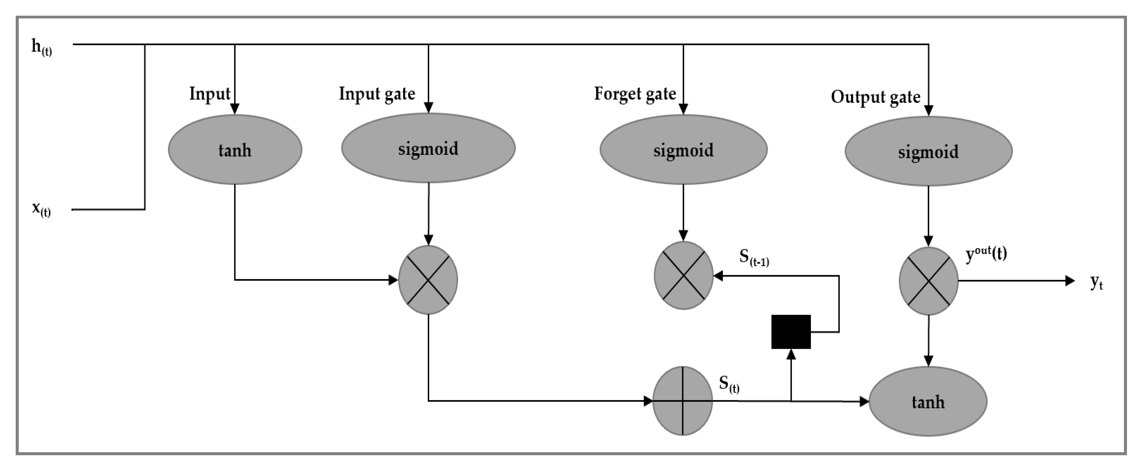
2.1.2. Long Short-Term Memory

LSTM can mitigate the problem of vanishing error [19,21,23]. LSTM can learn how to bridge more than 1000 discrete time steps [23]. LSTM networks replace all units in the hidden layer with memory blocks. Each memory block has at least one memory cell. Figure 2 demonstrates one cell in a basic LSTM network.

The memory cells activate with the regulating gates. These gates control the incoming and outgoing information flow. A forget-gate is placed between an input gate and an output gate. Forget gates can reset the state of the linear unit if the stored information is no longer needed. These gates are simple sigmoid threshold units. These activation functions range from 0 to 1.

The output $y^{c_j}\left(t\right)$ of an LSTM memory cell show in Figure 2 is computed as:

$$y^{c_j}\left(t\right)=y^{ou{t}_j}\left(t\right)h\left(s_{c_j}\left(t\right)\right)$$

where $y^{ou{t}_j}$ is the output gate activation, $s_{c_j}$ is the internal state of the output gate, and h is the hidden layer output.

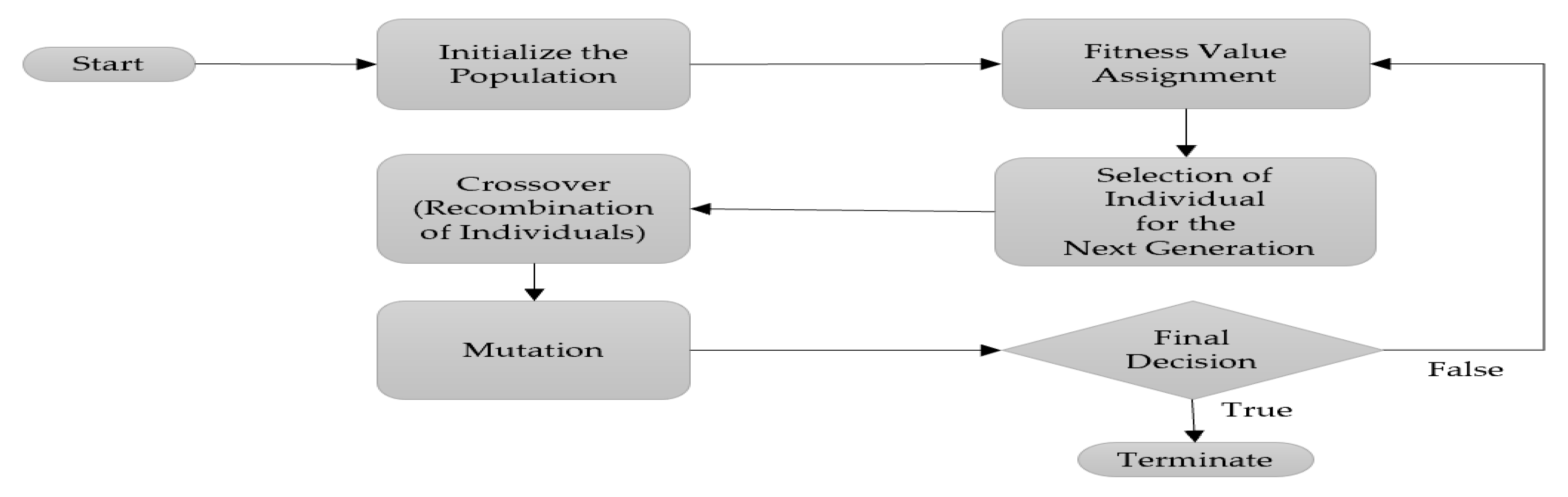
2.1.3. Genetic Algorithm (GA)

GAs are inspired by the concept of Darwin’s theory of evolution and execute evolutionary biology techniques, such as selection, mutation, recombination, and inheritance to solve a given problem. GA is a heuristic search method used for finding optimal solutions.

A GA [28] generates a pool of possible solutions for a given problem. It then creates a group of features/individuals randomly from the given problem. The individuals are then evaluated with evaluation functions provided by the programmer. These evaluation functions include some recombination and mutations, just as in natural genetics. Each of the solutions is assigned a fitness value, and the filtered individuals give a higher chance to fit into the model, thereby providing a list of good solutions rather than just one. GAs perform well in a large dataset where there are various features.

GAs provide various advantages in machine learning applications. They are used mostly in feature selection when many features need to be considered to predict a class in a classification problem. GAs can manage a dataset with many features, and they do not need any specific knowledge about the problem. A GA randomly generates solutions by recombination and mutation of the given features. Though this requires a lot of computation for building a predictive model, it can select the best subset of the features. As a result, using the GA solution, the NIDS model needs less execution time than when using the complete feature sets.

In this research, an NSL-KDD dataset is used which contains 125,973 records for training and 22,544 records for testing. Since a GA performs well on a large dataset, we applied GAs in this research to find the features that give near-optimal solutions. This not only minimized the training and testing time but also gave a high detection rate, a high true positive rate, and a low false alarm rate. A high positive rate and low false alarm rate indicates an ideal NIDS system. The outcomes of using GAs are presented in Section 5.

2.2. NSL-KDD Dataset

NSL-KDD is a refined version of the KDDCup’99 datasets. It removes all redundant records in the KDD Cup’99 so that unbiased classification results can be derived. By eliminating the duplicated data, a better detection rate can be achieved. The NSL-KDD dataset [29] contains KDDTrain+, which is a full training dataset including attack-type labels and difficulty levels in CSV format, and KDDTest+, which is a full testing dataset including attack-type labels and difficulty levels in CSV format. In the experiment in [29], the authors randomly created three subsets of the KDD training set with fifty thousand records. They employed 21 learning machines that had been formerly trained using the created training sets to label the records of the entire training and testing sets. This experiment provided 21 predicted labels for each record. The difficulty level of the NSL-KDD dataset denotes the number of successful prediction values obtained from each of the 21 learning machines. Successful prediction value conveys the number of learning machines that predicted the correct label. The highest difficulty level was 21 for any record in the dataset.

Table 1. Categories of attacks [30].

Major Categories	Subcategories
Denial of Service (DoS)	ping of Death, LAND, neptune, backscatter, smurf, teardrop
User to Root (U2R)	buffer Overflow, loadmodule, perl, rootkit
Remote to Local (R2L)	ftp-write, password guessing, imap, multi-hop, phf, spy, warezclient, warezmaster
Probing	ipsweeping, nmap, portsweeping, satan

and

Table 2. Total instances by attack type in the NSL-KDD dataset [31].

Attack	Total Instances in NSL-KDD Dataset	Attack Category
Back	956	DoS
Land	18
Neptune	41,214
Pod	201
Smurf	2646
Teardrop	892
Satan	3633
Ipsweep	3599	Probe
Nmap	1493
Portsweep	2931
Normal	67,343	Normal
guess-passwd	53	R2L
ftp-write	8
Imap	11
Phf	4
Multihop	7
Warezmaster	20
Warezclient	1020
Spy	2
buffer-overflow	30	U2R
Loadmodule	9
Perl	3
Rootkit	2931

characterize the NSL-KDD dataset.

The distribution of normal and attack records available in the NSL-KDD dataset is shown in

Table 3. Normal and attack instances in the NSL-KDD dataset.

Dataset	Total No. of Instances
	Instances	Normal	DoS	Probe	U2R	R2L
KDDTrain+	125,973	67,343	45,927	11,656	52	995
KDDTest+	22,544	9711	7460	2421	67	2885

.

3. Related Work

According to Yin, Zhu, Fei, and He [15], an RNN-based intrusion detection system (RNN-IDS) is very suitable for designing a classification model with high accuracy. They performed their analysis on the NSL-KDD datasets. The performance of RNN-IDS is superior to that of traditional machine learning classification methods in both binary and multi-class classification. Researchers have also compared the performance of RNN-IDS with some traditional machine learning algorithms such as J48, SVM, RF, and ANN. In [16], the authors used the CNN-LSTM model on the KDD Cup’99 datasets and showed that CNN-LSTM performed better than CNN-GRU and CNN-RNN. In [21], the authors used the LSTM-RNN model on the KDD Cup’99 datasets. They performed several experiments to find the optimum hyper-parameter values, such as those of learning rate and hidden layer size and analyzed the impacts of the hidden layer size and learning rate on the performance of the classifier. In [19], Staudemeyer stated that the LSTM-RNN model is able to learn all attack classes hidden in the KDD Cup’99 training dataset. They tested the model on all features and on extracted minimal feature sets, respectively. The DT and backward elimination process were used to extract the minimal features from the original datasets. They showed the performance of the model by calculating the ROC curve and corresponding AUC value. In each of the projects [18,19,20,21], LSTM performed excellently.

We used the feature selection concept from [19] but using the GA on the NSL-KDD datasets. We performed several experiments to set up the hyper-parameter value. Then we examined the performance of the LSTM-RNN network on all features and on extracted optimal feature sets, respectively. We also analyzed the performances of SVM and RF classifiers on both the original features set and the optimal features set. SVM and RF are the two traditional machine learning approaches most often used to verify the performances of classifiers. All the research efforts mentioned in this section have SVM and RF classifiers as the common baselines for comparing their performances with those of proposed classifiers. Thus, we applied them to scale the accuracy of the LSTM-RNN classifier.

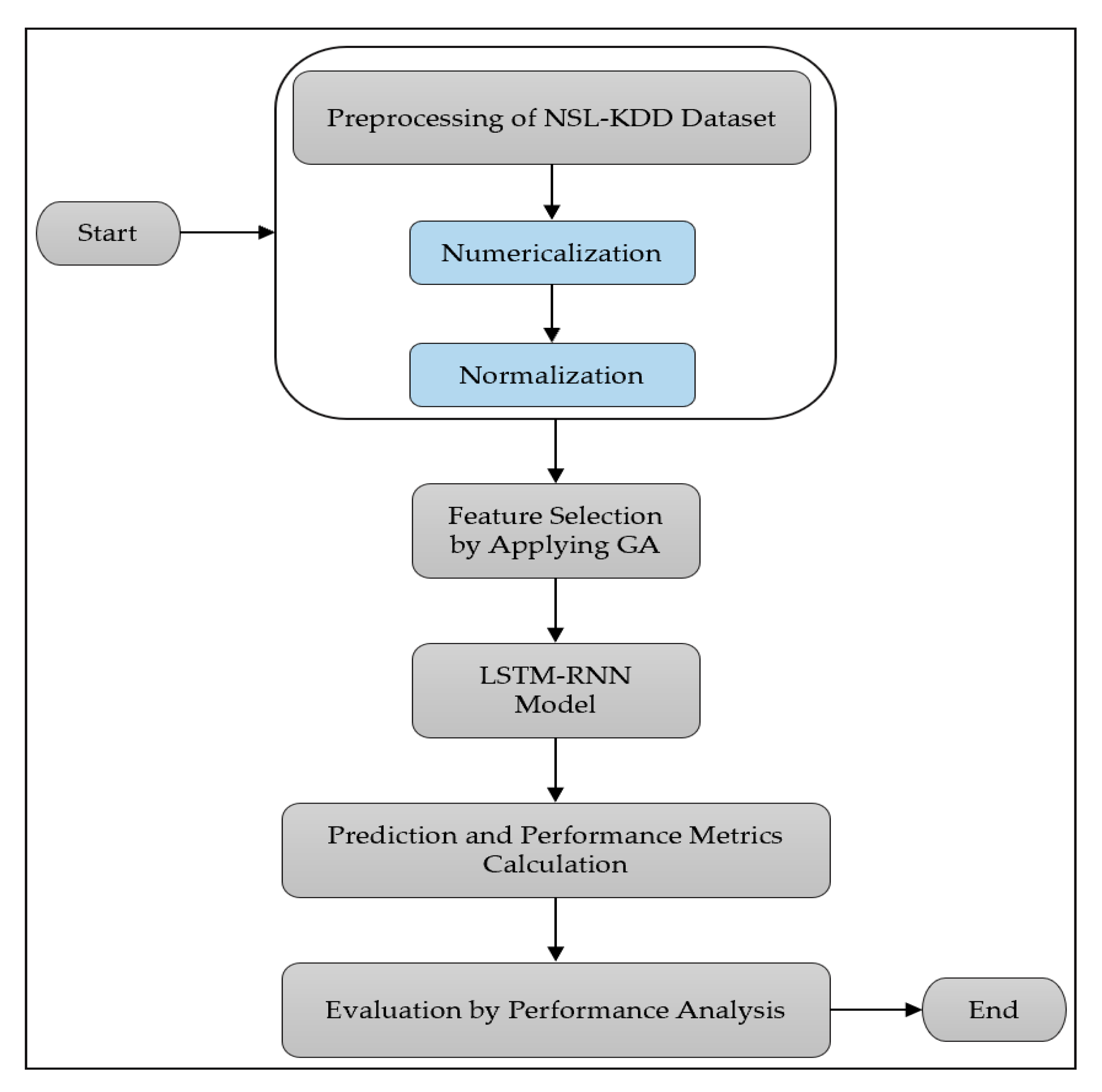
4. LSTM-RNN NIDS with a Genetic Algorithm

This section describes the LSTM-RNN NIDS with the feature-selection GA. The RNN is the basic model, and a LSTM network is used to achieve a high detection rate.

In this research, the training dataset was used to train the classifier, and the testing dataset was then used to measure the accuracy of the classifier. Two types of classifications were conducted: binary and multi-class. Normal and anomaly are the two classes in binary classification, whereas normal, denial of service (DoS), probe, user-to root (U2R), and remote-to-local (R2L) are the five categories detected using multi-class classification.

The classification metrics considered in this research are accuracy, precision, recall, f-score, true positive rate, and false-positive rate. The confusion matrix was calculated to show the records of true positive, true negative, false positive, and false negative records achieved in each model.

The LSTM-RNN models were designed with 5, 10, 20, 40, 60, 80, and 100 neurons in the hidden layers. Python 3.7 with the scikit-learn, TensorFlow, and Keras packages was used to develop the programs along with other Python open-source libraries.

4.1. LSTM-RNN Classifier with GA Architecture

Figure 3 shows the following steps performed for classifying network attacks using the LSTM-RNN classifier along with the GA.

Step 1: Data Preprocessing

Numericalization: Our training and testing datasets include 38 numeric features and three non-numeric features. We must make all the features numeric to apply them the model, so we converted the non-numeric features, protocol-type, service, and flag, into numerals. There were three values in the protocol type, 70 values in service and 11 values in flag features. In transforming all non-numeric features, we mapped 41 features into 122 (= 38 + 3 + 70 + 11) features [15].

To transform the categorical features into binary features, we first transformed the features into integers using LabelEncoder, a scikit-learn package. Then the integers were passed to One-Hot-Encoder to transform them into binary features. The One-Hot-Encoder is a matrix of integers, which represent different sub-categories of categorical features. The output is a sparse matrix. Each column of the output matrix corresponds to one possible value of one feature. The values of the input features have the range [0, n].

Normalization: Some features in the feature space, such as duration, src_bytes, and dst_bytes, have a very large difference between the maximum and minimum values. We applied a logarithmic scaling method to map to the range [0, 1] [15].

Normalization is not required for every dataset, but a dataset like NSL-KDD, where the features have different ranges of values, will require normalizing the values. Normalization changes the values of a dataset to a common scale. If the features do not have a similar range of values, then the gradient descents may take too long to converge. By normalizing, we can assure that the gradient descents can converge more quickly. An added benefit is that normalizing data can also increase the accuracy of a classifier.

Step 2: Feature Selection

Feature selection from the dataset is the process of finding the most relevant feature-set for the future predictive model implementation. This technique was used to identify and remove the unneeded, redundant, and irrelevant features that do not contribute or decrease the accuracy of the future predictive model implementation for the classification.

Optimal feature selection is one of the most important tasks in developing an excellent NIDS because some features can bias the classifier to identify a particular class, and that may increase the amount of misclassification. To minimize the misclassification rate, to minimize the training time, and to maximize the accuracy of the classifier, we have applied a GA in our experiment. Using a GA, we have obtained an optimal subset of 99 features from the original 122 features. After applying the GA, insignificant data are removed from the original features set. The GA selects only a subset of relevant features. Accuracy is used as the fitness function in this research. We have calculated the maximum, minimum and average accuracy of the training dataset according to their labels. The GA provided a set of solutions by performing recombination and mutation of the features and selected the features with maximum, minimum, and average accuracy. The subset of features that gives the maximum accuracy was selected as the optimal feature set. We then prepared our training and testing datasets with this optimal feature set.

The flow-chart of the GA implementation is shown in Figure 4.

The GA is a heuristic optimization method and it was implemented to find the best feature-set from the NSL-KDD datasets using the DEAP (distributed Evolutionary Algorithms in Python) evolutionary computation framework [32].

Initialize the population: The NSL-KDD datasets were mapped into 122 features in this experiment. The GA initializes the population of 10 individual feature-sets, each time randomly selected from the total 122 features. Each of the 10 individual feature-sets is represented as a feature vector with 122 attributes. Each attribute from the feature-set contains either a value 1 that represents that the feature is included in the individual, or a value 0 that represents the feature is not included in the individual.

Fitness value assignment: After the initialization of the population, the GA assigns the fitness for each individual feature-set. Here the logistic regression (LR) is used for training the model. The LR model gets trained from each individual feature-set and evaluates the selection error. The lowest selection error represents the highest fitness. The GA ranks each individual feature-set according to its fitness.

Selection of individual for the next generation: After the fitness value assignment, the selection operator chooses the individuals that recombine later for the next generation. The selection operator selects the individuals according to their fitness levels. The number of selected individuals is N/2, N being the population size; i.e., almost half of the individuals will get selected in this step.

Crossover: In this phase, the GA recombines the selected individuals to generate a new population from almost half of the population already selected from the previous steps, although, the total number of features in the new population will remain the same. Here the GA chooses the best combination of feature-set from the N/2 individuals through uniform crossover method.

Mutation: The GA performs mutation to diversify the population and to prevent premature convergence. The GA flips the value of the attributes of the input individual and returns the new individual. In this experiment, the probability of each attribute to be flipped is set to 0.05. The introduction of a very low mutation probability helps the GA to increase the search ability over the individuals to form a diverse population of individual features-sets. It also prevents the drastic drop in the local minimum on the GA feature selection.

Final decision and termination: If 10 generations have been processed, the GA will select the individual with the highest predictive feature-set selection, and then terminate. Alternatively, the GA will continue to the “fitness value assignment” phase to produce the next generation until the GA makes a final decision on the highest predictive feature-set selection before the termination.

In our experiment, we identified a set of 70 unique features using the GA on the training dataset. Additionally, we obtained a set of 66 unique features by using the GA on the testing dataset (with the label removed). Finally, we prepared the feature sets of 99 features as the union of the training (70 features) and testing (66 features) subsets. Figure 5 represents the set of 99 features that we obtained by applying the GA.

We observed that most of the features selected by the GA are from service or flag categories. This is hardly surprising, as most of the features are of these two types. Protocol type is also a significant feature type. The GA selects most of the unique features which can predict an attack type, so most of the features in the optimal features set are from service, protocol_type, and flag categories. Some of the other features besides service, protocol_type, and flag are also unique with having a large amount of potential value, so the GA selects them too.

Step 3: LSTM-RNN Model Construction

To build the LSTM-RNN model, first we selected hyper-parameters and optimizers for both binary and multi-class classification. We determined the following hyper-parameters: batch size, the number of epochs, learning rate, dropout, and activation function.

• Batch size is the number of training records in one forward and one backward pass.
• An epoch means one forward and one backward pass of all the training examples.
• Learning rate is the proportion of the weights that are updated during the training of the LSTM-RNN model. It can be chosen from the range [0.0–1.0].
• Dropout is a regularization technique, where randomly selected neurons are ignored during training. The selected neurons are temporarily removed on the forward pass.
• The activation function converts an input signal of a node in a neural network to an output signal, which is then used as the input of the next hidden layer and so on. To find the output of a layer, we calculated the sum of the products of inputs and their corresponding weights, applied the activation function to that sum, and then fed that output as an input to the next layer.

A suitable optimizer plays a very crucial part in classification. From various available optimizers, we selected stochastic gradient descent (SGD) for multiclass classification and the Adam optimizer for binary classification. SGD provides a lower computational cost than other gradient descent optimizers used in multiclass classification. Because other optimizers, such as the batch gradient descent and mini-batch gradient descent optimizers, use all the training samples for completing one iteration, they are computationally expensive to use. The advantage of SGD is that it uses only one batch for each iteration.

The Adam optimizer is easy to implement and computationally efficient because the decision is in binary and it requires less memory to implement.

Step 4: Prediction and performance metrics calculation

After fitting the model using the training dataset and testing dataset, we obtained the testing accuracy rate and loss value of the classifier. The testing dataset is used as a validation set to get an unbiased estimate of accuracy during the learning process. Then we used the predict_classes module of Keras to get the prediction matrix of the model; that is the classes predicted by the model. At this point, the expected classes have been defined in the original KDDTest+ dataset and the predicted classes. Next, we calculated the classification metrics such as precision, recall, f-score, true positive rate (TPR), false-positive rate (FPR), and confusion matrix from the expected and predicted classes matrix. These metrices are explained in Appendix A.

Step 5: Evaluation by performance analysis

We performed Step 4 for both SVM and RF classifiers and then evaluated the performances of SVM, RF, and LSTM-RNN by comparing the metrics.

4.2. Experiment Environment Setup

TensorFlow and Keras were used to implement the LSTM-RNN model, and scikit-learn was used to implement SVM and RF. Two types of classifications have been performed to study the performance of the LSTM-RNN model: binary and multi-class/5-category. Binary classification gives normal and anomaly detection results and multi-class/5-category classification gives normal, DoS, Probe, R2L and L2R attack detection results. These two types of classifications have been performed using a set of 122 features and an optimal set of 99 features. The optimal set of 99 features was obtained using the genetic algorithm.

To prevent overfitting in LSTM-RNN, we introduced several dropout amounts during the training of the model. While experimenting with two and three hidden layers, we randomly selected 1% of the neurons to drop out. We dropped out 10%–15% of the neurons while experimenting with four and five hidden layers. A dropout of 20%–30% was performed while experimenting with six, seven, and eight hidden layers. We have adjusted the dropout percentage for the hidden layers through several executions of the same experiment. We executed each experiment at least four times in different machines to adjust the dropout amount in the hidden layers. Those determined dropout amounts are given in

Table 4. Hyper-parameters of experiments.

Hyper-Parameter	Binary Classification	Multi-Class Classification
Learning Rate	0.01	0.01
Dropout	0.01, 0.15, 0.2, 0.3	0.01, 0.15, 0.2, 0.3
Activation function	sigmoid	Softmax
Optimizer	adam	SGD
Epoch	500	500
Batch size	50	50
Loss function	binary_crossentropy	categorical_crossentropy

.

We have implemented the default Linear SVM classifier function of scikit-learn using C-Support Vector Classification. We selected the Linear Kernel for SVM implementation.

In addition, we have implemented the RF using the default RandomForest classifier function of scikit-learn. The RandomForest function is implemented with n_estimators = 100 by default.

Hyper-Parameter Setup for Experiments with the LSTM-RNN Model

We have experimented with the LSTM-RNN model by using 5, 10, 20, 40, 60, 80, and 100 neurons in hidden layers for both binary and multi-class classification experiments. Hyper-parameters selected for the binary and multi-class classification experiments are shown in Table 4. The size of the hidden layers of the experiment is shown in

Table 5. The size of the hidden layer.

No. of Neurons in Hidden Layers	Number of the Hidden Layers
5	2
10	3
20	4
40	5
60	6
80	7
100	8

.

5. Experimental Results

In this section, we present the classification performance of the LSTM-RNN classifier according to accuracy, precision, recall, f-score, TPR and FPR on 5, 10, 20, 40, 60, 80, and 100 neurons in the hidden layers, respectively. The classification performance is analyzed for both binary and 5-class classification. For 5-class classification, the classes include normal, DoS, probe, U2R, and R2L attacks, while for binary classification, the classes include normal and anomaly. We also compared the performance of LSTM-RNN with traditional machine learning approaches such as SVM and RF using the same mixed feature sets. We compared the performance using the 122-feature set and the 99-feature set, which were obtained with the genetic algorithm.

5.1. Classification Results of the LSTM-RNN Classifier

The binary and multiclass classification results of the LSTM-RNN classifier are presented below.

5.1.1. Classification Results Using all Features

Table 6. Binary classification performance results using 122 features.

No. of Neurons in Hidden Layers	Accuracy		Precision	Recall	f1-Score	TPR	FPR
	Training %	Testing %
5	99.88	96.51	0.97	0.97	0.97	0.944	0.007
10	99.90	96.29	0.96	0.96	0.96	0.944	0.012
20	99.90	96.41	0.96	0.96	0.96	0.942	0.006
40	99.89	96.28	0.95	0.96	0.96	0.943	0.011
60	99.88	96.25	0.96	0.96	0.96	0.939	0.006
80	99.86	96.04	0.96	0.96	0.96	0.936	0.007
100	99.85	95.94	0.96	0.96	0.96	0.934	0.008

and

Table 7. Multi-class classification performance results using 122 features.

No. of Neurons in Hidden Layers	Accuracy		Precision	Recall	f1-Score	TPR	FPR
	Train %	Test %
5	96.00	85.65	0.86	0.86	0.85	0.765	0.023
10	98.00	78.13	0.80	0.78	0.73	0.630	0.019
20	98.70	76.61	0.72	0.74	0.69	0.589	0.060
40	99.89	82.42	0.87	0.82	0.81	0.697	0.008
60	99.87	82.68	0.87	0.83	0.81	0.707	0.015
80	99.84	81.33	0.87	0.81	0.79	0.685	0.017
100	99.85	82.06	0.85	0.82	0.81	0.689	0.006

show the performance of the LSTM-RNN classifier for binary classification and multi-class classification, respectively, while using the 122-dimensional feature space.

From Table 6, we observed that, in binary classification using all features, the highest testing accuracy obtained is 96.51% and the highest training accuracy obtained is 99.88%, in both cases using only five neurons in the hidden layers.

From Table 7, we observe that, in multi-class classification using all features, the highest testing accuracy obtained is 82.68% and the highest training accuracy obtained is 99.87%, in both cases using 60 neurons in the hidden layers.

5.1.2. Classification Results Using Optimal Feature Set

Table 8. Binary classification performance results using 99 features.

No. of Neurons in Hidden Layers	Accuracy		Precision	Recall	f1-Score	TPR	FPR
	Training (%)	Testing (%)
5	99.99	99.83	1.00	1.00	1.00	0.999	0.004
10	99.99	99.81	1.00	1.00	1.00	0.999	0.003
20	99.99	99.80	1.00	1.00	1.00	0.999	0.004
40	99.99	99.91	1.00	1.00	1.00	0.999	0.003
60	99.99	99.91	1.00	1.00	1.00	0.999	0.004
80	99.99	99.84	1.00	1.00	1.00	0.999	0.003
100	99.99	99.82	1.00	1.00	1.00	0.999	0.007

and

Table 9. Multi-class classification performance results using 99 features.

No. of Neurons in Hidden Layers	Accuracy		Precision	Recall	f1-Score	TPR	FPR
	Training (%)	Testing (%)
5	98.4	87.77	0.92	0.88	0.86	0.792	0.009
10	98.2	82.58	0.87	0.83	0.81	0.751	0.076
20	98.3	67.65	0.72	0.68	0.63	0.472	0.053
40	98.6	87.62	0.90	0.88	0.86	0.794	0.015
60	99.0	89.74	0.93	0.90	0.89	0.825	0.006
80	99.0	93.88	0.96	0.94	0.94	0.896	0.005
100	99.8	91.39	0.93	0.89	0.89	0.810	0.007

show the performance of the LSTM-RNN classifier after applying the genetic algorithm with 99 prominent features in binary and multiclass classification, respectively.

From Table 8, we observe that, in binary classification using 99 optimal features, the highest testing accuracy obtained is 99.91% and the highest training accuracy obtained is 99.99%, in both cases using 40 neurons in the hidden layers.

From Table 9, we observed that, in multi-class classification using the optimal set of 99 features, the highest testing accuracy obtained is 93.88% and the highest training accuracy obtained is 99.0%, in both cases using 80 neurons in the hidden layers.

5.2. Performance Comparison between Classifiers

The binary and multi-class classification performance comparisons between the LSTM-RNN classifier and the SVM and RF classifiers are presented below.

5.2.1. Performance Comparison Using All Features

Table 10. Performance comparison for binary classification using 122 features.

Method	Testing Accuracy (%)	Precision	Recall	f1-Score	TPR	FPR
SVM	92.90	0.94	0.93	0.93	0.876	0.002
Random forest	99.99	1.00	1.00	1.00	0.999	0.0001
LSTM-RNN	96.51	0.97	0.97	0.97	0.944	0.007

and

Table 11. Performance comparison for multi-class classification using 122 features.

Method	Testing Accuracy (%)	Precision	Recall	f1-Score	TPR	FPR
SVM	67.20	0.43	0.42	0.41	0.478	0.071
Random forest	80.70	0.90	0.55	0.53	0.661	0.001
LSTM-RNN	82.68	0.87	0.83	0.81	0.707	0.015

show the performance results of the SVM, RF, and LSTM-RNN classifiers for binary classification and multi-class classification, respectively, when using 122 features.

From Table 10 we observed that, LSTM-RNN performed better than the SVM. However, RF is the best in the binary classification experiments using all features. However, LSTM-RNN was able to obtain 96.51% testing accuracy with a TPR of 0.944.

Table 11 shows that LSTM-RNN provides the best testing accuracy of 82.68% among the other classifiers, where SVM gives 67.20% and RF gives 80.70% testing accuracy in multiclass classification experiments using all features. The TPR (0.707) is also higher for LSTM-RNN than SVM and RF.

5.2.2. Performance Comparison Using Optimal Features

Table 12. Performance comparison for binary classification using 99 features.

Method	Testing Accuracy (%)	Precision	Recall	f1-Score	TPR	FPR
SVM	99.90	0.99	0.99	0.99	0.999	0.001
Random forest	99.99	1.00	1.00	1.00	1.00	0.0001
LSTM-RNN	99.91	1.00	1.00	1.00	0.999	0.003

and

Table 13. Performance comparison for multi-class classification using 99 features.

Method	Testing Accuracy %	Precision	Recall	f1-Score	TPR	FPR
SVM	68.10	0.70	0.43	0.44	0.480	0.053
Random forest	84.90	0.89	0.59	0.57	0.735	0.0001
LSTM-RNN	93.88	0.96	0.94	0.94	0.896	0.005

show the performance results of SVM, random forest and LSTM-RNN classifiers for both binary and multi-class classification respectively when using the 99 optimal features set.

Table 12 shows that using the 99 optimal features set, LSTM-RNN, SVM, and RF give the similar testing accuracy, around 99.9%. In binary classification with an optimal features set, these three classifiers perform almost similar.

In Table 13, we observe that in multiclass-classification experiment, LSTM-RNN gives the best testing accuracy of 93.88% among all the experimented classifiers while using the 99 optimal features set. SVM provides 68.10% and RF provides 84.90% testing accuracy. The TPR (0.896) is also higher for LSTM-RNN comparing with SVM and RF in that experiment.

6. Discussion

In this research, we obtained binary classification results and 5-class classification results. In both categories of classification, we applied a genetic algorithm for feature selection. In this section, we discuss the outcomes and findings of our experiments.

6.1. Binary Classification

In binary classification, while using 122 features, we obtained an accuracy of 96.51% for KDDTest+ and an accuracy of 99.88% for the KDDTrain+ dataset. We obtained this high detection rate while using only five neurons in the hidden layers. The TPR and FPR are 0.944 and 0.007, respectively.

After applying the genetic algorithm and using the optimal set of 99 features, we were able to obtain an increased accuracy of 99.91% for KDDTest+ and 99.99% for KDDTrain+ using 40 neurons in the hidden layers with a TPR of 0.999 and FPR of 0.003. We were able to enhance the accuracy by more than 3%. We were able to obtain 99.83% testing accuracy using only five neurons, which is very similar to the highest accuracy of our experiment. Thus, after applying the GA, we could reach the maximum testing accuracy using a small LSTM-RNN network. By using this small network architecture, we were able to minimize the running time as well.

In this experiment, we observed that RF gives the highest testing accuracy in binary classification. Because it is easy to build random binary decision trees if the classes are well defined by the features. The random trees are usually split into different subsets. Then it searches for the best outcome from the random subsets. In the experiment, we implemented the default RandomForest classifier function of scikit-learn which combines hundreds of decision tress. In each tree, there are two final predictions to make, either normal (labeled as 0) or anomalous (labeled as 1).

In this experiment, LSTM-RNN was implemented considering several parameters such as dropout, batch-size, epochs, optimizers etc. The performance of the classifier was biased by those parameters. Thus, the performance of LSTM-RNN in binary classification is slightly less than RF.

The confusion matrices for binary classification on KDDTest+ using 122 features and 99 features are presented in

Table 14. The confusion matrices of binary classification on KDDTest+ (122 features vs. 99 features).

	Predicted Class
	Using 122 Features		Using 99 Features
Actual Class	Anomaly	Normal	Anomaly	Normal
Anomaly	12115	718	12831	2
Normal	68	9643	18	9693

We can observe that the use of the genetic algorithm decreased the amount of misclassification. The numbers of correctly classified records are shown in the gray boxes.

6.2. Multi-Class Classification

In multi-class classification while using 122 features, we obtained 82.68% accuracy for KDDTest+ and 99.87% accuracy for the KDDTrain+ dataset. We obtained this high detection rate while using 60 neurons in the hidden layers. The TPR and FPR are 0.707 and 0.015, respectively.

After applying the genetic algorithm and obtaining the optimal set of 99 features, we obtained an increased accuracy of 93.88% for KDDTest+ and 99.0% for KDDTrain+ with a TPR of 0.896 and a FPR of 0.005 while using 80 neurons in the hidden layers. The accuracy is more than 10% higher than using all features. The experiment using the genetic algorithm also reduced the training and testing times. From Table 7 we see that we have already obtained an accuracy of 82.68% by using only 10 neurons in the hidden layers after using the GA.

The confusion matrices of the multi-class classification on KDDTest+ using 122 features and 99 features are presented in

Table 15. The confusion matrices of multi-class classification on KDDTest+ (122 features vs. 99 features).

	Predicted Class
	Using 122 Features					Using 99 Features
Actual Class	Normal	DoS	Probe	R2L	U2R	Normal	DoS	Probe	R2L	U2R
Normal	9562	147	2	0	0	9660	50	1	0	0
DoS	795	6143	522	0	0	0	7417	43	0	0
Probe	5	157	2232	25	2	0	46	2271	79	25
R2L	250	7	1907	686	35	0	1	877	1770	237
U2R	20	4	3	23	17	1	0	0	20	46

. There are 60 neurons in the hidden layer. We can observe that the use of a genetic algorithm decreased the number of misclassifications. The number of correctly classified records is shown in the gray boxes.

Table 16. Results of the evaluation metrics for multi-class classification using 122 features and 60 neurons in the hidden layers.

Normal/Attack Type	Precision	Recall	f1-Score	Accuracy (%)
Normal	0.90	0.98	0.94	98.47
DoS	0.95	0.82	0.88	82.35
Probe	0.48	0.92	0.63	92.19
R2L	0.93	0.24	0.38	23.78
U2R	0.31	0.25	0.28	25.37

shows the best results of the evaluation metrics for each individual class of multi-class classification experiment using 122 features. From this table, we can see that the accuracy rate for R2L and U2R classes is comparatively lower than that for the other classes. This is due to the small number of training records for U2R and R2L.

Table 17. Results of the evaluation metrics for multi-class classification using 99 features and 80 neurons in the hidden layers.

Normal/Attack Type	Precision	Recall	f1-Score	Accuracy (%)
Normal	1.00	0.99	1.00	99.47
DoS	0.99	0.99	0.99	99.43
Probe	0.71	0.94	0.81	93.80
R2L	0.95	0.61	0.74	61.35
U2R	0.15	0.69	0.25	68.66

shows the best results for the evaluation metrics for each individual class of multi-class classification experiments using 99 features and 80 neurons in the hidden layers. It also shows that using the GA enhanced the classification accuracy of the R2L and U2R classes compared with using 122 features.

In [22], the researchers proposed a deep learning approach, self-taught learning, which can achieve a high accuracy of 88.39% for binary classification and 79.10% for 5-class classification. Based on the evaluation using the KDDTrain+ dataset, we found the performance of LSTM-RNN is comparable to the best results obtained in several previous works [16,22]. In [20], the researchers applied LSTM-RNN on the KDD Cup’ 99 datasets and obtained 93.82% accuracy in 5-class classification by using a 0.1 learning rate and 1000 epochs. In our research using LSTM-RNN with the GA, we were able to obtain 99.99% training accuracy and 99.91% testing accuracy in the binary classification experiment. Moreover, we obtained 99% training accuracy and 93.88% testing accuracy in the five-class classification experiment.

7. Conclusions

In this paper, we compared different classifiers on the NSL-KDD dataset for both binary and multi-class classification. We considered SVM, random forest, and the LSTM-RNN model. We have shown that our proposed model produced the highest accuracy rate of 96.51% and 99.91% for binary classification using 122 features and an optimal set of 99 features, respectively. The LSTM-RNN obtained higher accuracy than the SVM in binary classification. However, random forest was the best classifier among all in that case. However, using the 99-feature set, we were able to get testing accuracy similar to that of RF.

In addition, we achieved a testing accuracy of 82.68% using the 122-feature set and 93.88% accuracy while using the 99-feature set in multi-class classification. When compared with the SVM and random forest, LSTM-RNN performed the best in multiclass classification experiments. Our LSTM-RNN-with-GA model achieved a 10% higher accuracy than random forest in that experiment. Using the GA improves the performance of the LSTM-RNN classifier significantly. Finally, we conclude that LSTM-RNN is suitable for large datasets. With small datasets having few features, the performance of LSTM-RNN is not very noticeable. However, enhanced with the GA, LSTM-RNN performs comparatively better than traditional machine learning approaches.

In this research, all the experiments were executed using a Windows platform. In this experiment, we did not record the training time. In future, we will execute all the experiments in a GPU-based system for obtaining a faster training time. Another future work should include using a more recent dataset such as UNSW-NB15 to verify the efficiency of the LSTM-RNN model. Another example for future work will be developing a framework for collecting real-time network data, labeling the dataset with expert knowledge, and then applying the proposed LSTM-RNN classifier on that dataset. Additionally, we will extend our experiments for comparing the performance of LSTM_RNN-with-GA to those of other deep-learning approaches, such as CNN-LSTM, STL, deep belief network (DBN), on the latest datasets.

References

1. Denning, D.E. An intrusion-detection model. IEEE Trans. Softw. Eng. 1987, 13, 222–232. [Google Scholar] [CrossRef]
2. Peddabachigari, S.; Abraham, A.; Thomas, J. Intrusion Detection Systems Using Decision Trees and Support Vector Machines. Int. J. Appl. Sci. Comput. 2004, 11, 118–134. [Google Scholar]
3. Rai, K.; Devi, M.S.; Guleria, A. Decision Tree Based Algorithm for Intrusion Detection. Int. J. Adv. Netw. Appl. 2016, 7, 2828–2834. [Google Scholar]
4. Ingre, B.; Yadav, A.; Soni, A. K Decision Tree-Based Intrusion Detection System for NSL-KDD Dataset. In Proceedings of the International Conference on Information and Communication Technology for Intelligent Systems, Ahmedabad, India, 25–26 March 2017. [Google Scholar] [CrossRef]
5. Farnaaz, N.; Jabbar, M.A. Random Forest Modeling for Network Intrusion Detection System. Procedia Comput. Sci. 2016, 89, 213–217. [Google Scholar] [CrossRef] [Green Version]
6. Alom, M.Z.; Taha, T.M. Network intrusion detection for cybersecurity using unsupervised deep learning approaches. In Proceedings of the IEEE National Aerospace and Electronics Conference (NAECON), Dayton, OH, USA, 27–30 June 2017. [Google Scholar] [CrossRef]
7. Yuan, Y.; Huo, L.; Hogrefe, D. Two Layers Multi-class Detection Method for Network Intrusion Detection System. In Proceedings of the IEEE Symposium on Computers and Communications (ISCC), Heraklion, Greece, 3–6 July 2017. [Google Scholar] [CrossRef]
8. Gurav, R.; Junnarkar, A.A. Classifying Attacks in NIDS Using Naïve- Bayes and MLP. Int. J. Sci. Eng. Technol. Res. (IJSETR) 2015, 4, 2440–2443. [Google Scholar]
9. Tangi, S.D.; Ingale, M.D. A Survey: Importance of ANN-based NIDS in Detection of DoS Attacks. Int. J. Comput. Appl. 2013, 83. [Google Scholar] [CrossRef]
10. Szegedy, C.; Toshev, A.; Erhan, D. Deep Neural Networks for Object Detection. In Proceedings of the 26th International Conference on Neural Information Processing Systems—Volume 2; Curran Associates Inc.: Red Hook, NY, USA, 2013; pp. 2553–2561. [Google Scholar]
11. Wang, M.; Huang, Q.; Zhang, J.; Li, Z.; Pu, H.; Lei, J.; Wang, L. Deep Learning Approaches for Voice Activity Detection. In Proceedings of the International Conference on Cyber Security Intelligence and Analytics, Shenyang, China, 21–22 February 2019; pp. 816–826. [Google Scholar]
12. Tang, T.A.; Mhamdi, L.; McLernon, D.; Zaidi, S.A.R.; Ghogho, M. Deep Learning Approach for Network Intrusion Detection in Software-Defined Networking. In Proceedings of the 2016 International Conference on Wireless Networks and Mobile Communications, Fez, Morocco, 26–29 October 2016. [Google Scholar] [CrossRef]
13. Arora, K.; Chauhan, R. Improvement in the Performance of Deep Neural Network Model using learning rate. In Proceedings of the Innovations in Power and Advanced Computing Technologies (i-PACT), Vellore, India, 21–22 April 2017. [Google Scholar] [CrossRef]
14. Tang, T.A.; Mhamdi, L.; McLernon, D.; Zaidi SA, R.; Ghogho, M. Deep Recurrent Neural Network for Intrusion Detection in SDN-based Networks. In Proceedings of the 4th IEEE International Conference on Network Softwarization (NetSoft), Montreal, QC, Canada, 25–29 June 2018. [Google Scholar] [CrossRef] [Green Version]
15. Yin, C.; Zhu, Y.; Fei, J.; He, X. A Deep Learning Approach for Intrusion Detection Using Recurrent Neural Networks. IEEE Access 2017, 5, 21954–21961. [Google Scholar] [CrossRef]
16. Vinayakumar, R.; Soman, K.P.; Poornachandran, P. Applying convolutional neural network for network intrusion detection. In Proceedings of the International Conference on Advances in Computing, Communications, and Informatics (ICACCI), Udupi, India, 13–16 September 2017. [Google Scholar] [CrossRef]
17. Zhao, G.; Zhang, C.; Zheng, L. Intrusion Detection Using Deep Belief Network and Probabilistic Neural Network. In Proceedings of the IEEE International Conference on Computational Science and Engineering (CSE) and IEEE International Conference on Embedded and Ubiquitous Computing (EUC), Guangzhou, China, 21–24 July 2017. [Google Scholar] [CrossRef]
18. Kim, J.; Kim, J.; Thu HL, T.; Kim, H. Long Short-Term Memory Recurrent Neural Network Classifier for Intrusion Detection. In Proceedings of the International Conference on Platform Technology and Service (PlatCon), Jeju, Korea, 15–17 February 2016. [Google Scholar] [CrossRef]
19. Staudemeyer, R.C. Applying long short-term memory recurrent neural networks to intrusion detection. S. Afr. Comput. J. 2015, 56, 136–154. [Google Scholar] [CrossRef]
20. Meng, F.; Fu, Y.; Lou, F.; Chen, Z. An Effective Network Attack Detection Method Based on Kernel PCA and LSTM-RNN. In Proceedings of the International Conference on Computer Systems, Electronics, and Control (ICCSEC), Dalian, China, 25–27 December 2017. [Google Scholar] [CrossRef]
21. Staudemeyer, R.C.; Omlin, C.W. Evaluating performance of long short-term memory recurrent neural networks on intrusion detection data. In Proceedings of the South African Institute for Computer Scientists and Information Technologists Conference; Association for Computing Machinery: New York, NY, USA, 2013; pp. 218–224. [Google Scholar] [CrossRef]
22. Javaid, A.; Niyaz, Q.; Sun, W.; Alam, M. A Deep Learning Approach for Network Intrusion Detection System. In Proceedings of the 9th EAI International Conference on Bio-inspired Information and Communications Technologies (BIONETICS), New York, NY, USA, 24 May 2016; pp. 21–26. [Google Scholar] [CrossRef] [Green Version]
23. Hindy, H.; Brosset, D.; Bayne, E.; Seeam, A.; Tachtatzis, C.; Atkinson, R.; Bellekens, X. A Taxonomy and Survey of Intrusion Detection System Design Techniques, Network Threats and Datasets. arXiv 2018, arXiv:1806.03517. [Google Scholar]
24. Artificial Neural Network–Wikipedia. Available online: https://en.wikipedia.org/wiki/Artificial_neural_network (accessed on 29 April 2020).
25. Recurrent Neural Network-Wikipedia. Available online: https://en.wikipedia.org/wiki/Recurrent_neural_network (accessed on 29 April 2020).
26. Hochreiter, S.; Bengio, Y.; Frasconi, P.; Schmidhuber, J. Gradient Flow in Recurrent Nets: The Difficulty of Learning Long-term Dependencies. In A Field Guide to Dynamical Recurrent Neural Networks; IEEE Press: Piscataway, NJ, USA, 2001; pp. 237–243. [Google Scholar] [CrossRef]
27. Williams, R.J.; Zipser, D. Gradient based learning algorithms for recurrent networks and their computational complexity. In Backpropagation: Theory, Architectures, and Applications; Lawrence Erlbaum Associates: Hillsdale, NJ, USA, 1995; pp. 433–486. [Google Scholar]
28. Genetic Algorithms—Introduction. Available online: https://www.tutorialspoint.com/genetic_algorithms/genetic_algorithms_introduction.htm (accessed on 29 April 2020).
29. Tavallaee, M.; Bagheri, E.; Lu, W.; Ghorbani, A.A. A Detailed Analysis of the KDD CUP 99 Data Set. In Proceedings of the 2009 IEEE Symposium on Computational Intelligence for Security and Defense Applications, Ottawa, ON, Canada, 8–10 July 2009; pp. 1–6. [Google Scholar]
30. Dhanabal, L.; Shantharajah, S.P. A Study on NSL_KDD Dataset for Intrusion Detection System Based on Classification Algorithms. Int. J. Adv. Research Comput. Commun. Eng. 2015, 4, 446–452. [Google Scholar]
31. Hamid, Y.; Balasaraswathi, V.R.; Journaux, L.; Sugumaran, M. Benchmark Datasets for Network Intrusion Detection: A Review. Int. J. Netw. Secur. 2018, 20, 645–654. [Google Scholar] [CrossRef]
32. Evolutionary Tools. Available online: https://deap.readthedocs.io/en/master/api/tools.html (accessed on 29 April 2020).
Figure 1. A simple RNN.
Information 11 00243 g001
Figure 2. One cell in a basic LSTM network.
Information 11 00243 g002
Figure 3. Flow-chart of the LSTM-RNN classifier with GA.
Information 11 00243 g003
Figure 4. The flowchart of genetic algorithm implementation.
Information 11 00243 g004
Figure 5. Features set after applying the GA.
Information 11 00243 g005