Applications of Nonlinear Programming to the Optimization of Fractionated Protocols in Cancer Radiotherapy

Abstract

The present work of review collects and evidences the main results of our previous papers on the optimization of fractionated radiotherapy protocols. The problem under investigation is presented here in a unitary framework as a nonlinear programming application that aims to determine the optimal schemes of dose fractionation commonly used in external beam radiotherapy. The radiation responses of tumor and normal tissues are described by means of the linear quadratic model. We formulate a nonlinear, non-convex optimization problem including two quadratic constraints to limit the collateral normal tissue damages and linear box constraints on the fractional dose sizes. The general problem is decomposed into two subproblems: (1) analytical determination of the optimal fraction dose sizes as a function of the model parameters for arbitrarily fixed treatment lengths; and (2) numerical determination of the optimal fraction number, and of the optimal treatment time, in different parameter settings. After establishing the boundedness of the optimal number of fractions, we investigate by numerical simulation the optimal solution behavior for experimentally meaningful parameter ranges, recognizing the crucial role of some parameters, such as the radiosensitivity ratio, in determining the optimality of hypo- or equi-fractionated treatments. Our results agree with findings of the theoretical and clinical literature.

1. Introduction

The common goal in cancer treatments is to achieve the best compromise between treatment efficacy and safety. Among the methods for cancer management, fractionated radiotherapy has a major clinical role as a component of multi-modality therapy or even as the sole treatment modality. External beam radiation therapy (EBRT) is usually administered in daily fractions, and it aims to maximize the overall radiation damage to the tumor, while preserving the surrounding healthy tissue. At the same time, dose fractionation allows the repair of normal tissues while hindering the effects of tumor repopulation. Therefore, the determination of suitable radiation treatments is intrinsically associated to the solution of constrained optimization problems. Methods for radiotherapy optimization highly contribute to improving the outcome of cancer radiation treatment and have been the object of many studies in recent years. These methods span several techniques: from experimental techniques that use chemical agents enhancing the tumor response or reducing the normal tissue response [1,2], to empirical and/or numerical procedures for the optimization of protocols with respect to the fraction size and to the overall treatment time [3,4,5], up to model-based applications of optimal control providing the optimal time–dose scheme of radiation administration (EBRT) [6,7,8,9] or the optimal volume distributions of the radiation (intensity modulated radiotherapy, IMRT) [10,11].

Here, we overview the results of our work aimed to solve a general radiotherapy problem formulated in the framework of the optimization of time–dose fractionation protocols and based on the linear-quadratic (LQ) model of cell survival [6,12,13]. The LQ model expresses the relation between a single dose of radiation d (Gy) and the fraction of cells that survive the irradiation, S, as

$$S=\exp (-\alpha d-\beta d^2),$$

where the parameters $\alpha$ and $\beta$ represent the intrinsic radiosensitivity of the cell population. The linear term accounts for lethal non repairable DNA lesions, while the quadratic term represents the lethal effect of the misrepair of DNA double-strand breaks [14]. The argument of the exponential represents the effect of instantaneous cell killing following a single irradiation. However, when multiple radiation sessions are delivered other fractionation/protraction effects have to be taken into account, as done in the extended version of the LQ model proposed by Brenner et al. [15] (LQR model). Processes included in the LQR model are the compensatory repopulation owing to the regrowth of cells surviving irradiation, the repair of the radiation damage, and the resensitization mechanisms (i.e., redistribution of cells across the cell-cycle phases plus reoxygenation).

Many theoretical studies for radiotherapy optimization based on the LQ and LQR models have been proposed in the literature over the last 35 years. An up to date list of such interesting papers can be found in [9]. Here, we rather mention the “intriguing” scientific debate concerning the appropriateness of the LQ model for the description of the radiation response of cell populations, especially when large radiation doses are delivered. Indeed, recent technological advances in radiotherapy, such as IMRT or stereotactic body radiation therapy (SBRT), made possible the use of larger-than-conventional doses per fraction. Thus, the LQ model has been much discussed [16,17], but in the end accepted for two main reasons [18]: “(1) the standard LQ model is an approximation to more exact, but more complex models; (2) the LQ formalism works fine at doses per fraction below about 15–20 Gy, while at higher doses per fraction, more exact models are available and should be used”. A modified LQ model, specifically proposed to provide a better fit to data of radiation dose–response curves at high fractional doses, is the linear-quadratic-linear (LQ-L) model [19,20]. A more recent alternative to the LQ model providing an accurate estimation of the probability of tumor cell survival at high doses is based on accounting for the microdosimetric distribution in irradiated cells [21].

However, the LQ model continues to be extensively used in view of its simple formalism derived from biophysical principles and of its flexibility in representing the radiation response of different kinds of tissues for a clinically meaningful dose range. Some examples of very recent works (both theoretical and clinical) based on the LQ formalism are [22,23,24,25,26]. We also quote Brown [23] for the following very original defense of the LQ model “in a light-hearted manner”:

If you want to cure a tumor

Then finish radiation sooner

Give it $3\times 20$ Grays

And cut the time to just 5 days.

To figure dose just use LQ

With terms that are but two.

No need to add more bits

As the patient data already fits.

So keep it simple with nothing new

Just stick with straight LQ.

In Section 2, we formulate a general optimal radiotherapy problem assuming the LQ model for the description of cell radiation response. The first part of the present work (Section 3 and Section 4) is dedicated to the description of the analytical results obtained in [7,8] and related to the determination of the optimal fractionation of the radiation dose for a fixed (but arbitrary) treatment time. The second part (Section 5) concerns the problem of finding, besides the dose sizes, the optimal dose number, i.e., the optimal treatment length [9]. Numerical simulations for different tumor classes and for wide variations of the tumor parameters are presented in Section 6. Our computational results confirm recent findings of the theoretical and clinical literature showing the crucial role of some parameters, such as the tumor radiosensitivity ratio, in determining the optimality of different fractionated radiation schemes.

2. A general Optimal Radiotherapy Problem

We describe here the radiation-induced response of homogeneous cell populations by the LQ model [13] and we include the effects of lethal/sublethal instantaneous radiation damages and cell repopulation [5,15,27,28]. We consider fractionated radiation treatments in which the total dose is subdivided into n fractions administered as one fraction per day to the patient, leaving treatment breaks at the weekends according to the usual medical practice. Denoting by $d_i\ge 0,i=1,2,\dots ,n$, the fractional dose given at ith day, the cumulated effect of the instantaneous lethal damage is

$$E_1=\alpha \sum _{i=1}^n{d}_i+\beta \sum _{i=1}^n{d}_i^2,$$

(1)

where $\alpha$ and $\beta$ are the (strictly positive) LQ constants characterizing the intrinsic radiosensitivity of the population. The sublethal damage caused by incomplete repair is modeled as

$$E_2=2\beta {\mathrm{e}}^{-\gamma }\sum _{i=2}^n{d}_{i-1}{d}_i,$$

(2)

where $\gamma$ is the ratio of the inter-fraction time interval $\Delta$ and the repair time ${\tau }_R$. In Equation (2), the interaction between fractional doses more than one day apart is neglected since we assume $\Delta =24$ h and the literature reports ${\tau }_R\approx 4.0$ h as the typical value of the repair time [5].

Finally, cell repopulation is modeled by the exponential law with exponent

$$E_3=\frac{ln\left(2\right)}{T_P}\left(T-T_K\right)H(T-T_K),$$

(3)

where $T=T\left(n\right)$ is the overall treatment time (i.e., the number of days between the 1st and the last dose), $T_P$ is the population doubling time, $T_k$ is the starting time of compensatory proliferation (kick-off time), and $H(·)$ is the unitary step Heaviside function. Therefore, the fraction of surviving cells is

$$S=\exp (-E_1-E_2+E_3).$$

(4)

The model in Equation (4) is used to describe the response to radiation of the tumor, as well as of the early and late responding normal tissues. In the following, the quantities in Equations (1)–(3) related to the early and late tissues response are indexed by subscripts “e” and “l”, respectively.

Our goal is to minimize the fraction of surviving tumor cells S, and in particular its logarithm, initially with respect to the fractional dose sizes, then also with respect to their number. At the same time, suitable constraints on the maximal admissible damage to normal tissues have to be taken into account. Considering only the interaction between two consecutive fractions as non-negligible (${\gamma }_l=6$, ${\gamma }_e=48$ [5]), the constraints take the form

$$-\ln \left(S_e\right)=E_{1_e}+E_{2_e}-E_{3_e}\le C_e,-\ln \left(S_l\right)=E_{1_l}+E_{2_l}\le C_l,$$

(5)

where $C_e$ and $C_l$ denote the logarithmic maximal damage to the early and late responding tissue, respectively, and cell repopulation has been neglected for the late responding tissue. Additional constraints and specific simplifying assumptions are also considered and explained in detail in the following sections.

3. Optimization over a Single Week of Treatment

In the present section (as well as in Section 4), we assume that the period of radiation treatment administration consists of an integer number of weeks, $\omega$, and that treatment breaks are left at each weekend according to the standard medical practice. The total number of delivered fractions n and the overall treatment time T of the Equations (1)–(3) become

$$n=5\omega ,T=7\omega -3\mathrm{days}.$$

(6)

We assume that $\omega$, and then the overall treatment time T, is assigned. Then, the optimization problem considered here is to minimize the logarithm of the tumor surviving fraction S with respect to the fractional dose sizes only. Noting that $E_3$ does not depend on the doses, the problem is equivalent to that of minimizing the quantity $-E_1-E_2$. To simplify the optimization problem, we also assume that the cumulative damages to normal tissues, $C_e$ and $C_l$, are equi-distributed over the $\omega$ treatment weeks. This choice allows us to reformulate the problem over a single week of treatment, thus reducing the number of variables and, at the same time, to strengthen the constraints on the normal tissue damage. The obtained solution is then repeated for each treatment week.

Let us introduce the notations

$$\rho =\frac{\alpha }{\beta },{\rho }_e=\frac{{\alpha }_e}{{\beta }_e},{\rho }_l=\frac{{\alpha }_l}{{\beta }_l},h_e=\frac{C_e+E_{3e}}{\omega {\beta }_e},h_l=\frac{C_l}{\omega {\beta }_l}.$$

(7)

We observe that the radiosensitivity ratios are in general greater than 1 Gy either for tumors and for normal tissues. Typical values of $\rho$ reported in the literature range from about 2–3 to 50 Gy or more, whereas for the early and late normal tissues it is ${\rho }_e>{\rho }_l$ [4,29,30]. Let us now define the 5-dimensional vector d with components $d_i,i=1,\dots ,5$. The constraints in Equation (5) can be written in the form

$$g_e\left(d\right)={\rho }_e\sum _{i=1}^5{d}_i+\sum _{i=1}^5{d}_i^2+2{\mathrm{e}}^{-{\gamma }_e}\sum _{i=2}^5{d}_{i-1}{d}_i-h_e\le 0,$$

(8)

$$g_l\left(d\right)={\rho }_l\sum _{i=1}^5{d}_i+\sum _{i=1}^5{d}_i^2+2{\mathrm{e}}^{-{\gamma }_l}\sum _{i=2}^5{d}_{i-1}{d}_i-h_l\le 0,$$

(9)

and we can formulate the optimization problem to be solved over a single treatment week.

Problem 1.

Minimize the function

$$J\left(d\right)=-\rho \sum _{i=1}^5{d}_i-\sum _{i=1}^5{d}_i^2-2{\mathrm{e}}^{-\gamma }\sum _{i=2}^5{d}_{i-1}{d}_i$$

(10)

on the admissible set

$$\begin{array}{c}\hfill D=\{d\in {\mathbb{R}}^5|g_e\left(d\right)\le 0,g_l\left(d\right)\le 0,g_i\left(d\right)=-d_i\le 0,i=1,\dots ,5\}.\end{array}$$

(11)

It is important to note that Problem 1 certainly admits some optimal solutions in view of the Weierstrass theorem [31]. As the problem is not convex, the set of solution candidates is found by means of the Karush–Kuhn–Tucker necessary conditions of optimality. Theorems 1 and 2, reported here without demonstrations (see the complete proofs in [7]), illustrate how these candidates are structured, evidencing how they can be grouped into classes of equivalent, i.e., providing the same value of J, extremal solutions. The equivalence of the elements within each class is easily understood noticing that J, $g_e$, $g_l$ depends only on the quantities ${\sum }_{i=1}^5{d}_i$, ${\sum }_{i=1}^5{d}_i^2$, and ${\sum }_{i=2}^5{d}_{i-1}{d}_i$.

Theorem 1.

There are $2^5$ possible structures for the solutions d of Problem 1, including the trivial vector $d=0$. The non-trivial solutions may be grouped into 10 mutually exclusive classes, as reported in

Table 1. Classes of equivalent structures for the extremals of Problem 1.

Class	Representative	Number	Elements
$d^{\left(1\right)}$	$\left(A^{\left(1\right)}0000\right)$	5	$\left(A^{\left(1\right)}0000\right)$, $\left(0A^{\left(1\right)}000\right)$,
			$\left(00A^{\left(1\right)}00\right)$, $\left(000A^{\left(1\right)}0\right)$,
			$\left(0000A^{\left(1\right)}\right)$
$d^{\left(2\right)}$	$\left(0A^{\left(2\right)}0A^{\left(2\right)}0\right)$	6	$\left(A^{\left(2\right)}0A^{\left(2\right)}00\right)$, $\left(A^{\left(2\right)}00A^{\left(2\right)}0\right)$,
			$\left(A^{\left(2\right)}000A^{\left(2\right)}\right)$, $\left(0A^{\left(2\right)}0A^{\left(2\right)}0\right)$,
			$\left(0A^{\left(2\right)}00A^{\left(2\right)}\right)$, $\left(00A^{\left(2\right)}0A^{\left(2\right)}\right)$
$d^{\left(3\right)}$	$\left(A^{\left(3\right)}0A^{\left(3\right)}0A^{\left(3\right)}\right)$	1	$\left(A^{\left(3\right)}0A^{\left(3\right)}0A^{\left(3\right)}\right)$
$d^{\left(4\right)}$	$\left(0B^{\left(4\right)}{B}^{\left(4\right)}00\right)$	4	$\left(B^{\left(4\right)}{B}^{\left(4\right)}000\right)$, $\left(0B^{\left(4\right)}{B}^{\left(4\right)}00\right)$,
			$\left(00B^{\left(4\right)}{B}^{\left(4\right)}0\right)$, $\left(000B^{\left(4\right)}{B}^{\left(4\right)}\right)$
$d^{\left(5\right)}$	$\left(A^{\left(5\right)}0B^{\left(5\right)}{B}^{\left(5\right)}0\right)$	6	$\left(A^{\left(5\right)}0B^{\left(5\right)}{B}^{\left(5\right)}0\right)$, $\left(0A^{\left(5\right)}0B^{\left(5\right)}{B}^{\left(5\right)}\right)$,
			$\left(A^{\left(5\right)}00B^{\left(5\right)}{B}^{\left(5\right)}\right)$, $\left(B^{\left(5\right)}{B}^{\left(5\right)}0A^{\left(5\right)}0\right)$,
			$\left(B^{\left(5\right)}{B}^{\left(5\right)}00A^{\left(5\right)}\right)$, $\left(0B^{\left(5\right)}{B}^{\left(5\right)}0A^{\left(5\right)}\right)$
$d^{\left(6\right)}$	$\left(0C^{\left(6\right)}{D}^{\left(6\right)}{C}^{\left(6\right)}0\right)$	3	$\left(0C^{\left(6\right)}{D}^{\left(6\right)}{C}^{\left(6\right)}0\right)$, $\left(C^{\left(6\right)}{D}^{\left(6\right)}{C}^{\left(6\right)}00\right)$,
			$\left(00C^{\left(6\right)}{D}^{\left(6\right)}{C}^{\left(6\right)}\right)$
$d^{\left(7\right)}$	$\left(B^{\left(7\right)}{B}^{\left(7\right)}0B^{\left(7\right)}{B}^{\left(7\right)}\right)$	1	$\left(B^{\left(7\right)}{B}^{\left(7\right)}0B^{\left(7\right)}{B}^{\left(7\right)}\right)$
$d^{\left(8\right)}$	$\left(C^{\left(8\right)}{D}^{\left(8\right)}{C}^{\left(8\right)}0A^{\left(8\right)}\right)$	2	$\left(C^{\left(8\right)}{D}^{\left(8\right)}{C}^{\left(8\right)}0A^{\left(8\right)}\right)$, $\left(A^{\left(8\right)}0C^{\left(8\right)}{D}^{\left(8\right)}{C}^{\left(8\right)}\right)$
$d^{\left(9\right)}$	$\left(E^{\left(9\right)}{F}^{\left(9\right)}{F}^{\left(9\right)}{E}^{\left(9\right)}0\right)$	2	$\left(E^{\left(9\right)}{F}^{\left(9\right)}{F}^{\left(9\right)}{E}^{\left(9\right)}0\right)$, $\left(0E^{\left(9\right)}{F}^{\left(9\right)}{F}^{\left(9\right)}{E}^{\left(9\right)}\right)$
$d^{\left(10\right)}$	$\left(G^{\left(10\right)}{H}^{\left(10\right)}{I}^{\left(10\right)}{H}^{\left(10\right)}{G}^{\left(10\right)}\right)$	1	$\left(G^{\left(10\right)}{H}^{\left(10\right)}{I}^{\left(10\right)}{H}^{\left(10\right)}{G}^{\left(10\right)}\right)$

. The classes are characterized by the number of non-zero doses, as well as by the number of consecutive non-zero doses. The possible structures in each class are equivalent, in that they have the same size of the non-zero doses and then give the same value of the cost function J.

Proof. 

A formal proof can be found in [7]. The values of the non-zero doses in Table 1 depend on $\rho$, $\gamma$, ${\rho }_e$, ${\gamma }_e$, ${\rho }_l$, and ${\gamma }_l$ through the Lagrangian multipliers in a rather complicated manner. If the interaction between adjacent fractions is absent or negligible, explicit expressions of the non-zero fraction doses can be given in terms of the normal tissue parameters only, as it is shown below. □

Since the parameters $\gamma$, ${\gamma }_e$, and ${\gamma }_l$ are very large for the majority of tumors and normal tissues, the repair process can be considered completed within the interfraction interval $\Delta$, which means that the incomplete repair term can be disregarded in the model formulation. Under this assumption, the solutions reduce to only five mutually exclusive classes of (equivalent) solutions, having simple component expressions in terms of the model parameters. Then, the following results hold [7].

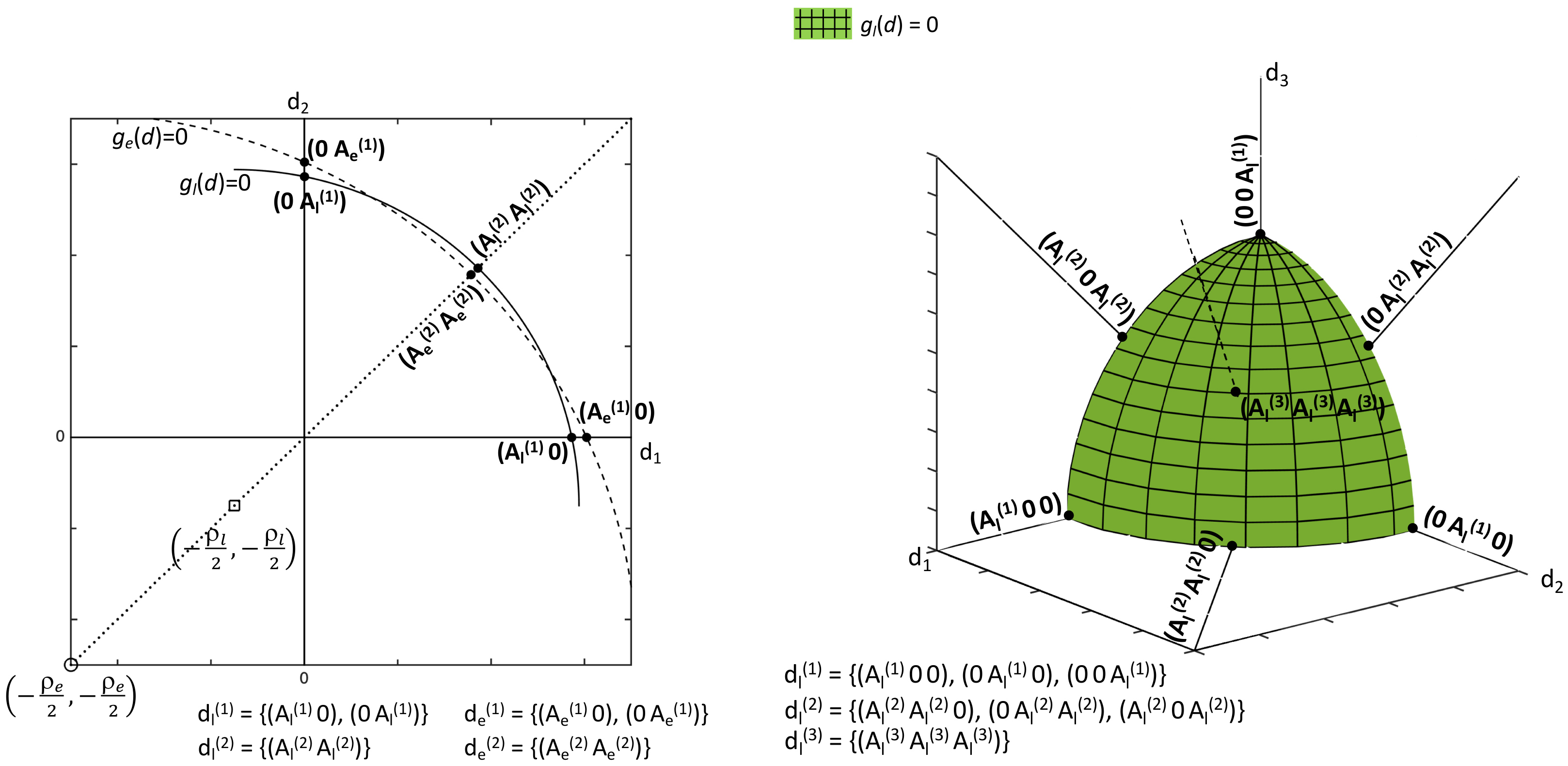
Theorem 2.

In the absence of the incomplete repair term, there are at most five different extremal candidates of Problem 1 given by the following representative structures:

$$\left(A^{\left(1\right)}0000\right),\left(A^{\left(2\right)}{A}^{\left(2\right)}000\right),\left(A^{\left(3\right)}{A}^{\left(3\right)}{A}^{\left(3\right)}00\right),\left(A^{\left(4\right)}{A}^{\left(4\right)}{A}^{\left(4\right)}{A}^{\left(4\right)}0\right),\left(A^{\left(5\right)}{A}^{\left(5\right)}{A}^{\left(5\right)}{A}^{\left(5\right)}{A}^{\left(5\right)}\right),$$

where

$$A^{\left(i\right)}=min\{A_e^{\left(i\right)},A_l^{\left(i\right)}\},i=1,\dots ,5,$$

(12)

and

$$A_e^{\left(i\right)}=-\frac{{\rho }_e}{2}+\sqrt{{\left(\frac{{\rho }_e}{2}\right)}^2+\frac{h_e}{i}},A_l^{\left(i\right)}=-\frac{{\rho }_l}{2}+\sqrt{{\left(\frac{{\rho }_l}{2}\right)}^2+\frac{h_l}{i}},i=1,\dots ,5.$$

(13)

Proof. 

A detailed proof of this result based on solving the Karush–Kuhn–Tucker system of necessary optimality conditions, is reported in [7]. In the present simpler, but practically meaningful, case of negligible interaction among dose fractions, a geometrical interpretation of the extremal solutions can be given and it is qualitatively illustrated by Figure 1 for $n=2$ and 3. It can be noticed that the expressions of the boundaries of Equations (8) and (9) represent hyperspheres with centers on the five-dimensional bisect line at $d_i=-{\rho }_e/2$, $d_i=-{\rho }_l/2$, for any i. Then, the problem extremals lie on the positive portions of the boundaries of $g_e\left(d\right)$, $g_l\left(d\right)$, and precisely of the most restrictive constraint boundary (see Equation (12)) as shown in the left panel of Figure 1. Increasing n, the set of candidates is enriched with additional structures, as illustrated in the right panel of Figure 1 for the simplified situation of a single prevalent quadratic constraint (for instance $g_l\left(d\right)$). The examples of Figure 1 can be considered representative of the more complex situation depicted by Theorem 1 (problem including dose interaction). Then, the problem geometry is similar to that of Figure 1 except for the fact that Equations (8)–(10) have elliptic contours, which makes the extremal set wider and the problem resolution more complicated. □

We remind that ${\rho }_e>{\rho }_l$ and we notice from Figure 1 that the admissibility of the structures of Theorem 2 depends on the relative position of the early and late constraint boundaries, i.e., on $h_e$ and $h_l$. Moreover, since the level surfaces of the cost function in Equation (10) are again hyperspheres with (fixed) center on the bisect line at $d_i=-\rho /2$, $i=1,\dots 5$, aligned with the early and late boundary centers, the optimum among the five structures depends on the value of $\rho$ with respect to ${\rho }_e$ and ${\rho }_l$. Denoting by $d_e^{\left(i\right)}$ and $d_l^{\left(i\right)}$, $i=1,\dots ,5$, the vectors with i non-zero entries equal to $A_e^{\left(i\right)}$ and $A_l^{\left(i\right)}$, respectively, we define the quantity

$$v=\frac{{(h_e-h_l)}^2}{({\rho }_e-{\rho }_l)({\rho }_e{h}_l-{\rho }_l{h}_e)},$$

(14)

which, as suggested by the geometrical interpretation of Figure 1, determines whether the early or instead the late constraint is prevalent. Here follows a sketch of the solutions for the simplified problem without incomplete repair term.

Theorem 3.

In the absence of the incomplete repair term, Problem 1 admits a unique optimal solution, apart from the previously mentioned equivalence of the structures in each class, when $\rho \ne {\rho }_l$ and $\rho \ne {\rho }_e$.

Table 2. Optimal solutions to Problem 1 for $\rho \ne {\rho }_l$ and $\rho \ne {\rho }_e$.

		$\mathit{\rho }<{\mathit{\rho }}_{\mathit{l}}$	${\mathit{\rho }}_{\mathit{l}}<\mathit{\rho }<{\mathit{\rho }}_{\mathit{e}}$	$\mathit{\rho }>{\mathit{\rho }}_{\mathit{e}}$
$h_e-h_l\le 0$		$d_e^{\left(1\right)}$	$d_e^{\left(1\right)}$	$d_e^{\left(5\right)}$
	$v\le 1$	$d_e^{\left(1\right)}$	$d_e^{\left(1\right)}$	$d_e^{\left(5\right)}$
$h_e-h_l>0$	$1<v<5$	$d_l^{\left(1\right)}$	$d_e^{\left(\right[v]+1)}$	$d_e^{\left(5\right)}$
	$v\ge 5$	$d_l^{\left(1\right)}$	$d_l^{\left(5\right)}$	$d_l^{\left(5\right)}$

reports the optimal solutions for $\rho \ne {\rho }_l$ and $\rho \ne {\rho }_e$, while

Table 3. Optimal solutions to Problem 1 for $\rho ={\rho }_l$ and $\rho ={\rho }_e$.

		$\mathit{\rho }={\mathit{\rho }}_{\mathit{l}}$	$\mathit{\rho }={\mathit{\rho }}_{\mathit{e}}$
$h_e-h_l\le 0$		$d_e^{\left(1\right)}$	$d_e^{\left(1\right)},d_e^{\left(2\right)},d_e^{\left(3\right)},d_e^{\left(4\right)},d_e^{\left(5\right)}$
	$v\le 1$	$d_e^{\left(1\right)}$	$d_e^{\left(1\right)},d_e^{\left(2\right)},d_e^{\left(3\right)},d_e^{\left(4\right)},d_e^{\left(5\right)}$
$h_e-h_l>0$	$1<v<5$	$d_l^{\left(1\right)},\dots ,d_l^{\left(\right[v\left]\right)}$	$d_e^{\left(\right[v]+1)},\dots ,d_e^{\left(5\right)}$
	$v\ge 5$	$d_l^{\left(1\right)},d_l^{\left(2\right)},d_l^{\left(3\right)},d_l^{\left(4\right)},d_l^{\left(5\right)}$	$d_l^{\left(5\right)}$

reports the optimal solutions for $\rho ={\rho }_l$ and $\rho ={\rho }_e$.

Proof. 

A rigorous proof is reported in [7] and it basically consists in expressing the cost function for any extremal point provided by Theorem 2 in terms of model parameters and in comparing its values. We remark that the result of this comparison depends on the value of $\rho$ with respect to ${\rho }_e$ and ${\rho }_l$. Reminding that the cost function level surfaces are concentric hyperspheres, the geometrical interpretation of the problem can give a hint on the optimal solution. Moreover, we note that, when v is an integer number between 1 and 5, then, for suitable $\rho$, the optimal solution is such that $d_e^{\left(v\right)}=d_l^{\left(v\right)}$, i.e., these vectors satisfy simultaneously the early and the late constraints with the equality sign. □

In Table 2 and Table 3, it emerges how the tumor radiosensitivity ratio $\rho$ determines the kind of optimal fractionation scheme. Indeed, hypofractionation is convenient for small $\rho$, whereas the optimal fractionation tends to be uniform for large $\rho$. This result formalizes in mathematical terms and confirms previous observations [32,33]. Other papers have then reported expressions of the optimal solution for similar problems in a form substantially equivalent to Equation (13) [11,34,35,36,37,38].

We consider now some applications that further specialize the previous results in terms of the important practical situation of prevalent late constraint.

Since the radiation-induced damages to healthy tissues cannot be directly measured, it is common to evaluate them as the damages produced by a reference radiotherapy protocol according to a chosen dose–response model [3,5]. Then, it is useful to introduce the Biologically Effective Dose (BED) defined as the total radiation dose proportional to the logarithmic cell kill that globally produces the same damage of a given protocol [39]. Using subscripts “e” and “l” as done previously, the maximal tolerable damages caused to normal tissue are expressed as $C_e={\alpha }_e{\mathrm{BED}}_e$ and $C_l={\alpha }_l{\mathrm{BED}}_l$. We set as the reference scheme, the conventional equi-fractionated scheme (one fraction/day, five fractions/week), with $\overline{n}$ fractions of size $\overline{d}$ over the time $\overline{T}$. Thus, we can write

$${\displaystyle C_e={\alpha }_e{\mathrm{BED}}_e=\overline{n}{\alpha }_e\overline{d}\left(1+\frac{\overline{d}}{{\rho }_e}\right)-\frac{ln\left(2\right)}{T_{Pe}}(\overline{T}-T_{Ke})H(\overline{T}-T_{Ke}),}$$

(15)

$$C_l={\alpha }_l{\mathrm{BED}}_l=\overline{n}{\alpha }_l\overline{d}\left(1+\frac{\overline{d}}{{\rho }_l}\right).$$

(16)

To simplify the comparisons of the numerical results for Problem 1 with data of real clinical protocols, we take as a reference protocol a radiotherapy scheme that includes an integer number of weeks, $\overline{\omega }$, with $\overline{n}=5\overline{\omega }$. From Equation (7), for the maximal weekly damages, we have

$$h_e={\rho }_{e}5\overline{d}\left(1+\frac{\overline{d}}{{\rho }_e}\right),h_l={\rho }_{l}5\overline{d}\left(1+\frac{\overline{d}}{{\rho }_l}\right).$$

(17)

From Equation (17), it is easy to verify that $h_e>h_l$, since ${\rho }_e>{\rho }_l$, and that $v=5$ (see Equation (14)). It has been shown in [7] (see Th. 6) that, for $h_e>h_l$, $v\ge 5$, the late constraint $g_l\left(d\right)$ dominates over $g_e\left(d\right)$ and the optimal solution is $d_l^{\left(1\right)}$ when $\rho <{\rho }_l$ or $d_l^{\left(5\right)}$ when $\rho >{\rho }_l$.

We performed numerical simulations to verify the previous results and compare them to the relevant literature. The normal tissue parameters, for which rather homogeneous estimates are available, were set to ${\rho }_l=3$ Gy, ${\rho }_e=10$ Gy, ${\alpha }_e=0.35$ Gy${}^{-1}$, $T_{ke}=7$ days, and $T_{pe}=2.5$ days [3,5]. To quantify $h_l$ and $h_e$, we considered a reference radiotherapy protocol and computed the damages it produces on normal tissues according to Equation (17). In particular, the “strong standard” fractionation schedule $35\mathrm{F}\times 2\mathrm{Gy}=70\mathrm{Gy}/46$ days ($\overline{\omega }=7$, $\overline{d}=2$ Gy) yields BED${}_l=116.7$ Gy and BED${}_e=53.1$ Gy [5,27].

Table 4. Numerical solutions to Problem 1 in the absence of incomplete repair for $\rho \in [1.5,20]$ Gy. $h_l=50.0$ Gy${}^2$, $h_e=120.0$ Gy${}^2$ computed by Equation (17) with $\overline{d}=2$ Gy. $\widehat{d}$: optimal solution; $\mathcal{D}$: optimal total dose.

		Optimal Values at $\widehat{\mathit{d}}$
$\mathit{\rho }$	Optimal Solution $\widehat{\mathit{d}}$	$\mathcal{D}$	$-\mathit{J}$	${\mathit{g}}_{\mathit{l}}$	${\mathit{g}}_{\mathit{e}}$
(Gy)	(Gy)	(Gy)		(Gy${}^{\mathbf{2}}$)	(Gy${}^{\mathbf{2}}$)
$[1.5,3)$	$\left(5.72840000\right)$	$5.7284$	$[41.407,50.000)$	0	$-29.901$
3	$\left(5.72840000\right)$	$5.7284$	$50.000$	0	$-29.901$
	$\left(3.72023.7202000\right)$	$7.4403$			$-17.918$
	$\left(2.84932.84932.849300\right)$	$8.5480$			$-10.164$
	$\left(2.34062.34062.34062.34060\right)$	$9.3623$			$-4.464$
	$\left(2.00002.00002.00002.00002.0000\right)$	$10.0000$			0
$(3,20]$	$\left(2.00002.00002.00002.00002.0000\right)$	$10.0000$	$(50.000,220.000]$	0	0

reports the optimal solutions as $\rho$ changes in a meaningful value range. For a comparison with the literature,

Table 5. Comparison of LCK, BED${}_l$ and BED${}_e$ between the reference protocol ($\overline{\omega }=7$, $\overline{d}=2$ Gy) and the optimal solution to Problem 1 in the absence of incomplete repair. Parameters: $\rho =1.5$ Gy, $\alpha =0.1$ Gy${}^{-1}$, $T_P=40$ days, and $T_k=300$ days; $\rho =10$ Gy, $\alpha =0.35$ Gy${}^{-1}$, $T_P=3$ days, and $T_k=21$ days.

		Optimal Values at $\widehat{\mathit{d}}$			Reference Protocol Values
$\mathit{\rho }$	Optimal Solution $\widehat{\mathit{d}}$	LCK	BED${}_{\mathit{l}}$	BED${}_{\mathit{e}}$	LCK	BED${}_{\mathit{l}}$	BED${}_{\mathit{e}}$
(Gy)			(Gy)	(Gy)		(Gy)	(Gy)
$1.5$	$\left(5.72840000\right)$	$8.392$	$116.667$	$32.175$	$7.093$	$116.667$	$53.105$
10	$\left(2.00002.00002.00002.00002.0000\right)$	$10.260$	$116.667$	$53.105$	$10.260$	$116.667$	$53.105$

focuses on $\rho =1.5$ Gy and $\rho =10$ Gy, typically associated to slowly proliferating tumors (prostate) and fast proliferating tumors (head and neck, lung).

Table 5 includes the computation of a quantity often used to evaluate the treatment efficacy, i.e., the tumor “log cell kill” (LCK) defined by $\mathrm{LCK}={\log }_{10}(1/S)$ and given by

$$\mathrm{LCK}={\log }_{10}\left(\mathrm{e}\right)\left(E_1+E_2-E_3\right),$$

(18)

with S as in Equation (4) and $E_2=0$, $E_1$, and $E_3$ as in Equations (1) and (3). As expected, for $\rho =10$ Gy, the optimal solution coincides with the corresponding reference protocol. Conversely, when $\rho =1.5$ Gy, the optimal solution is not uniform and it consists of a single fractional dose of amplitude higher than the conventional (reference) value. Thus, in agreement with several literature results, we find that, when $\rho <{\rho }_l$, the optimum is given by hypo-fractionated protocols (see, e.g., [5,28,32,33]).

A remark can be made about the normal tissue constraints considered in the present study. In the problem formulation, only two kinds of healthy tissue reactions, early and late, were taken into account. Moreover, the radiation response of tissues is considered homogeneous disregarding the spatial or inter-individual differences. Although simplistic, this representation of surrounding organs at risk is thought to capture the essential aspects in the optimization of traditional radiotherapy schedules and it actually is most commonly considered in the literature. However, expressing the damages as in Equations (1)–(5), we assumed that the normal tissues receive the same amount of radiation, i.e., the same fraction doses $d_i$, of the tumor, which is not very realistic. Indeed, modern techniques make increasingly feasible to deliver high fractions to the tumor while reducing the fractions to the surrounding tissues by spatially modulating the radiation intensity. While modeling such remarkable aspects is beyond the scope of the present work, it can be interesting to give an idea of some resulting effects on the optimal solutions. In [7], this was done by introducing a global coefficient, $f\in (0,1)$, to represent, on average, the attenuation of the dose received by normal tissues with respect to the tumor. Then, the effective fractional doses acting on normal tissues are $f{d}_i,i=1,\dots ,5$, in the related constraint expressions, i.e., in all the damage terms of Equation (5), or $f\overline{d}$ in the expressions of $C_e$, $C_l$ computed by the reference protocol as in Equations (15) and (16). Moreover, to get expressions of $g_e\left(d\right)$, $g_l\left(d\right)$ of the kind in Equations (8) and (9), we have to redefine accordingly the notation related to the normal tissue parameters (see also [7]). In particular, we upgrade the notation in Equation (7) setting

$${\rho }_e=\frac{{\alpha }_e}{f{\beta }_e},{\rho }_l=\frac{{\alpha }_l}{f{\beta }_l},h_e=\frac{C_e+E_{3e}}{f^2\omega {\beta }_e},h_l=\frac{C_l}{f^2\omega {\beta }_l}.$$

(19)

The optimal solutions of Problem 1 computed with $f=0.3$ are reported in

Table 6. Numerical solutions to Problem 1 in the absence of incomplete repair. Actual dose to normal tissue reduced by a factor $f=0.3$, resulting in $h_l=120.0$ Gy${}^2$ and $h_e=353.3$ Gy${}^2$. Optimal solutions for $\rho \in [1.5,50]$ Gy. $\widehat{d}$, optimal solution; $\mathcal{D}$, optimal total dose.

		Optimal Values at $\widehat{\mathit{d}}$
$\mathit{\rho }$	Optimal Solution $\widehat{\mathit{d}}$	$\mathcal{D}$	$-\mathit{J}$	${\mathit{g}}_{\mathit{l}}$	${\mathit{g}}_{\mathit{e}}$
(Gy)	(Gy)	(Gy)		(Gy${}^{\mathbf{2}}$)	(Gy${}^{\mathbf{2}}$)
$[1.5,10)$	$\left(7.04160000\right)$	$7.0416$	$[60.146,120.000)$	0	$-69.030$
10	$\left(7.04160000\right)$	$7.0416$	$120.000$	0	$-69.030$
	$\left(4.21954.2195000\right)$	$8.4391$			$-36.421$
	$\left(3.06233.06233.062300\right)$	$9.1868$			$-18.975$
	$\left(2.41622.41622.41622.41620\right)$	$9.6648$			$-7.822$
	$\left(2.00002.00002.00002.00002.0000\right)$	$10.0000$			0
$(10,50]$	$\left(2.00002.00002.00002.00002.0000\right)$	$10.0000$	$(120.000,520.000]$	0	0

for a comparison with the results of Table 4 where $f=1$. In the simulation of Table 6, the reference fraction dose $\overline{d}=2$ Gy is left unchanged, but the maximal damages $C_e$ and $C_l$ are computed from Equations (15) and (16) using $f\overline{d}$ instead of $\overline{d}$. Then, the limits $h_e$, $h_l$ are evaluated from Equation (19) obtaining expressions formally identical to Equation (17), provided that the parameters ${\rho }_e$, ${\rho }_l$ are given as in Equation (19).

The optimal solutions are found to be structurally identical to those of Table 4, but the solution pattern appears to be shifted towards higher $\rho$ values (so allowing hypofractionation also for tumors with relatively high $\rho$, $\rho <10$ Gy in the example), while larger optimal doses are permitted in hypofractionated schemes.

4. Introduction of an Upper Bound on the Daily Fractional Dose

A single fraction dose per week was found to be optimal for slowly proliferating tumors, either taking into account the sublethal damage due to incomplete repair or not [7]. Then, if the maximal tolerable damages to normal tissues are computed on the basis of the conventional uniform protocols, the dose fraction sizes can become as large as to make the theoretical optimal solution practically unacceptable. We remind that the direct evaluation of the maximal admissible radiation damage is obviously impossible, so that the method usually applied is the one using clinically assessed reference protocols, as described by Equation (17).

In the paper [8], we reconsidered the optimization problem (Problem 1) in the absence of a sublethal damage term owing to incomplete repair and over a fixed treatment time, and we introduced a linear constraint representing an upper bound for the daily fractional dose. The additional constraint is included to strengthen the normal tissue constraints, particularly with respect to “late” collateral complications occurring months or even years after the radiation treatment. As already mentioned, the quantification of this kind of complications by means of the LQ model is a controversial issue, especially at high fraction doses [5,16,17,18,19,40,41].

Despite the formulation simplicity, including such box constraints on the fractional doses makes the solution of the problem rather complex. In this section, we summarize the analytical results reported by Bruni et al. [8], postponing a more detailed description of the solution until the next section where the optimization problem is solved also with respect to the treatment duration.

As done for Problem 1, we assume that the overall treatment time is fixed and given by $T=7\omega -3$, and that the cumulative damages to normal tissues are equi-distributed over the $\omega$ treatment weeks. Then, we formulate the following optimization problem over a single week of treatment, where $d_M$ denotes the maximal value of the daily fraction and $g_e\left(d\right),g_l\left(d\right)$ are defined by Equations (8) and (9), without the incomplete repair term.

Problem 2.

Minimize the function:

$$J\left(d\right)=-\rho \sum _{i=1}^5{d}_i-\sum _{i=1}^5{d}_i^2,$$

(20)

on the admissible set:

$$D=\{d\in {\mathbb{R}}^5|d_i\in [0,d_M],i=1,\dots ,5,g_e\left(d\right)\le 0,g_l\left(d\right)\le 0\}.$$

A complete picture of the optimal solutions to Problem 2 is given in [8], where the dependence of the optimum on the tumor $\alpha /\beta$ and on the bound $d_M$ is investigated. Incidentally, we observe that the problem considered in the present section is actually a particular case of the problem considered in Section 5 when $n=5$.

Here, we report only the optimal solutions for the situation of prevalent late constraint most frequently considered in practical applications (see

Table 7. Optimal solutions to Problem 2 with respect to the tumor parameter $\rho$ and the value of $d_M$ for prevalent late constraint.

${\mathit{d}}_{\mathit{M}}$	$\left({\mathit{A}}_{\mathit{l}}(\mathit{u}+\mathbf{1},\mathbf{0}),{\mathit{A}}_{\mathit{l}}(\mathit{u},\mathbf{0})\right]$	$\left({\mathit{A}}_{\mathit{l}}(\mathbf{1},\mathbf{0}),\infty \right)$
	$\mathbf{1}\le \mathit{u}\le \mathbf{4}$
$\rho <{\rho }_l$	$d_l(1,u)$	$d_l(1,0)$
$\rho \ge {\rho }_l$	$d_l(5,0)$	$d_l(5,0)$

). In Table 7, the quantities $d_l(i,j)$ are solutions of $g_l\left(d\right)=0$ having j entries equal to $d_M$, i entries equal to $A_l(i,j)$ and, clearly, $5-i-j$ null entries. For suitable $i,j$, the value $A_l(i,j)$ is defined as

$$A_l(i,j)=-\frac{{\rho }_l}{2}+\sqrt{{\left(\frac{{\rho }_l}{2}\right)}^2+\frac{h_l-j{d}_M(d_M+{\rho }_l)}{i}}.$$

(21)

Figure 2 illustrates the behavior of the fractional doses of the optima in Table 7 for $\rho <{\rho }_l$, showing how they change as a function of $d_M$.

5. Optimal Number and Sizes of the Fractional Doses

In the present section we introduce the interesting aspect of finding the optimum overall treatment time. Using the same formalism of the previous sections, we extend the formulation of Problem 2 to an arbitrary number n of dose fractions, thus removing the assumption of treatments administered over an assigned integer number of weeks. As done above, we consider traditional EBRT schemes with one fraction per day and treatment breaks at the weekends and we express the overall treatment duration $T=T\left(n\right)$ as

$$T\left(n\right)=7\left[\frac{n}{5}\right]-1-\left\{\begin{array}{cc}2,\hfill & \mathrm{n}/5\mathrm{integer},\hfill \\ 5\left[\frac{n}{5}\right]-n,\hfill & \mathrm{else}.\hfill \end{array}\right.$$

(22)

Fixing a relation between the number of dose fractions and the overall treatment time allows us to consider the number and the sizes of the dose fractions as the only decision variables. Obviously, the choice in Equation (22) is non-restrictive since different expressions of $T\left(n\right)$ could be envisaged without substantially altering the problem solving procedure (e.g., two fractions/day or seven fractions/week). Numerical examples with different irradiation schemes investigating how clinically important factors, such as accelerated tumor repopulation, affect the optima are reported in [9]. Then, the problem studied here is that of minimizing the function $\ln \left(S\right)$ (with S given by Equation (4)) with respect to both number and sizes of the fractional doses, taking into account the constraints on the normal tissue damages in Equation (5) (without incomplete repair) and the upper bound $d_M$ on the fractional dose sizes.

Using the usual notation in Equation (7), the total maximal admissible damages $k_e\left(n\right)$, $k_l$ over the time $T\left(n\right)$ are

$$k_e\left(n\right)=\frac{1}{{\beta }_e}\left[C_e+\frac{ln\left(2\right)}{T_{Pe}}\left(T\left(n\right)-T_{Ke}\right)H\left(T\left(n\right)-T_{Ke}\right)\right],k_l=\frac{C_l}{{\beta }_l}.$$

(23)

The following optimization problem can be set in terms of the variables n (number of fractional doses) and d (vector of the fractional dose sizes $d_i$, with $i=1,\dots ,n$).

Problem 3.

Minimize the function:

$$J(n,d)=-\rho \sum _{i=1}^n{d}_i-\sum _{i=1}^n{d}_i^2+\frac{ln\left(2\right)}{\beta T_P}\left(T\left(n\right)-T_K\right)H\left(T\left(n\right)-T_K\right),$$

(24)

on the admissible domain:

$$D=N\times D_n$$

(25)

where

$$\begin{gathered} N=\{n\in \mathbb{N}|1\le n\le n_M\}, \\ {D}_n=\{d\in {\mathbb{R}}^n\hspace{1em}|\hspace{1em}{g}_e(n,d)={\rho }_e\sum _{i=1}^n{d}_i+\sum _{i=1}^n{d}_i^2-k_e\left(n\right)\le 0, \\ {g}_l(n,d)={\rho }_l\sum _{i=1}^n{d}_i+\sum _{i=1}^n{d}_i^2-k_l\le 0, \end{gathered}$$

(26)

$$\begin{array}{c}0\le d_i\le d_M,i=1,\dots ,n\}.\hfill \end{array}$$

(27)

5.1. Optimal Vectors d

Problem 3 can be decomposed into a finite collection of $n_M$ optimization subproblems to be solved in cascade with respect to $d\in D_n$, for n fixed, and then with respect to n, for any $n\in N$. In fact, recalling Equations (25)–(27) of the feasible set D, we can write

$$\underset{(n,d)\in D}{min}J(n,d)=\underset{n\in N}{min}\left(\underset{d\in D_n}{min}J(n,d)\right).$$

(28)

Moreover

$$J(n,d)=J_n\left(d\right)+E\left(n\right),$$

(29)

where

$$J_n\left(d\right)=-\rho \sum _{i=1}^n{d}_i-\sum _{i=1}^n{d}_i^2,$$

(30)

and

$$E\left(n\right)=\frac{ln\left(2\right)}{\beta T_P}\left(T\left(n\right)-T_K\right)H\left(T\left(n\right)-T_K\right).$$

(31)

Since $E\left(n\right)$ in Equation (31) does not depend on the doses, the problem of minimizing $J(n,d)$ on $D_n$ is equivalent to that of minimizing $J_n\left(d\right)$ on the same set when n is fixed. Thus, we start by the minimization with respect to d alone, i.e., by solving the following problem, which is a rather direct extension of Problem 2.

Problem 4.

For any fixed $n\in N$, minimize the function $J_n\left(d\right)$ in Equation (30) with respect to d on the admissible set $D_n$ in Equation (27).

The decomposition in Equation (28) evidences that, in view of the Weierstrass Theorem [31], the compactness of $D_n$ and the continuity of $J_n\left(d\right)$ on $D_n$ guarantee the existence of an optimal solution for Problem 4 for any given $n\in N$. Let us denote by $d_n^{\star }$ such an optimal solution, defining the sequence of the corresponding optimal values for $n\in N$

$$J^{\star }\left(n\right)=J(n,d_n^{\star })=\underset{d\in D_n}{min}J(n,d).$$

(32)

Since N is of finite cardinality, the optimum of Problem 3 can be determined by performing a finite number of direct comparisons among the values $J^{\star }\left(n\right)$, $n\in N$.

The optimal solutions of Problem 4 for an arbitrary $n\in [1,n_M]$ have been derived in [9] solving the Karush–Kuhn–Tucker necessary and admissibility system, in view of the existence property guaranteed by the Weierstrass theorem [31]. Because of the problem structure where the cost function and the constraints are symmetrical with respect to the n-dimensional line $\ell =\{d\in {\mathbb{R}}^n:d_i=d_{i+1},i=1,\dots ,n-1\}$, the necessary and admissibility conditions increase with n, while their structure is unchanged. In view of its application by numerical simulation, we report here the conclusive theorem of Bruni et al. [9] for the most general constraint geometry.

Theorem 4.

For $k_e\left(n\right)-k_l>0$, ${\rho }_e{k}_l-{\rho }_l{k}_e\left(n\right)>0$, and $1\le v\le n$, the optimal solutions of Problem 4 in terms of ρ and $d_M$ are as in

Table 8. Optimal solutions $d_n^{\star }$ with respect to $\rho$ and $d_M$ for $1<v<n$. The column headings reporting additional conditions on v indicate that the solutions exist only for the values specified. The vectors for ${\rho }_l\le \rho <{\rho }_e$, $d_M\ge R_{1\left[v\right]}$, and $\rho ={\rho }_e$ are representative optimal vectors.

${\mathit{d}}_{\mathit{M}}$	$\left(\mathbf{0},{\mathit{A}}_{\mathit{e}}(\mathit{n},\mathbf{0})\right)$	$\left[{\mathit{A}}_{\mathit{e}}(\mathit{u}+\mathit{1},\mathbf{0}),{\mathit{A}}_{\mathit{e}}(\mathit{u},\mathbf{0})\right)$	$\left[{\mathit{A}}_{\mathit{e}}(\left[\mathit{v}\right]+\mathbf{1},\mathbf{0}),{\mathit{R}}_{\mathbf{1}\left[\mathit{v}\right]}\right)$	${\mathit{R}}_{\mathbf{1}\left[\mathit{v}\right]}$	$\left({\mathit{R}}_{\mathbf{1}\left[\mathit{v}\right]},{\mathit{A}}_{\mathit{l}}(\left[\mathit{v}\right],\mathbf{0})\right]$	$\left({\mathit{A}}_{\mathit{l}}(\mathit{u}+\mathit{1},\mathbf{0}),{\mathit{A}}_{\mathit{l}}(\mathit{u},\mathbf{0})\right]$	$\left({\mathit{A}}_{\mathit{l}}(\mathbf{1},\mathbf{0}),\infty \right)$
		$\left[\mathit{v}\right]+\mathit{1}\le \mathit{u}\le \mathit{n}-\mathit{1}$				$\mathbf{1}\le \mathit{u}\le \left[\mathit{v}\right]-\mathbf{1}$
$\mathit{v}$	-	$<\mathit{n}-\mathbf{1}$	-	-	$\ne \left[\mathit{v}\right]$	$>\mathbf{2}$	-
$\rho <{\rho }_l$	$\tilde{d}$	$d_e(1,u)$	$d_e(1,\left[v\right])$	$d^R$	$d_l(1,\left[v\right])$	$d_l(1,u)$	$d_l(1,0)$
$\rho ={\rho }_l$	$\tilde{d}$	$d_e(1,u)$	$d_e(1,\left[v\right])$	$d^R$	$d^R$	$d^R$	$d^R$
${\rho }_l<\rho <{\rho }_e$	$\tilde{d}$	$d_e(1,u)$	$d_e(1,\left[v\right])$	$d^R$	$d^R$	$d^R$	$d^R$
$\rho ={\rho }_e$	$\tilde{d}$	$d_e(n,0)$	$d_e(n,0)$	$d_e(n,0)$	$d_e(n,0)$	$d_e(n,0)$	$d_e(n,0)$
$\rho >{\rho }_e$	$\tilde{d}$	$d_e(n,0)$	$d_e(n,0)$	$d_e(n,0)$	$d_e(n,0)$	$d_e(n,0)$	$d_e(n,0)$

,

Table 9. Optimal solutions $d_n^{\star }$ with respect to $\rho$ and $d_M$ for $v=1$. The vectors for $\rho ={\rho }_e$ are representative optimal vectors.

${\mathit{d}}_{\mathit{M}}$	$\left(\mathbf{0},{\mathit{A}}_{\mathit{e}}(\mathit{n},\mathbf{0})\right)$	$\left[{\mathit{A}}_{\mathit{e}}(\mathit{u}+\mathbf{1},\mathbf{0}),{\mathit{A}}_{\mathit{e}}(\mathit{u},\mathbf{0})\right)$	$\left[{\mathit{A}}_{\mathit{e}}(\mathbf{1},\mathbf{0}),\infty \right)$
		$\mathbf{1}\le \mathit{u}\le \mathit{n}-\mathbf{1}$
$\rho <{\rho }_e$	$\tilde{d}$	$d_e(1,u)$	$d_e(1,0)$
$\rho ={\rho }_e$	$\tilde{d}$	$d_e(n,0)$	$d_e(n,0)$
$\rho >{\rho }_e$	$\tilde{d}$	$d_e(n,0)$	$d_e(n,0)$

and

Table 10. Optimal solutions $d_n^{\star }$ with respect to $\rho$ and $d_M$ for $v=n$. The vectors for $\rho ={\rho }_l$ are representative optimal vectors.

${\mathit{d}}_{\mathit{M}}$	$\left(\mathbf{0},{\mathit{A}}_{\mathit{l}}(\mathit{n},\mathbf{0})\right)$	$\left[{\mathit{A}}_{\mathit{l}}(\mathit{u}+\mathbf{1},\mathbf{0}),{\mathit{A}}_{\mathit{l}}(\mathit{u},\mathbf{0})\right)$	$\left[{\mathit{A}}_{\mathit{l}}(\mathbf{1},\mathbf{0}),\infty \right)$
		$\mathbf{1}\le \mathit{u}\le \mathit{n}-\mathbf{1}$
$\rho <{\rho }_l$	$\tilde{d}$	$d_l(1,u)$	$d_l(1,0)$
$\rho ={\rho }_l$	$\tilde{d}$	$d_l(n,0)$	$d_l(n,0)$
$\rho >{\rho }_l$	$\tilde{d}$	$d_l(n,0)$	$d_l(n,0)$

.

Proof. 

A proof of Theorem 4 is reported in the paper [9] along with a detailed analysis of the results. We remind that, in Table 8, $d_e(i,j)$ denotes solutions of $g_e(n,d)=0$ having j entries equal to $d_M$, i entries equal to $A_e(i,j)$, and the remaining $n-i-j$ entries equal to zero. $A_e(i,j)$ is defined by

$$A_e(i,j)=-\frac{{\rho }_e}{2}+\sqrt{{\left(\frac{{\rho }_e}{2}\right)}^2+\frac{k_e\left(n\right)-j{d}_M(d_M+{\rho }_e)}{i}}.$$

(33)

Similarly, we can define $d_l(i,j)$ and $A_l(i,j)$, with

$$A_l(i,j)=-\frac{{\rho }_l}{2}+\sqrt{{\left(\frac{{\rho }_l}{2}\right)}^2+\frac{k_l-j{d}_M(d_M+{\rho }_l)}{i}}.$$

(34)

It is evident in Table 8 that the optimal framework of Problem 4 becomes rather complex, especially in the absence of a prevalent constraint. The optimal solution now changes as the pair of model parameters ($\rho$ and $d_M$) change, as well as when the geometry of the normal tissue constraint is modified (which means changing v). Figure 3 depicts such diversified situation reporting two three-dimensional examples of the optima for the case of a slowly proliferating tumor ($\rho <{\rho }_l$) and for two $d_M$ values: higher $d_M$ ($d_M>A_l(1,0)$, left panel) and lower $d_M$ ($A_l(2,0)<d_M<A_l(1,0)$, right panel).

In [8,9], it is shown that, when $\rho <{\rho }_l$, the cost function evaluated for $d_l(i,j)$ and $d_e(i,j)$ decreases as the total dose of the solution decreases. Thus, among the admissible vectors, the optimum is given by the one with the minimal total dose. Indeed, when $d_M>A_l(1,0)$, $d_l(1,0)$ is the optimum (first row, last column of Table 8) since it is admissible (Figure 3, left panel) and since it satisfies the minimal total dose requirement. On the contrary, when $d_M<A_l(1,0)$, the solution $d_l(1,0)$ is no longer admissible as it violates the box constraint (Figure 3, right panel). Thus, provided that $d_M\ge A_l(2,0)$, the new selected optimum is $d_l(1,1)$ (first row, second to last column of Table 8, with $u=1$), which is again the vector with the minimal total dose among all the admissible vectors. □

Concerning Table 8, we observe that there exists a threshold value for $d_M$, which is called $R_{1\left[v\right]}$, discriminating whether points of the intersection set $\{d\in {\mathbb{R}}^n:g_e(n,d)=0,g_l(n,d)=0\}$ are admissible or not. In fact, such points are admissible if and only if $d_M\ge R_{1\left[v\right]}$. Then, depending on $d_M$ and v, the optimal solution can belong to the mentioned intersection of the constraints. As a representative vector of this set, we choose the vector, denoted by $d^R$, with the following particular structure: $\left[v\right]$ components equal to $R_{1\left[v\right]}$, one component equal to $S-\left[v\right]R_{1\left[v\right]}$ (absent for $v=n$), plus $n-\left[v\right]-1$ components equal to zero (absent if $v\ge n-1$). Our computational results show that $d^R$ can actually represent the optimal radiotherapy scheme for tumors with $\rho$ intermediate between ${\rho }_l$ and ${\rho }_e$.

5.2. Optimal n

Let us now consider the function $J^{\star }\left(n\right)$, defined by Equation (32), as $J(n,d)$ evaluated at the optimum $d_n^{\star }$ of Problem 4, with $J(n,d)$ in Equations (29)–(31). We have

$${\displaystyle J^{\star }\left(n\right)=J_n\left(d_n^{\star }\right)+E\left(n\right).}$$

(35)

Concerning the problem of minimizing $J^{\star }\left(n\right)$ with respect to n, in the paper [9], we established a result that yields a theoretical upper limit for the optimal number of fractions and then for the optimal treatment time. Therefore, provided that $n_M$ is higher than the upper limit, the iterative searching procedure surely terminates in a finite number of steps leading to the optimal fraction number $n^{\circ }$, $n^{\circ }\in [1,n_M]$. The theoretical upper bound depends on whether the tumor $\rho$ is smaller or greater than ${\rho }_l$, as stated in the following theorem.

Theorem 5.

For $n\ge 1$, the value $n^{\circ }$ for which $J^{\star }\left(n\right)$ defined in Equation (35) attains its minimum value exists and it is finite. For $\rho <{\rho }_l$, it is $n^{\circ }\le a$, where a is such that ${\rho }_e{k}_l-{\rho }_l{k}_e\left(a\right)=0$. For $\rho \ge {\rho }_l$, in the presence of tumor repopulation starting at $T_K$, it is $n^{\circ }<\tilde{n}$, where $\tilde{n}$ is defined by

$$\tilde{n}=\frac{1}{ln\left(2\right)}\frac{\alpha k_l}{{\rho }_l}\frac{T_P}{\Delta }+\frac{T_K}{\Delta }+1$$

(36)

Proof. 

(see [9] for the details). Clearly, the thesis stems from the behavior of $J^{\star }\left(n\right)$ and, in particular, from the balance of its composing terms with respect to n. In addition, the conclusion depends on $\rho$ being smaller or greater than ${\rho }_l$ because of the optimality of different fractionation schemes (see Table 8, Table 9 and Table 10). Then, under the stated assumptions, it is easy to verify some properties of the functions $J_n\left(d_n^{\star }\right)$ and $E\left(n\right)$ useful to get the conclusion: (1) $J_{n+1}\left(d_{n+1}^{\star }\right)\le J_n\left(d_n^{\star }\right)<0$; (2) $J_n\left(d_n^{\star }\right)$ has a finite (negative) lower bound; (3) $E(n+1)\ge E\left(n\right)\ge 0$; and (4) $E\left(n\right)\ge ln\left(2\right)((n-1)\Delta -T_K)/\left(\beta T_P\right)$, $\Delta =1$ day.

Another property stated in [9] is that, for $n\ge a$, with a defined in theorem statement, $g_l(n,d)$ is stricter than $g_e(n,d)$, which means that for n increasing the optimal vector eventually belongs to the boundary of the late constraint. Then, for $n\ge a$, the optimum is $d_n^{\star }=d_l(1,u)$ for $\rho <{\rho }_l$ and $d_n^{\star }=d_l(n,0)$ for $\rho \ge {\rho }_l$ (see Table 10).

For $\rho <{\rho }_l$, the integer u in the optimum $d_n^{\star }=d_l(1,u)$ is independent of n (but it depends on $d_M$). Hence, $J_n\left(d_n^{\star }\right)$ takes a constant value with respect to n for $n\ge a$ and this constant value constitutes its minimum. Thus, according to Properties (1)–(4), it is $n^{\circ }\le a$ (independently of the possible tumor repopulation).

For $\rho \ge {\rho }_l$, substituting the optimum $d_n^{\star }=d_l(n,0)$ in the cost function, and reminding Equation (34) of $A_l(n,0)$, it can be proved that $J_n\left(d_n^{\star }\right)$ strictly decreases with n tending to the finite negative limit $-\rho k_l/{\rho }_l$. The presence of tumor repopulation will contrast the descent of $J_n\left(d_n^{\star }\right)$ for n increasing. Using Property (4), we can write

$$J^{\star }\left(n\right)>-\frac{\rho k_l}{{\rho }_l}+\frac{ln\left(2\right)}{\beta T_P}[(n-1)\Delta -T_K],$$

(37)

where the right hand side is increasing with n. Denoting by $\tilde{n}$ the real value where the minorant in Equation (37) vanishes, we get for $\tilde{n}$ the finite value defined in Equation (36). In conclusion, $J^{\star }\left(n\right)$ is negative and non-increasing until $T\left(n\right)\le T_K$ and it is positive for $n\ge \tilde{n}$. Therefore, $J^{\star }\left(n\right)$ must attain its minimum for $n^{\circ }<\tilde{n}$. □

6. Numerical Results

We report a concise review of the main numerical results on the optimal solution of Problem 3. We concentrate on this latter problem because the results allow us to evidence also properties common to the solution of Problems 1 and 2.

On the basis of the analytical results of Section 5.1, after setting $n_M$, the numerical procedure selects the optimal solution $d_n^{\star }$ for each $n=1,\dots ,n_M$ computing the related $J(n,d_n^{\star })=J^{\star }\left(n\right)$. Then, the optimal fraction number $n^{\circ }$ is the number for which $J^{\star }\left(n\right)$ attains its minimum value. Moreover, still according to the theoretical results of the previous sections, our numerical investigation focuses on three tumor classes, each identified by an interval of radiosensitivity ratio values: high ($\rho \ge {\rho }_e$, fast proliferating tumors), low ($\rho <{\rho }_l$, slowly proliferating tumors), and intermediate (${\rho }_l\le \rho <{\rho }_e$).

As mentioned above, the classification of tumors based on their proliferative behavior and on $\alpha /\beta$ estimates has been widely used in the literature, while the advantage of using different non-conventional protocols for different tumor classes has been evidenced only recently. Therefore, our simulations were organized to explore the effect on the optimum of changing the tumor parameters.

For the computation of the maximal admissible damages $C_e$ and $C_l$, again we chose an equi-fractionated reference protocol $\overline{n}\mathrm{F}\times \overline{d}\mathrm{Gy}/\overline{T}\mathrm{days}$, of the kind one fraction/day, five fractions/week. From Equations (15) and (23), we obtain

$$k_e\left(n\right)={\overline{k}}_e+\frac{ln\left(2\right)}{{\beta }_e{T}_{Pe}}\left(T\left(n\right)-T_{Ke}\right)H\left(T\left(n\right)-T_{Ke}\right),$$

(38)

where the term ${\overline{k}}_e$ is independent of n and entirely attributable to the reference protocol

$${\overline{k}}_e=\overline{n}{\rho }_e\overline{d}\left(1+\frac{\overline{d}}{{\rho }_e}\right)-\frac{ln\left(2\right)}{{\beta }_e{T}_{Pe}}\left(\overline{T}-T_{Ke}\right)H\left(\overline{T}-T_{Ke}\right).$$

From Equation (16), we have

$$k_l=\overline{n}{\rho }_l\overline{d}\left(1+\frac{\overline{d}}{{\rho }_l}\right).$$

(39)

The simulations were carried out setting $d_M$ so that it satisfies the reasonable condition $\overline{d}\le d_M<min\{{\overline{A}}_e(1,0),A_l(1,0)\}$, where $\overline{d}$ is the fractional dose of the reference protocol and ${\overline{A}}_e(1,0)$ is computed setting $k_e\left(n\right)={\overline{k}}_e$ and $(i,j)=(1,0)$ in Equation (33). The above condition ensures optimal treatments consisting of at least two fractions besides the admissibility of the reference protocol.

The values of the normal tissue parameters are relatively well assessed in the literature, whereas the tumor parameter estimates vary considerably, even for the same tumor type. A rather detailed literature search led us to fix in all the simulations the parameters of early and late normal tissue as ${\rho }_e=10$ Gy, ${\alpha }_e=0.35$ Gy${}^{-1}$, and $T_{Ke}=7$ days and $T_{Pe}=2.5$ days, and ${\rho }_l=3$ Gy, respectively [3,4,5,42].

Concerning the tumor classes, fast proliferating tumors characterized by high radiosensitivity ratios are reckoned to include most human tumors, for instance head and neck, lung, and cervical cancers [4,27,29,30,43]. We identify this tumor type with the range $\rho \ge {\rho }_e$. Currently, prostatic cancers are known as the most slowly proliferating human tumors; such tumors exhibit long potential doubling times, low proportions of cycling cells, and low radiosensitivity ratios, typically lower than late-responding normal tissues ($\rho <{\rho }_l$) [32,33,44,45,46,47,48,49]. Examples of tumors with ${\rho }_l\le \rho <{\rho }_e$ are breast cancer and some prostatic cancers observed to be not assimilable to slowly proliferating tumors [30,50,51].

In view of the large variability of tumor parameters, we assumed a nominal set of parameter values for each tumor class, and then we explored how the optimal solution changes when the parameters vary in a meaningful range of values. Indeed, this is a crucial point for the application of our optimization procedure because it requires setting the values of parameters such as $\rho$ and $\alpha$, which can be affected by considerable estimation errors [21,35]. Interestingly, our simulations showed some robustness of the optimal protocols to variations of the parameters, as shown below.

We are interested in comparing the obtained optimal protocols to real clinical schedules, which can be done evaluating by means of the LQ model the effects that they produce in terms of cell killing. As in Section 1, we chose the commonly used “strong standard” reference protocol $35\mathrm{F}\times 2\mathrm{Gy}=70\mathrm{Gy}/46$ days, which provides BED${}_l=116.7$ Gy, BED${}_e=53.1$ Gy [5,27] and consequently $k_l=350$ Gy${}^2$, ${\overline{k}}_e=C_e/{\beta }_e=531.05$ Gy${}^2$. The “log cell kill” defined in Equation (18) to quantify tumor radiation damages now takes the form

$$\mathrm{LCK}=\alpha {log}_{10}\left(\mathrm{e}\right)\left[{\displaystyle \sum _{i=1}^n{d}_i+\frac{1}{\rho }\sum _{i=1}^n{d}_i^2-\frac{ln\left(2\right)}{\alpha T_P}(T\left(n\right)-T_K)H(T\left(n\right)-T_K)}\right].$$

(40)

We notice that minimizing $J^{\star }\left(n\right)$ with respect to n is equivalent to maximizing the quantity in square brackets in Equation (40). Furthermore, it can be noticed from Equation (40) that LCK does not depend directly on the tumor doubling time $T_p$, but on the product $\alpha T_p$. The inverse quantity $1/\left(\alpha T_p\right)$ can be seen as an indicator of the tumor aggressiveness, since high values of this quantity are associated to rapid tumor repopulation (short $T_P$) accompanied by reduced radiosensitivity. An increase of $1/\left(\alpha T_p\right)$ tends to reduce LCK and has to be counterbalanced by reducing the treatment length.

Figure 4, Figure 5 and Figure 6 summarize our numerical exploration of the optimum behaviour with respect to $\rho$, $\alpha T_P$, and $T_K$ for the tumor classes fast, slow, and intermediate, respectively.

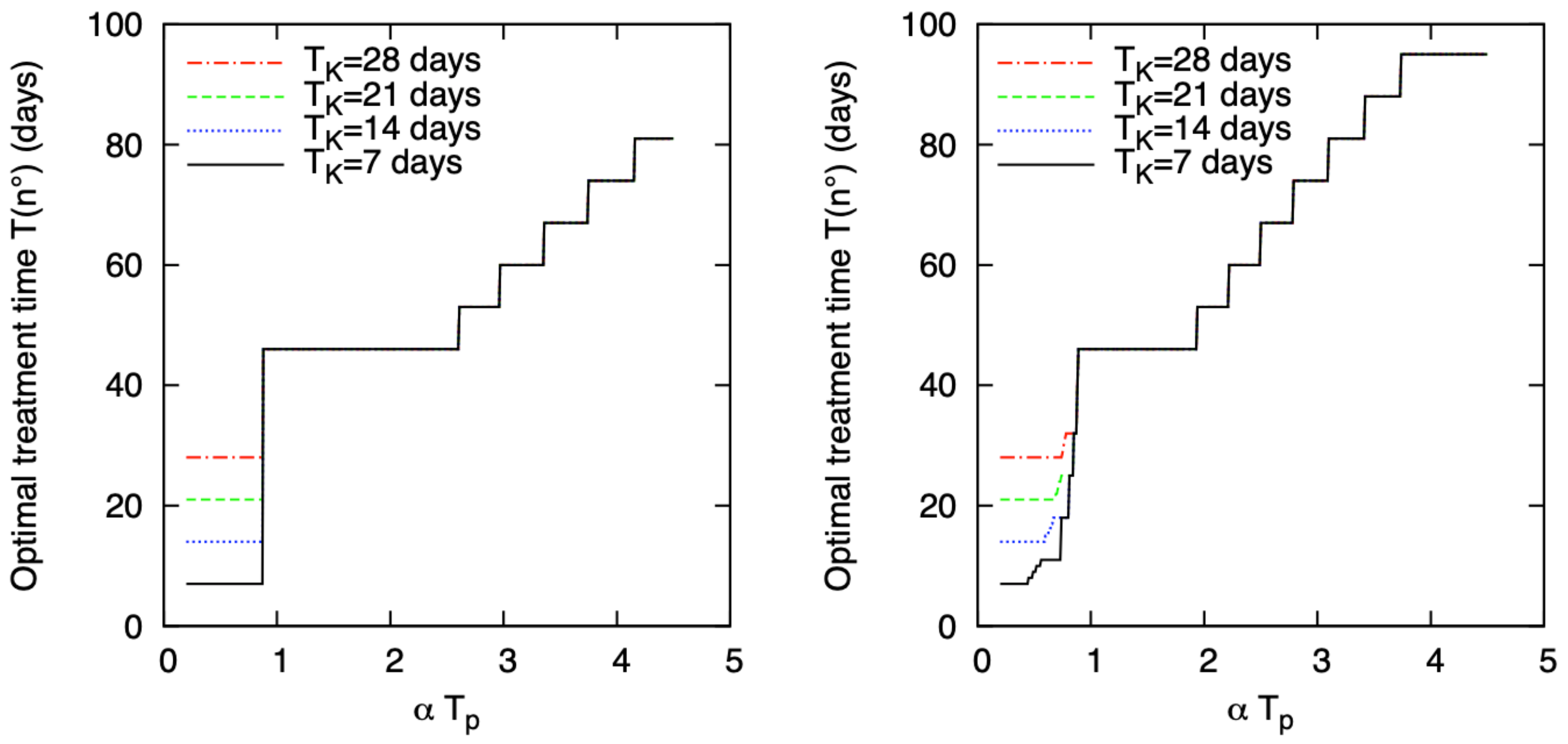
For fast proliferating tumors, the optimal fractionation scheme is uniform and made of fractions equal to $\overline{d}$. By contrast, as observed by some authors, the optimal treatment length is affected by $T_K$ and $T_P$ (actually by $\alpha T_P$) [4,5]. Figure 4 shows the optimal treatment time as a function of the product $\alpha T_P$ for $T_K=7$, 14, 21, and 28 days. Moreover, $\rho =10$ (left) and 50 Gy (right), and $d_M=7$ Gy. Taking into account that most typically the average $\alpha T_P$ ranges in [1, 2.5] Gy${}^{-1}·$ days, the most recurrent $T\left(n^{\circ }\right)$ is 46 days equal to the reference protocol duration. For very small $\alpha T_P$, schedules shorter than the standard reference are preferable and in particular as close as possible to $T_K$. When $\alpha T_P$ is large, protracting the treatment time can be advantageous.

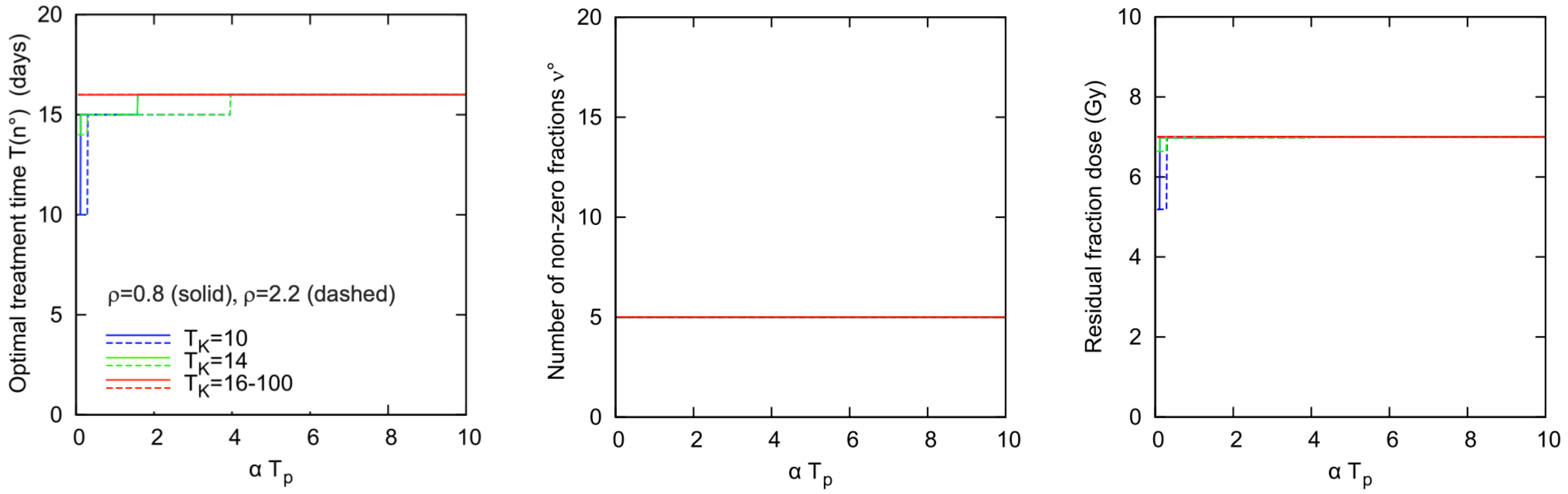
For tumors with low radiosensitivity ratios ($\rho <{\rho }_l$), the optimal solution tends to be hypofractionated, i.e., composed by few fractions of large size, and in principle it would be made by a single fraction if $d_M$ could exceed $min\{{\overline{A}}_e(1,0),A_l(1,0)\}$. Hence, the choice of the limit $d_M$ is expected to strongly affect the optimal schedule. Higher tumor cell kill and lower normal tissue $\mathrm{BED}$ can be achieved using hypofractionated regimes rather than the conventional ones, provided that $d_M$ can be safely increased.

Figure 5 shows the optimal solution for the class $\rho <{\rho }_l$ as a function of $\alpha T_P$ for $d_M=7$ Gy. For this class, the optimal protocol is completely specified by the triple $n^{\circ }$ (or $T\left(n^{\circ }\right)$), number of non-zero fractions at optimum ${\nu }^{\circ }$, size of the “residual fraction". In fact, we remind that the optima of this class take the form $d_l(1,u)$ or $d_e(1,u)$, where u depends on $d_M$ and is such that $u+1={\nu }^{\circ }\le n^{\circ }$ (see Table 8, Table 9 and Table 10) and the residual fraction is the only fraction different from zero and from $d_M$. We add some comments to Figure 5. First, the optimal treatment time of 16 days is the minimal time allowing to satisfy the early tissue constraint with the equality sign. Second, and perhaps more interesting, for most of the considered parameter values, the plots of Figure 5 give a sharp indication of the optimum scheme of fractionation. Thus, when $\rho <{\rho }_l$, our simulation indicates that the optimal solution is substantially insensitive to variations of the tumor parameters (for fixed values of the normal tissue parameters and $d_M$), which can be considered a very favorable feature of the problem under study, in view of the high heterogeneity of tumors and of the large uncertainty affecting the estimation of tumor parameters. Clearly, from a modeling point of view, the problem shifts towards that of accurately assessing the healthy tissue constraints and the related bounds on the tolerable radiation damage, as well as the value of $d_M$.

However, for the case considered here of two quadratic normal tissue constraints with fixed parameters and a given $d_M$, the numerical simulation suggests that a single radiotherapy protocol can be adopted for the class $\rho <{\rho }_l$. The mentioned protocol holds almost everywhere in tumor parameter interval, while it possibly represents a sub-optimal solution for some parameter value. We also observe that such a robust solution is a safe solution since it is in compliance with the normal tissue constraints for any considered set of tumor parameters.

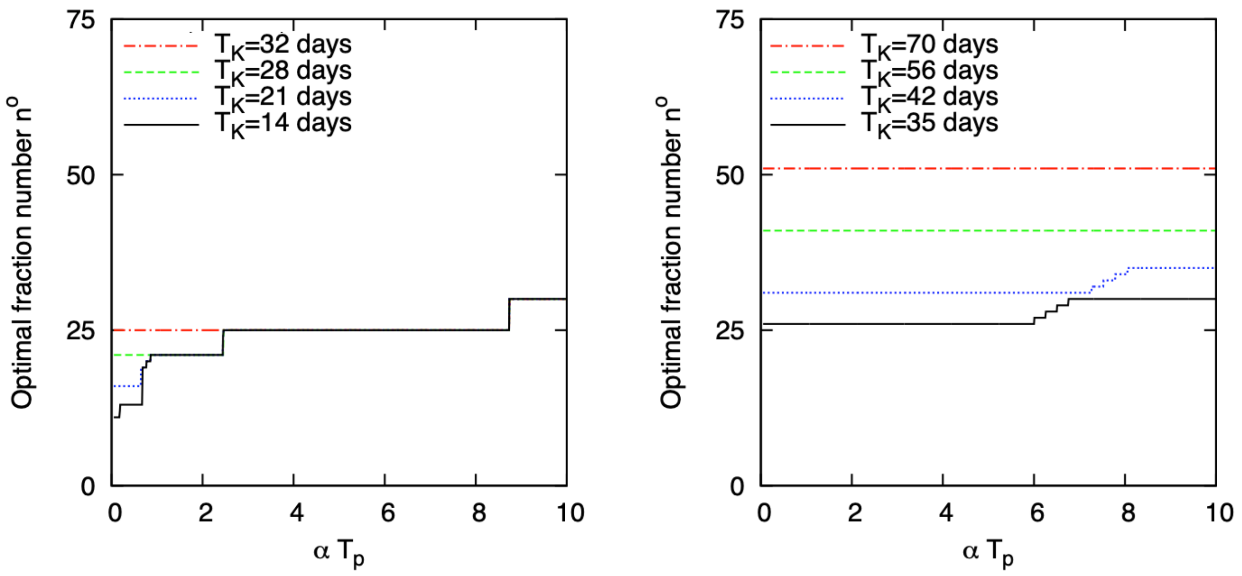
For intermediate $\rho$ values, ${\rho }_l\le \rho <{\rho }_e$, the optimal $n^{\circ }$ as a function of $\alpha T_P$, for different values of $T_K$, for $\rho =4$ Gy and setting $d_M=2.5$ Gy is reported in Figure 6. As before, all parameters have been set as the most recurrent in the literature. However, they are very scattered so that we expect to find different types of optimal schedules.

Depending on $T_K$ being shorter (left) or longer (right) than the total reference protocol time $\overline{T}$, the optimum is of the kind $d^R$, with $n^{\circ }=21$ or 25 for the majority of $\alpha T_P$ values (from 0.86 to 8.73 days/Gy). For small $\alpha T_P$, $n^{\circ }$ is smaller than the number of fractions of the reference protocol ($\overline{n}=25$) and the solution can be either $\tilde{d}$ (the vector with all $d_M$ entries) or of the kind $d_e(1,u)$, depending on $d_M$. As depicted in Figure 6 right panel, when $T_K>\overline{T}$, $T\left(n^{\circ }\right)$ turns out to be slightly greater or equal to $T_K$ for almost any $\alpha T_P$. Overall, the plots of Figure 6 show that the optimal solutions are longer than the reference ($n^{\circ }\ge \overline{n}$) and with fraction doses smaller than $\overline{d}$, which also implies that they are not affected by different $d_M$ choices. However, protracting the solution beyond $\overline{n}$ does not provide significant advantages in terms of LCK. Hence, in view of the scarceness of information about the “real” parameter values, treating tumors with intermediate proliferative behavior by means of standard fractionation schemes appears to be advantageous.

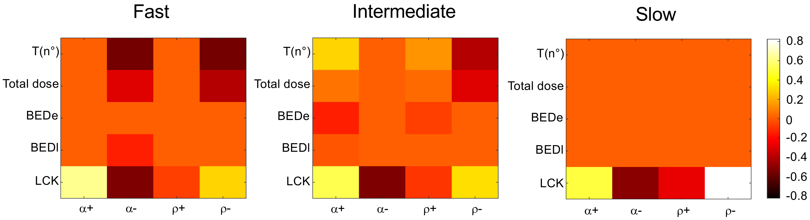
A final schematic view of the optimal protocol sensitivity for the tumor classes considered thus far is given in Figure 7.

We applied relative perturbations of ±50% to the nominal values of $\alpha$ and $\rho$, computing the relative variations of the following output quantities at the optimum: total treatment time, total dose, normal tissues damages (BED${}_l$, BED${}_e$), and tumor LCK. For all tumor classes, the resulting LCK is the quantity that exhibits the most consistent relative variations, either positive or negative, and, in particular, it can be remarkably improved (up to 80% for slow proliferating tumors upon a −50% variation of $\rho$). Apart from the LCK variation at the optimum, as also shown by Figure 4, Figure 5 and Figure 6, the solution for slow tumors is practically insensitive to the considered parameter variations, while the optimal solution for fast tumors is affected only by negative variations of $\alpha$ and $\rho$. For the class of intermediate tumors, upon both positive and negative ±50% parameter variations, we get output variations less than 30%. This is not surprising from the mathematical point of view, indicating that tumors with intermediate $\rho$ can turn into the adjacent classes of fast or of slowly proliferating tumors.

We observe that $T\left(n^{\circ }\right)$ and the optimal total dose are moderately affected by the relative parameter variations, at least for slow and, in part, for intermediate tumors. On the contrary, for fast and intermediate tumors, significant variations for $T\left(n^{\circ }\right)$ (up to −54%, see Figure 7, fast tumors panel, ${\alpha }^{-}$ and ${\rho }^{-}$ columns) accompanied by noticeable variations of the optimal total dose (up to −35%) are obtained when the optimum $T\left(n^{\circ }\right)$ tends to equal the kick-off time (21 and 28 days, respectively) unlike the conventional reference time of 35 days. Finally, reminding that the optima for all tumor types maximize at least one of the prescribed normal tissue BEDs, we verify that at least one between BED${}_l$ and BED${}_e$ is unaffected by the parameter variations, while the other shows only small (obviously negative) variations not larger than −15%.

7. Concluding Remarks

The present work illustrates an example of the application of fundamental principles of finite-dimensional nonlinear optimization to a problem of relevant interest in the clinical practice, which is the problem of finding the best fractionation scheme in cancer EBRT treatment. We present in a unitary framework an overview of the main results of our previous studies [7,8,9]. The problem formulation is based on the LQ model describing the instantaneous relation between radiation dose and cell survival for homogeneous cell populations. The model incorporates exponential repopulation, but the analytical results for n fixed are in principle valid for different modeling choices of the time-varying part of the cell population response. In its more general version, the optimization problem includes a variable number of treatment sessions and it is a mixed-integer problem that can be solved by means of two consecutive steps: (i) an analytical step to express the optimal size of the fractional doses as a function of the model parameters for a fixed, but arbitrarily chosen, number of fractions n; and (ii) a numerical step to simulate a sequence of optima obtained in Step (i) for n increasing in order to find the optimal treatment time for specific tumor types.

Concerning Step (i), we present a few versions of the problem formulation following the chronological order of the activity of our research group in this field. Our approach provides a framework to analytically determine the optimal fractionation of the total radiation dose as a function of tumor type for any arbitrarily fixed integer number of fractions. On the basis of KKT optimality conditions, we classify the optimal solutions according to the tumor radiosensitivity ratio ($\alpha /\beta$) and to the possibly imposed upper limit on the dose fraction size ($d_M$). We express the optimal fraction sizes as a function of the normal tissue parameters, recognizing the crucial role of $\alpha /\beta$ on the fractionation scheme for different tumor types. In particular, we confirm the convenience of adopting hypofractionated schedules for small $\alpha /\beta$ (i.e., slowly proliferating tumors), as previously evidenced by many authors [4,32,45], and uniform schedules of the kind commonly used in the clinical practice in any other case.

The second step implements the numerical search of the optimal number of treatment sessions, focusing on three classes of tumor types characterized by specific ranges of the radiosensitivity ratio. The numerical results confirm the influence, highlighted above, of the ratio $\alpha /\beta$ on the fractionation scheme. Recognizing that the uncertainty affecting the parameter estimation, especially in heterogeneous neoplastic cell populations, can constitute a drawback for the application of our approach, we let the tumor parameters vary in broad ranges of parameter values trying, at the same time, to provide a schematic summary of the results [9]. In particular, the numerical simulations have evidenced the role of the product $\alpha T_P$ in the optimality of treatment duration. The quantity $1/\left(\alpha T_P\right)$ can be seen as an indicator of the tumor aggressiveness, since it takes high values when rapid tumor repopulation is associated to low intrinsic radiosensitivity. Here, we present an excerpt from previous simulations reporting the optimal solution as a function of the product $\alpha T_P$. Based on the discriminating role of $\alpha T_P$, a remarkable results of our simulations is that for the majority of $\alpha T_P$ values and for the three tumor classes considered, basically two fractionated schedules appear to be preferable; for $\rho \ge {\rho }_e$, the conventional clinical protocols (e.g., the “strong standard” 2 Gy protocol) are optimal, while, for $\rho <{\rho }_l$, hypofractionated protocols are generally preferable. Moreover, if experimental or clinical evidence indicates very low $\alpha T_P$ values, shorter protocols with overall duration close to $T_K$ and/or hyperfractionation may be optimal. Indeed, in [9], we obtained optimal schemes delivering multiple fractions per day (and with treatment length near $T_K$) providing reduced late toxicity and increased tumor damage with respect to protocols with a single daily fraction. In addition, the sensitivity of the optimal solutions to $\pm 50\%$ variations of $\alpha$ and $\rho$ around their nominal values was evaluated. We stress that such a sensitivity analysis can be of some interest since the practical estimation of the radiosensitivity parameters can be critically affected by consistent estimation errors. With the only exception of the cases of $T\left(n^{\circ }\right)$ approximating $T_K$, which can occur for fast tumors with low $\alpha$ or $\rho$, the sensitivity analysis revealed that the optimal protocol variations are rather limited, with absolute variations of $T\left(n^{\circ }\right)$ and of the optimal total dose lower than 15%.

We acknowledge that our results rely on some simplifying modeling assumptions such as, in primis, the representation of the tissue response by means of the standard LQ model based on a deterministic dose–response function with four parameters. The same LQ formalism is used to model the normal tissue response and to set suitable boundary levels of the constraints necessary to ensure treatment safety. This can be considered too simplistic, especially in regard to the many biological processes involved in the normal tissue regeneration. The description of the radiation-induced damage to normal tissue and of the subsequent healing kinetics, as well as the description of the post-irradiation toxicity, are modeling issues really worthy of investigation as far as we are concerned with the optimization of cancer treatments. As an example of more sophisticated normal tissue representation, we mention the mechanistic approach by Hanin and Zaider [52] who combined a deterministic model of the normal tissue kinetics with a stochastic representation of the inter-patient variation of kinetic parameters. However, despite the criticism, the simple exponential law, starting after a “kick-off” time from the treatment beginning, has been and continues to be largely used to model the tumor repopulation, as well as to predict the tolerable radiation levels of acute reactions in healthy tissues (see, e.g., [4,5,11,35,42]).

Thus, concerning the normal tissue constraints, we assume the maximal tolerable levels for early and late complications, as well as the fraction limit $d_M$, as input data values of the optimization procedure. Furthermore, the quantities $k_e\left(n\right)$ and $k_l$ (or $h_e$ and $h_l$) have been expressed by means of the Biologically Effective Dose to evaluate the extreme boundaries of early and late side-effects. Then, these values are dependent on the model used to represent the damage and on a known tolerable clinical protocol set as the reference protocol. At present, this kind of representation based on the BED formalism is very frequently adopted and applied in planning external beam radiation treatments, at least for the management of early-stage disease cases [24].

Finally, the modeling framework based on few “essential” parameters adopted in the present study, allowed us to give a remarkably synthetic picture of the results of the optimal radiotherapy problem. These results were obtained from the application of fundamental principles of the nonlinear optimization and appear to be in good agreement with observations reported in the theoretical and clinical literature.

References

1. Tannock, I.F.; Goldenberg, G.J. Drug resistance and experimental chemotherapy. In The Basic Science of Oncology; Tannock, I.F., Hill, R.P., Eds.; McGraw-Hill: New York, NY, USA, 1998; pp. 392–419. [Google Scholar]
2. Prasanna, P.G.S.; Stone, H.B.; Wong, R.S.; Capala, J.; Bernhard, E.J.; Vikram, B.; Coleman, C.N. Normal tissue protection for improving radiotherapy: Where are the Gaps? Transl. Cancer Res. 2012, 1, 35–48. [Google Scholar] [PubMed]
3. Fowler, J.F. 21 years of Biologically Effective Dose. Br. J. Radiol. 2010, 83, 554–568. [Google Scholar] [CrossRef] [PubMed]
4. Fowler, J.F. Practical time-dose evaluations, or how to stop worrying and learn to love linear quadratics. In Technical Basis of Radiation Therapy; Levitt, S.H., Purdy, J.A., Perez, C.A., Poortmans, P., Eds.; Springer-Verlag: Berlin, Germany, 2012; pp. 3–50. [Google Scholar]
5. Yang, Y.; Xing, L. Optimization of radiotherapy dose-time fractionation with consideration of tumor specific biology. Med. Phys. 2005, 32, 3666–3677. [Google Scholar] [CrossRef] [PubMed]
6. Jones, B.; Dale, R.G. Mathematical models of tumour and normal tissue response. Acta Oncol. 1999, 38, 883–893. [Google Scholar] [CrossRef] [PubMed]
7. Bertuzzi, A.; Bruni, C.; Papa, F.; Sinisgalli, C. Optimal solution for a cancer radiotherapy problem. J. Math. Biol. 2013, 66, 311–349. [Google Scholar] [CrossRef] [PubMed]
8. Bruni, C.; Conte, F.; Papa, F.; Sinisgalli, C. Optimal weekly scheduling in fractionated radiotherapy: Effect of an upper bound on the dose fraction size. J. Math. Biol. 2015, 71, 361–398. [Google Scholar] [CrossRef] [PubMed]
9. Bruni, C.; Conte, F.; Papa, F.; Sinisgalli, C. Optimal dose size and number in fractionated radiotherapy. Math. Med. Biol. 2019, 36, 1–53. [Google Scholar] [CrossRef] [PubMed]
10. Lee, E.K.; Fox, T.; Crocker, I. Simultaneous beam geometry and intensity map optimization in intensity-modulated radiation therapy. Int. J. Radiat. Oncol. Biol. Phys. 2006, 64, 301–320. [Google Scholar] [CrossRef] [PubMed]
11. Saberian, F.; Ghate, A.; Kim, M. Optimal fractionation in radiotherapy with multiple normal tissues. Math. Med. Biol. 2015, 32, 211–252. [Google Scholar]
12. Fowler, J.F. The linear-quadratic formula and progress in fractionated radiotherapy. Br. J. Radiol. 1989, 62, 679–694. [Google Scholar] [CrossRef] [PubMed]
13. Thames, H.D. An ‘incomplete-repair’ model for survival after fractionated and continuous irradiations. Int. J. Radiat. Biol. 1985, 47, 319–339. [Google Scholar] [CrossRef] [PubMed]
14. Hlatky, L.R.; Hahnfeldt, P.; Sachs, R.K. Influence of time-dependent stochastic heterogeneity on the radiation response of a cell population. Math. Biosci. 1994, 122, 201–220. [Google Scholar] [CrossRef]
15. Brenner, D.J.; Hlatky, L.R.; Hahnfeldt, P.J.; Hall, E.J.; Sachs, R.K. A convenient extension of the linear-quadratic model to include redistribution and reoxygenation. Int. J. Radiat. Oncol. Biol. Phys. 1995, 32, 379–390. [Google Scholar] [CrossRef]
16. Brenner, D.J. The linear-quadratric model is an appropriate methodology for determining isoeffective doses at large doses per fraction. Semin. Radiat. Oncol. 2008, 18, 234–239. [Google Scholar] [CrossRef] [PubMed] [Green Version]
17. Kirkpatrick, J.P.; Meyer, J.J.; Marks, L.B. The linear-quadratric model is inappropriate to model high dose per fraction effects in radiosurgery. Semin. Radiat. Oncol. 2008, 18, 240–243. [Google Scholar] [CrossRef] [PubMed]
18. Kirkpatrick, J.P.; Brenner, D.J.; Orton, C.G. Point/counterpoint. The linear-quadratric model is inappropriate to model high dose per fraction effects in radiosurgery. Med. Phys. 2009, 36, 3381–3384. [Google Scholar] [CrossRef] [PubMed] [Green Version]
19. Astrahan, M. Some implications of linear-quadratic-linear radiation dose-response with regard to hypofractionation. Med. Phys. 2008, 35, 4161–4172. [Google Scholar] [CrossRef] [PubMed] [Green Version]
20. Guerrero, M.; Li, X.A. Extending the linear-quadratic model for large fraction doses pertinent to stereotactic radiotherapy. Phys. Med. Biol. 2004, 49, 4825–4835. [Google Scholar] [CrossRef] [PubMed]
21. Hanin, L.G.; Zaider, M. Cell-survival probability at large doses: An alternative to the linear-quadratic model. Phys. Med. Biol. 2010, 55, 4687–4702. [Google Scholar] [CrossRef] [PubMed]
22. Alfonso, J.C.L.; Berk, L. Modeling the effect of intratumoral heterogeneity of radiosensitivity on tumor response over the course of fractionated radiation therapy. Radiat. Oncol. 2019, 14, 88. [Google Scholar] [CrossRef] [PubMed] [Green Version]
23. Brown, J.M. The biology of SBRT: LQ or something new? Int. J. Radiat. Oncol. Biol. Phys. 2018, 101, 964. [Google Scholar] [CrossRef] [PubMed]
24. Dearnaley, D.; Syndikus, I.; Mossop, H.; Khoo, V.; Birtle, A.; Bloomfield, D.; Graham, J.; Kirkbride, P.; Logue, J.; Malik, Z.; et al. Conventional versus hypofractionated high-dose intensity-modulated radiotherapy for prostate cancer: 5-year outcomes of the randomised, non-inferiority, phase 3 CHHiP trial. Lancet Oncol. 2016, 17, 1047–1060. [Google Scholar] [CrossRef] [Green Version]
25. Lewin, T.D.; Maini, P.K.; Moros, E.G.; Enderling, H.; Byrne, H.M.; Zaider, M.; Hanin, L.G. The evolution of tumour composition during fractionated radiotherapy: Implications for outcome. Bull. Math. Biol. 2018, 80, 1207–1235. [Google Scholar] [CrossRef] [PubMed] [Green Version]
26. Van Leeuwen, C.M.; Oei, A.L.; Crezee, J.; Bel, A.; Franken, N.A.P.; Stalpers, L.J.A.; Kok, H.P. The alfa and beta of tumours: A review of parameters of the linear-quadratic model, derived from clinical radiotherapy studies. Radiat. Oncol. 2018, 13, 1–11. [Google Scholar] [CrossRef] [PubMed]
27. Fowler, J.F. Optimum overall times II: Extended modelling for head and neck radiotherapy. Clin. Oncol. 2008, 20, 113–126. [Google Scholar] [CrossRef] [PubMed]
28. O’Rourke, S.F.C.; McAneney, H.; Hillen, T. Linear quadratic and tumour control probability modelling in external beam radiotherapy. J. Math. Biol. 2009, 58, 799–817. [Google Scholar] [CrossRef] [PubMed]
29. Halperin, E.C.; Wazer, D.E.; Perez, C.A.; Brady, L.W. Perez and Brady’s Principles and Practice of Radiation Oncology; Lippincott Williams Wilkins: Philadelphia, PA, USA, 2013. [Google Scholar]
30. Oliveira, M.; Teixeira, N.J.; Fernandes, L. What do we know about the α/β for prostate cancer? Med. Phys. 2012, 39, 3189–3201. [Google Scholar] [CrossRef] [PubMed]
31. Pierre, D.A. Optimization Theory with Applications; John Wiley & Sons: New York, NY, USA, 1969. [Google Scholar]
32. Brenner, D.J.; Hall, E.J. Fractionation and protraction for radiotherapy of prostate carcinoma. Int. J. Radiat. Oncol. Biol. Phys. 1999, 43, 1095–1101. [Google Scholar] [CrossRef]
33. Fowler, J.F.; Ritter, M.A.; Chappel, R.J.; Brenner, D.J. What hypofractionated protocols should be tested for prostate cancer? Int. J. Radiat. Oncol. Biol. Phys. 2003, 56, 1093–1104. [Google Scholar] [CrossRef]
34. Badri, H.; Pitter, K.; Holland, E.C.; Michor, F.; Leder, K. Optimization of radiation dosing schedules for proneural glioblastoma. J. Math. Biol. 2016, 72, 1301–1336. [Google Scholar] [CrossRef] [PubMed]
35. Badri, H.; Watanabe, Y.; Leder, K. Optimal radiotherapy dose schedules under parametric uncertainty. Phys. Med. Biol. 2016, 61, 338–364. [Google Scholar] [CrossRef] [PubMed]
36. Mizuta, M.; Takao, S.; Date, H.; Kishimoto, N.; Sutherland, K.L.; Onimaru, R.; Shirato, H. A mathematical study to select fractionation regimen based on physical dose distribution and the linear-quadratic model. Int. J. Radiat. Oncol. Biol. Phys. 2012, 84, 829–833. [Google Scholar] [CrossRef] [PubMed] [Green Version]
37. Saberian, F.; Ghate, A.; Kim, M. A two-variable linear program solves the standard linear-quadratic formulation of the fractionation problem in cancer radiotherapy. Oper. Res. Lett. 2015, 43, 254–258. [Google Scholar] [CrossRef]
38. Unkelbach, J.; Craft, D.; Salari, E.; Ramakrishnan, E.; Bortfeld, T. The dependence of optimal fractionation schemes on the spatial dose distribution. Phys. Med. Biol. 2013, 58, 159–167. [Google Scholar] [CrossRef] [PubMed] [Green Version]
39. Barendsen, G.W. Dose fractionation, dose rate, and isoeffect relationships for normal tissue responses. Int. J. Radiat. Oncol. Biol. Phys. 1982, 8, 1981–1997. [Google Scholar] [CrossRef]
40. Ling, C.C.; Gerweck, L.E.; Zaider, M.; Yorke, E. Dose-rate effects in external beam radiotherapy redux. Radiother. Oncol. 2010, 95, 261–268. [Google Scholar] [CrossRef] [PubMed]
41. Macchia, G.; Ferrandina, G.; Deodato, F.; Ruggieri, V.; Massaccesi, M.; Salutari, V.; Valentini, V.; Cellini, N.; Scambia, G.; Morganti, A.G. Concomitant boost dose escalation plus large-field preoperative chemoradiation in locally advanced carcinoma of the uterine cervix: Results of a phase i study (LARA-CC-1). Gynecol. Oncol. 2010, 118, 128–133. [Google Scholar] [CrossRef]
42. Fowler, J.F.; Harari, P.M.; Leborgne, F.; Leborgne, J.H. Acute radiation reactions in oral and pharyngeal mucosa: Tolerable levels in altered fractionation schedules. Radiother. Oncol. 2003, 69, 161–168. [Google Scholar] [CrossRef]
43. Thames, H.D.; Bentzen, S.M.; Turesson, I.; Overgaard, M.; van den Bogaert, W. Time-dose factors in radiotherapy: A review of the human data. Radiother. Oncol. 1990, 19, 219–235. [Google Scholar] [CrossRef]
44. Dasu, A.; Toma-Dasu, I. Prostate alpha/beta revisited—An analysis of clinical results from 14,168 patients. Acta Oncol. 2012, 51, 963–974. [Google Scholar] [CrossRef]
45. Fowler, J.F. Biological factors influencing optimum fractionation in radiation therapy. Acta Oncol. 2001, 40, 712–717. [Google Scholar] [CrossRef] [PubMed]
46. Fowler, J.F.; Toma-Dasu, I.; Dasu, A. Is the α/β ratio for prostate tumours really low and does it vary with the level of risk at diagnosis? Anticancer Res. 2013, 33, 1009–1012. [Google Scholar] [PubMed]
47. Gao, M.; Mayr, N.A.; Huang, Z.; Zhang, H.; Wang, J.Z. When tumor repopulation starts? The onset time of prostate cancer during radiation therapy. Acta Oncol. 2010, 49, 1269–1275. [Google Scholar] [CrossRef] [PubMed]
48. Miralbell, R.; Roberts, S.A.; Zubizarreta, E.; Hendry, J.H. Dose-fractionation sensitivity of prostate cancer deduced from radiotherapy outcomes of 5969 patients in seven international institutional datasets: α/β = 1.4 (0.9–2.2) Gy. Int. J. Radiat. Oncol. Biol. Phys. 2012, 82, e17–e24. [Google Scholar] [CrossRef] [PubMed]
49. Proust-Lima, C.; Taylor, J.M.; Secher, S.; Sandler, H.; Kestin, L.; Pickles, T.; Bae, K.; Allison, R.; Williams, S. Confirmation of a low α/β ratio for prostate cancer treated by external beam radiation therapy alone using a post-treatment repeated-measures model for PSA dynamics. Int. J. Radiat. Oncol. Biol. Phys. 2011, 79, 195–201. [Google Scholar] [CrossRef] [PubMed] [Green Version]
50. Nahum, A.E.; Movsas, B.; Horwitz, E.M.; Stobbe, C.C.; Chapman, J.D. Incorporating clinical measurements of hypoxia into tumor local control modeling of prostate cancer: Implications for the α/β ratio. Int. J. Radiat. Oncol. Biol. Phys. 2003, 57, 391–401. [Google Scholar] [CrossRef]
51. Wang, J.Z.; Li, X.A. Impact of tumor repopulation on radiotherapy planning. Int. J. Radiat. Oncol. Biol. Phys. 2005, 61, 220–227. [Google Scholar] [CrossRef] [PubMed]
52. Hanin, L.G.; Zaider, M. A mechanistic description of radiation-induced damage to normal tissue and its healing kinetics. Phys. Med. Biol. 2013, 58, 825–839. [Google Scholar] [CrossRef] [PubMed]
Figure 1. Qualitative geometrical representation illustrating Theorem 2 for n = 2 and n = 3 .
Information 11 00313 g001
Figure 2. Optimal fractions d i , i = 1 , , 5 , for prevalent late constraint and ρ < ρ l (see Table 7): (Top) patterns of the dose fractions as functions of d M ; and (Bottom) optimal weekly schedules (vertical bars) corresponding to significant values of d M (limiting horizontal lines).
Information 11 00313 g002
Figure 3. Qualitative example for n = 3 to illustrate the optima of Table 8. Behavior of the optimal solution for a tumor with ρ < ρ l in the absence of a prevalent constraint and for two d M values: (Left) d M > A l ( 1 , 0 ) ; and (Right) A l ( 2 , 0 ) < d M < A l ( 1 , 0 ) .
Information 11 00313 g003
Figure 4. Optimal treatment time T ( n ) as a function of α T P for ρ = 10 Gy (left) and for ρ = 50 Gy (right). Daily dose upper bound d M = 7 Gy.
Information 11 00313 g004
Figure 5. Optimal protocols for slowly proliferating tumors, ρ < ρ l , as a function of α T P , for different ρ and T K . Daily dose upper bound d M = 7 Gy.
Information 11 00313 g005
Figure 6. Optimal protocols for tumors with intermediate ρ ( ρ = 4 Gy) as a function of α T P , for different T K . Reference protocol: 25 F × 1.8 Gy = 45 Gy / 32 days: (Left) T K T ¯ ; and (Right) T K > T ¯ , with T ¯ total reference protocol time. Daily dose upper bound d M = 2.5 Gy.
Information 11 00313 g006
Figure 7. Sensitivity of optimal fractionated protocols to ±50% variations of α and ρ around the nominal values, for the considered tumor classes. Nominal parameter values: ρ = 10 Gy, α = 0.35 Gy 1 , T K = 21 days, and T P = 3 days (Fast); ρ = 6 Gy, α = 0.2 Gy 1 , T K = 28 days, and T P = 14 days (Intermediate); and ρ = 1.5 Gy, α = 0.1 Gy 1 , T K = 35 days, and T P = 28 days (Slow). d M = 7 Gy.
Information 11 00313 g007