Evaluation of Tree-Based Ensemble Machine Learning Models in Predicting Stock Price Direction of Movement


School of Information and Software Engineering, University of Electronic Science and Technology of China (UESTC), Chengdu 610051, China
*
Author to whom correspondence should be addressed.
Information 2020, 11(6), 332; https://0-doi-org.brum.beds.ac.uk/10.3390/info11060332
Submission received: 24 May 2020
/
Revised: 14 June 2020
/
Accepted: 17 June 2020
/
Published: 20 June 2020
(This article belongs to the Special Issue Machine Learning on Scientific Data and Information)
Abstract
:Forecasting the direction and trend of stock price is an important task which helps investors to make prudent financial decisions in the stock market. Investment in the stock market has a big risk associated with it. Minimizing prediction error reduces the investment risk. Machine learning (ML) models typically perform better than statistical and econometric models. Also, ensemble ML models have been shown in the literature to be able to produce superior performance than single ML models. In this work, we compare the effectiveness of tree-based ensemble ML models (Random Forest (RF), XGBoost Classifier (XG), Bagging Classifier (BC), AdaBoost Classifier (Ada), Extra Trees Classifier (ET), and Voting Classifier (VC)) in forecasting the direction of stock price movement. Eight different stock data from three stock exchanges (NYSE, NASDAQ, and NSE) are randomly collected and used for the study. Each data set is split into training and test set. Ten-fold cross validation accuracy is used to evaluate the ML models on the training set. In addition, the ML models are evaluated on the test set using accuracy, precision, recall, F1-score, specificity, and area under receiver operating characteristics curve (AUC-ROC). Kendall W test of concordance is used to rank the performance of the tree-based ML algorithms. For the training set, the AdaBoost model performed better than the rest of the models. For the test set, accuracy, precision, F1-score, and AUC metrics generated results significant to rank the models, and the Extra Trees classifier outperformed the other models in all the rankings.
1. Introduction
Forecasting future the trend and direction of stock price movement is an essential task which helps investors to take prudent financial decisions in the stock (equity) market. However, carrying out such task is very exacting since factors (such as political events, economic factors, investors’ sentiments, etc.) that influence the behavior of the equity market change constantly at a great pace, and they are greatly affected by the high degree of noise [1]. For many years, investors and researchers were of the belief that the stock price cannot be predicted. This belief came into existence due to random walk theory [2,3,4] and the efficient market hypothesis (EMH) [5,6]. Supporters of the random walk theory have the belief that stock prices will move along a random walk path and any forecast of the movement of stock will be about fifty percent (50%) [7]. Also, EMH posits that, the equity market reflects every currently available information, hence, it cannot be forecasted to consistently make economic gains that surpass the overall market average. However, numerous research studies have provided evidence to the contrary, to show that the equity market can be forecasted to some extent [8,9,10,11]. Investors have been able to gain profit by beating the market [12]. Investing in equity markets has big risk associated with it due to the fact that financial market time series are non-parametric, dynamic, noisy, and chaotic. To be able to minimize the associated risk of equity market investment, a foreknowledge on the future movement of stock price is needed. A precise forecast of equity market movement is essential in order to maximize capital gain and minimize loss, since investors are likely to buy or desist from stock whose future value is expected to rise or fall respectively. Methods such as technical analysis, fundamental analysis, time series forecasting, and machine learning (ML) exist to forecast the behavior of stock prices. In this paper, we focus on the use of ML to predict stock price behavior as it is known from the literature that ML models typically produce better results than statistical and econometric models [13,14,15], and it captures the non-linear nature of the equity market better than the other methods. Also, with the availability of huge amounts of stock trading data as a result of advances in computing, the task of predicting the behavior of the equity market is too massive to be carried out with the other methods. Moreover, with ML technique, individual models can be combined to obtain a reduction in variance and improve the performance of the models [16]. Predicting stock price with ML models has two approaches: (a) using the single ML model [9,17,18,19,20,21], and (b) using ensemble ML models [16,22,23,24,25,26,27]. Application of ensemble ML models has been reported in the literature by some researchers to produce superior performance than single ML models [24,28,29]. Hence, in this article, we study tree-based ensemble ML models in an effort to predict the direction of stock price movement. Thus, our goal is to build an intelligent tree-based ensemble machine learning models that learn from the past stock market data and estimate the direction of stock price movement. Precisely, we examine and compare the effectiveness of the following tree-based ensemble ML models in forecasting the direction of stock price movement: (i) Random Forest Classifier (RF), (ii) XGBoost Classifier (XG), (iii) Bagging Classifier (BC), (iv) AdaBoost Classifier (Ada), (v) Extra Trees classifier (ET), and (vi) Voting Classifier (VC).
2. Experimental Design
In this experiment, stock data were acquired through the yahoo finance application programming interface (API). Technical indicators that reflect variations in price over time are computed. The data are subjected to two preprocessing steps: (i) data cleaning; to take care of missing and erroneous values; (ii) data normalization; to enable the machine learning models to perform well. Feature extraction technique is used to extract the relevant features for the machine learning models. The tree-based ensemble machine learning models are trained and predictions made with them. The models are evaluated and ranked using different evaluation metrics.
2.1. Data and Features
Eight stock data sets are randomly collected from three different stock exchanges (New York Stock Exchange (NYSE), National Association of Securities Dealers Automated Quotations System (NASDAQ), and National Stock Exchange of India Ltd (NSE)). The data for the following stocks are used: Bank of America Corporation (BAC), Exxon Mobil Corporation (XOM), S&P 500 Index (INX), Microsoft Corporation (MSFT), Dow Jones Industrial Average (DJIA INDEX), CarMax, Inc. (KMX), Tata Steel Limited (TATASTEEL), and HCL Technologies Ltd (HCLTECH). Table 1 presents a description of the dataset. Forty (40) technical indicators from four different categories of technical indicators (namely, momentum indicators, volume indicators, price transform, and overlap studies) are computed from the OHLCV data collected and used as input features. Details of the overlap studies, volume indicators, price transform, and momentum indicators are provided by Table A1, Table A2, Table A3 and Table A4 respectively at the Appendix A. Each dataset is divided into training and test sets for the purpose of this experiment. The training set constitute the initial 70% of the data set, and the test set is made up of the final 30% of the data set. Ten-fold cross-validation is used for the Training set. In the cross-validation, the data set is split into 10 groups. To train the model, nine out of the 10 groups are used to train the model and the remaining group is used to evaluate the performance of the model. This process is repeated 10 times with a different 10th of the dataset used to test the remaining 9 groups during every run of the 10-fold cross validation.
2.2. Data Normalization
The different features do not have the same range of values. Therefore, we normalized the input dataset to bring the values of all features in the same range. Standardization scaling (z-score) is applied to normalize the feature set. The z-score transform features so that they have characteristics of a Gaussian distribution with the values of each feature having a mean of zero and a unit-variance [30].
where = mean of the feature, = standard deviation of the feature.
2.3. Feature Extraction
The final dataset comprises of 45 predictors (40 technical indicators and the OHLCV variables). High dimensional data suffers from the curse of dimensionality which causes the performance and accuracy of learning algorithms to reduce. Hence, dimensionality reduction process is essential in the study. However, getting most of the information offered by the original features is of extreme importance. PCA is applied in this study. PCA has been shown to improve the stability and performance of models in stock prediction [31,32]. PCA operates with the aim of extracting and keeping only the most relevant information of the original dataset. It achieves this aim by employing orthogonal transformation to transform values of possibly correlated features into values of features that are linearly uncorrelated. These new features are known as principal components (PC). The PCs are linear combinations of features of the original dataset hence, the reconstruction error is greatly reduced. PCA generates orthogonal components, implying that they are not correlated to each other. The selection of the first PC is done in a way that reduces the distance between the data and its projection onto the PC. By reducing the distance, we increase the variance of the projected points. The subsequent PCs are chosen in a similar manner but with the added obligation that they should be uncorrelated with the preceding PCs. In several instances, most variance within the dataset are accounted for by the initial few PCs, therefore, the remainder of the PCs can be disregarded with only a minor information loss. Our stock market dataset appears to have many highly correlated features, hence, applying PCA helps us lessen the effect of strong correlations among features, while decreasing the dimensionality of the feature space. We used PCs that preserve most of the variance (information) of the original data, hence setting the threshold to 95%.
2.4. Machine Learning Algorithms
The effectiveness of tree-based ML ensemble models (Random Forest classifier, XGBoost classifier, AdaBoost classifier, Bagging classifier, Extra Trees classifier, and Voting classifier) in forecasting the direction of stock price movement is examined in the study. A brief discussion of these ensemble tree-based classifiers is provided here.
2.4.1. Base Classifier
In this study all the ensemble classifiers use decision tree classifier as the base classifier. A decision tree (DT) makes predictions on a target variable based on a sequence of rules set in a tree-like structure. It comprises of non-leaf node(s) representing test on an attribute, branches representing possible outcomes of the test, and leaf nodes representing class labels. Decision tree classifies a new observation by navigating them down the tree from the root to a leaf node, based on the output of the tests along the path [33]. DT follows a similar approach that human beings generally follow in making decisions. Hence, DT models are intuitive and can be explained easily.
2.4.2. Random Forest Classifier
Random Forest (RF) operates by constructing a group of decision trees to enhance the robustness and performance of the decision trees [34]. This method merges the random selection of features technique [35,36,37] and Breiman’s bagging sampling method [38], to build a group of decision trees with controlled variation. Employing bagging, each decision tree within the group is created by means of a sample with replacement from the training data. Each decision tree within the group acts as a base estimator to establish the class label of an unlabeled instance. This is accomplished through majority votes. Each of the base decision tree model casts a vote for the class label it predicted. The class label that gets majority of the votes is used to classify the instance. RF is robust to noise and overfitting [39]. The Random forest algorithm has been applied in several fields by different researchers. Some of the recent applications of random forest algorithm include random forest for label ranking [40], stock selection with random forest [41], structured random forest for label distribution learning [42], clinical risk prediction with random forests for survival, longitudinal, and multivariate (RF-SLAM) data analysis [43], and the application of random forest-based approaches to surface-enhanced Raman scattering data [44].
2.4.3. AdaBoost Classifier
AdaBoost is a boosting machine learning technique that works by combining multiple weak learners into a special classifier via a weighted linear combination. AdaBoost sequentially applies a learning algorithm to reweighted samples of the original training data [45]. It is an iterative algorithm and, in each iteration, the misclassified instances in a prior iteration are given more weight. Initially, each instance is assigned equal weight and iteration by iteration, the weights of all wrongly classified instances are raised and that of rightly classified instances are reduced. The algorithm iterates repeatedly applying the base classifier on the training data with new weights. The final classification model produced is a linear combination of all the models gotten in the different iterations [46]. AdaBoost fully considers the weight of every classifier, however, it is sensitive to outliers and noisy data. The application of AdaBoost algorithm in the literature is very diverse. Recent usages of AdaBoost include time series classification based on Arima and AdaBoost [47], an AdaBoost algorithmic method for computational financial analysis [48], and an AdaBoost classifier using stochastic diffusion search model for data optimization in Internet of Things [49].
2.4.4. XGBoost Classifier
XGBoost is a scalable and efficient variant of the gradient tree boosting algorithm. In the gradient boosting algorithm, boosting is viewed as an optimization problem with the aim of minimizing the loss function of the classification model by addition of one weaker learner at a time. The algorithm continuously minimizes errors of the previous models in the direction of gradient to produce a new model [50]. XGBoost algorithm incorporates the following features [51]: (a) regularized model to prevent overfitting (b) sparsity-aware split finding algorithm to deal with different kinds of sparsity patterns in the data (c) distributed weighted quantile sketch algorithm to deal effectively with weighted data (d) column block structure for parallel learning (e) cache-aware prefetching algorithm to fetch and store the gradient statistics (f) blocks for out-of-core computation. Recent applications of XGBoost in the literature include hard rock pillar stability forecast using GBDT, XGBoost, and LightGBM algorithms [52], gene expression value forecast based on XGBoost Algorithm [53], and the enhancement of diagnosis of depression using XGBOOST model and a large biomarkers Dutch dataset [54].
2.4.5. Bagging Classifier
A Bagging classifier is an ensemble meta-estimator. This algorithm creates multiple models by fitting each base classifier on a random subsample of the original dataset and then combine the results of all the models to determine the final prediction. The bagging classifier uses either the greatest mean probability among the base classifiers or majority voting to establish the predicted label. Since the original training dataset is re-sampled with replacement, certain instances may be selected many times while others are not selected at all. The meta-estimator reduces the variance of the base estimator through the introduction of randomization into the construction method and then generating an ensemble from it [55]. The base classifiers are trained in parallel with the subgroup of the training set generated via random selection with replacement from the original dataset. The training dataset of every base classifier is independent of the others. The Bagging algorithm has also seen extensive application in the literature. Some of the recent applications of the bagging algorithm include comparative application of Bagging and Boosting ensemble machine learning approaches for automated EMG signal classification [56], an enhancement of the performance of Bagging for classification of imbalanced datasets with evolutionary multi-objective optimization by [57].
2.4.6. Extra Trees Classifier
The Extra-Trees classifier creates a group of unpruned decision trees in accordance with the traditional top-down method. It essentially involves randomizing both attribute and cut-point selection strongly while splitting a node of a tree. In the extreme situation, it creates fully randomized trees having structures independent of the output values of the training sample. It mainly differs from other tree-based ensemble methods on two counts, which are that it splits nodes by picking cut-points fully at random, and it also uses the whole training sample (instead of bootstrap replica) to grow the trees. The predictions of all the trees are combined to establish the final prediction, through majority vote. The idea behind extra-trees classifier is that the full randomization of the cut-point and attribute together with ensemble averaging will decrease variance better than weaker randomization strategy used by other methods. The usage of all of the original training samples instead of bootstrap replicas is to decrease bias. Computational efficiency is a major strength of this algorithm [58]. Like the other algorithms, Extra trees algorithm has also seen an extensive and diverse application in the literature. Some of the recent applications include classification of land cover using Extremely Randomized Trees [59], and a multi-layer intrusion detection system with Extra Trees feature selection, extreme learning machine ensemble, and softmax aggregation [60].
2.4.7. Voting Classifier
Voting classifier combines different types of machine learning classifiers, aggregating the output of each classifier passed to it, and makes the final prediction of the class label of a new instance based on voting. The voting may be either hard or soft. In the case of hard voting simple majority voting is used. In this case, the class that gets the greatest number of votes will be selected (predicted). For soft voting, a prediction is made by averaging the class-probabilities of each classifier. The class that gets the best average probability is predicted. In this work, we adopted soft voting. Also, the tree-based ensemble classifiers are used as the base estimators for the VC.
2.5. Evaluation Metric
To evaluate performance of the ensemble ML models the following evaluation criteria are used:
(a) accuracy, (b) precision, (c) recall, (d) F1-score (e) specificity (f) area under receiver operating characteristics curve (AUC-ROC). These metrics are classical quality criteria used to quantify performance of ML models. Below are their definitions:
Accuracy: the percentage of entire instances rightly predicted by the classifier
Precision: the proportion of positive instances rightly predicted by the classifier out of all the instances predicted by the classifier as positive.
Recall: the proportion of positive instances rightly predicted by the classifier out of all the instances that are actually positive.
f1 score: presents a harmonic mean of precision and recall
Specificity: the proportion of negative instances rightly predicted by the classifier out of the total instances that are actually negative.
where tp = true positive, fp = false positive, tn = true negative, and fn = false negative,
AUC-ROC: ROC is a probability curve that displays in a graphical way the trade-off between recall and specificity. AUC measures the ability of the classifier to distinguish between the positive and negative classes. A perfect classifier will have AUC of one, and worst performing classifier will have AUC of 0.5.
3. Results and Analysis
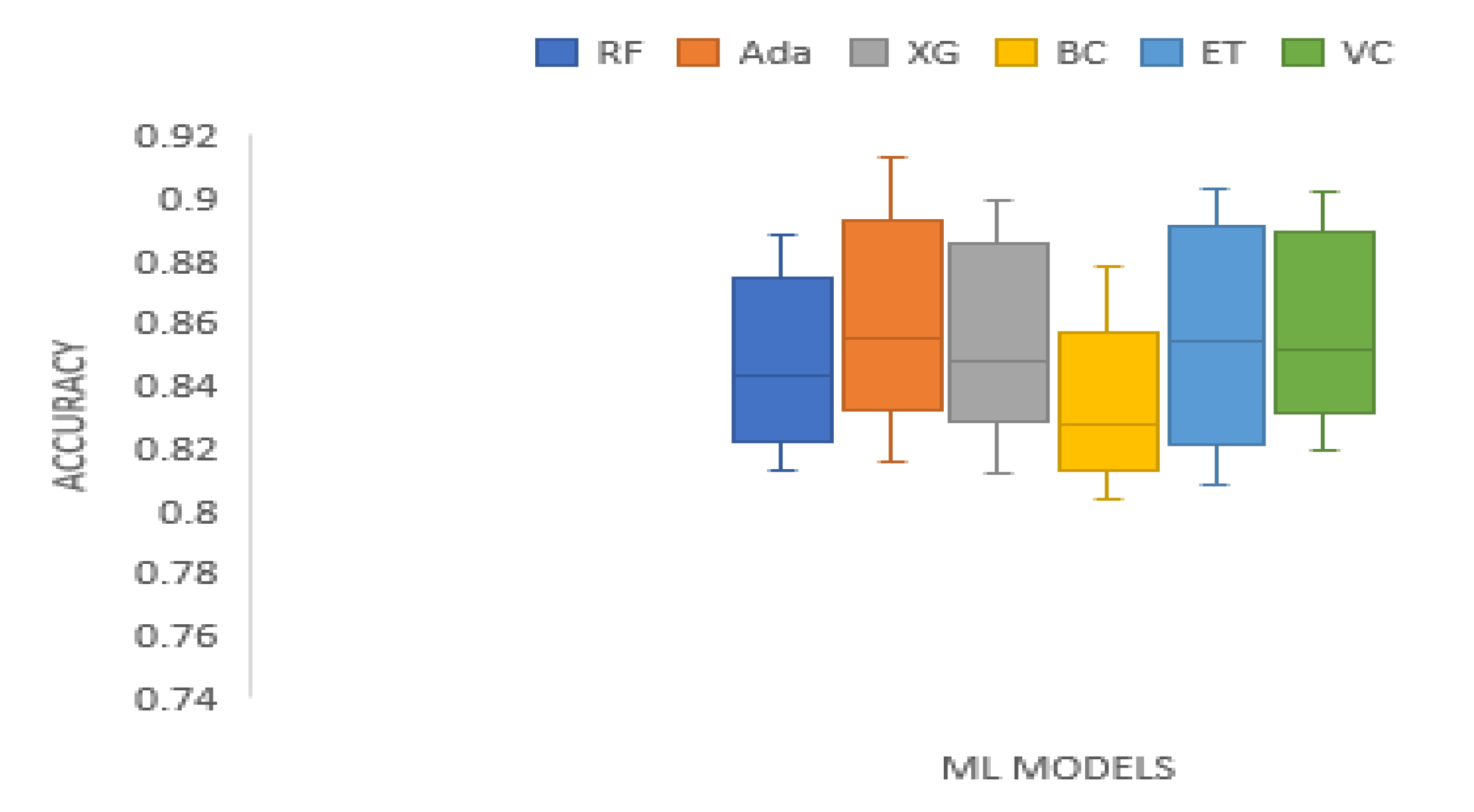
Table 2 presents the ten-fold cross validation accuracy scores of the tree-based ensemble ML models on the training set. The scores of Random Forest range from 0.8131 to 0.8884. AdaBoost scores range from 0.8157 to 0.9127. XGBoost scores range from 0.8122 to 0.8991. The accuracy scores range of Bagging classifier is from 0.8034 to 0.8781. Extra trees classifier has an accuracy score range of 0.8087 to 0.9027. The Voting classifier scores range from 0.8191 to 0.9019. The accuracy score of AdaBoost is the best on BAC, S&P_500, DJIA, KMX, TATASTEEL, and HCLTECH training datasets. Extra trees, and Voting classifiers recorded the highest accuracy on MSFT, and XOM training data sets respectively. In general, the mean accuracy of the AdaBoost model is the best among the tree-based ensemble models. A boxplot of the ten-fold cross validation accuracy scores of the ML models on the training data sets is presented by Figure 1.
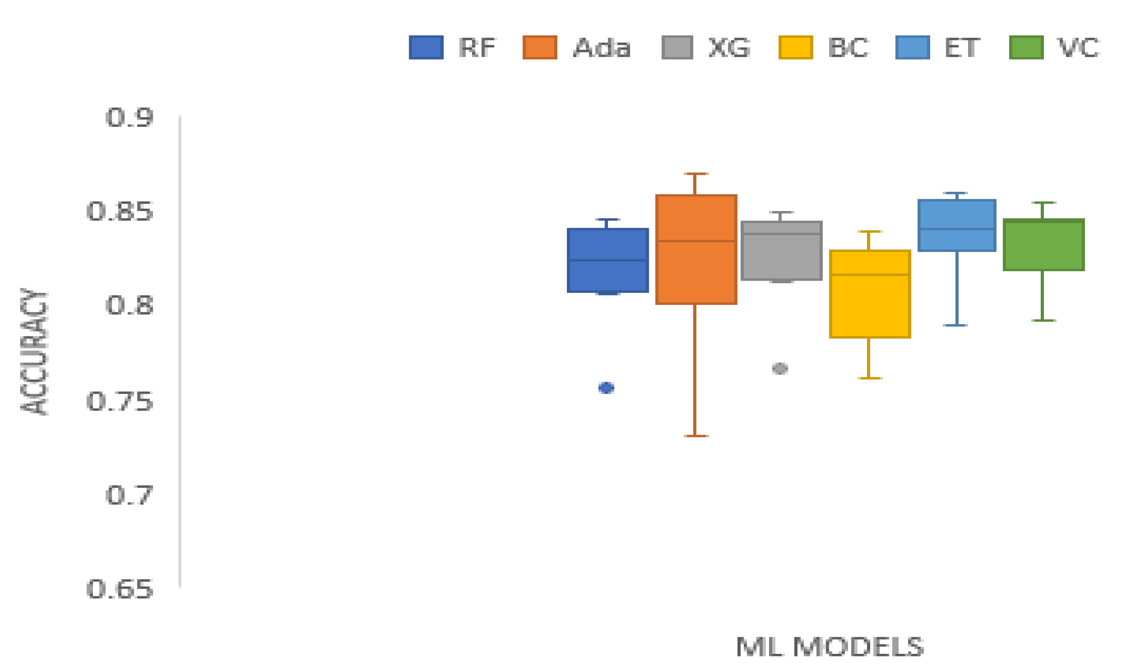
Table 3 shows the accuracy results of the tree-based ensemble ML models on the test datasets. The accuracy results of Random Forest range from 0.7565 to 0.8375. Adaboost has accuracy outcomes that range from 0.7306 to 0.8702. XGBoost accuracy scores range from 0.7667 to 0.8498. Bagging classifier accuracy results range from 0.7620 to 0.8391. The accuracy results of Extra Trees classifier range from 0.7889 to 0.8594. Voting Classifier accuracy results range from 0.7917 to 0.8552. AdaBoost produced the highest accuracy performance on XOM and TATASTEEL data sets. Extra Trees recorded the best accuracy performance on DJIA, and HCLTECH data sets. Voting classifier generated the best performance on MSFT, and KMX data sets. The Extra Trees classifier, and the Voting classifier produced the same and highest accuracy performance on BAC, and S&P_500 data sets. Overall, the Extra Trees classifier generated the best mean accuracy performance. Figure 2 provides the box plot of the accuracy scores of the machine learning models on the test data sets.
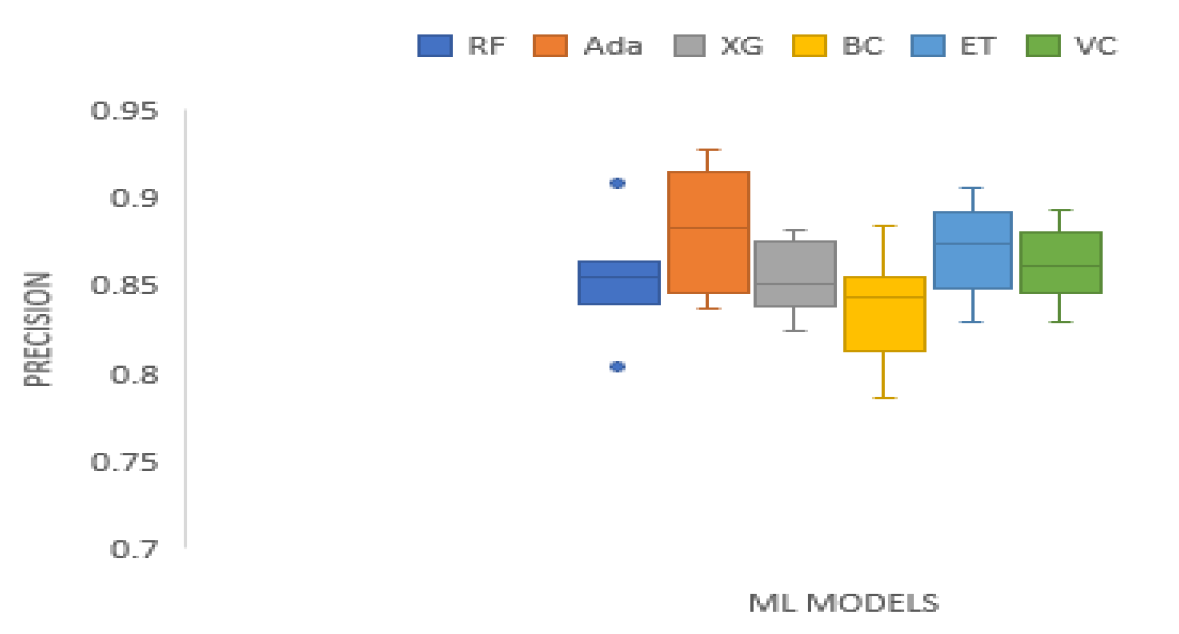
Table 4 displays precision results of the tree-based ensemble ML models on the test datasets. The precision scores of Random Forest range from 0.8033 to 0.9085. Adaboost precision scores range from 0.8372 to 0.9277. XGBoost has precision scores ranging from 0.8242 to 0.8822. Bagging Classifier precision results range from 0.7855 to 0.8841. The precision outcomes of Extra Trees range from 0.8298 to 0.9057. Voting Classifier precision scores range from 0.8297 to 0.8934. Random Forest recorded the best precision value on XOM data set. AdaBoost produced the highest precision values on S&P_500, MSFT, DJIA, and TATASTEEL datasets. Extra Trees generated the best precision scores on KMX, and HCLTECH data sets. On the whole, AdaBoost recorded the highest precision mean score. Figure 3 presents the boxplot of the precision results of the tree-based ensemble machine learning models on the test data sets.
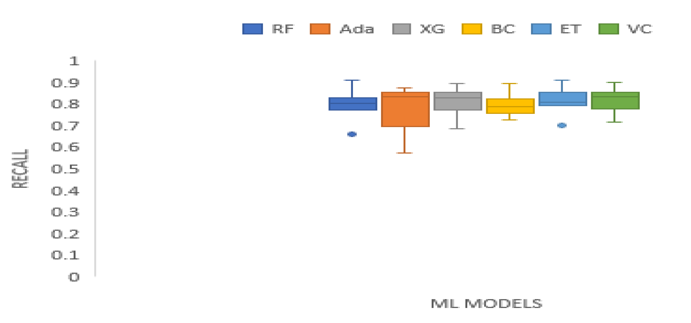
Table 5 presents recall outputs of the tree-based ensemble ML models on the test datasets. The recall outputs of Random Forest range from 0.6622 to 0.9089. Adaboost has recall scores that range from 0.5731 to 0.8750. The recall outcomes of XGBoost range from 0.6857 to 0.8940. Bagging Classifier has recall scores ranging from 0.7286 to 0.8962. Extra trees recall scores range from 0.7008 to 0.9089. The Voting Classifier has a recall results ranging from 0.7176 to 0.8983. Random Forest recorded the best recall value on TATASTEEL data set. AdaBoost produced the highest recall scores on BAC, and XOM data sets. XGBoost generated the best recall values on KMX, and HCLTECH data sets. The recall results generated by Bagging is the best on S&P_500, and KMX data sets. Extra Trees recorded the highest recall values on DJIA, and TATASTEEL. In general, the Voting Classifier produced the highest mean recall score. A boxplot illustrating the recall scores of the ensemble machine learning models on the test data sets is given by Figure 4.
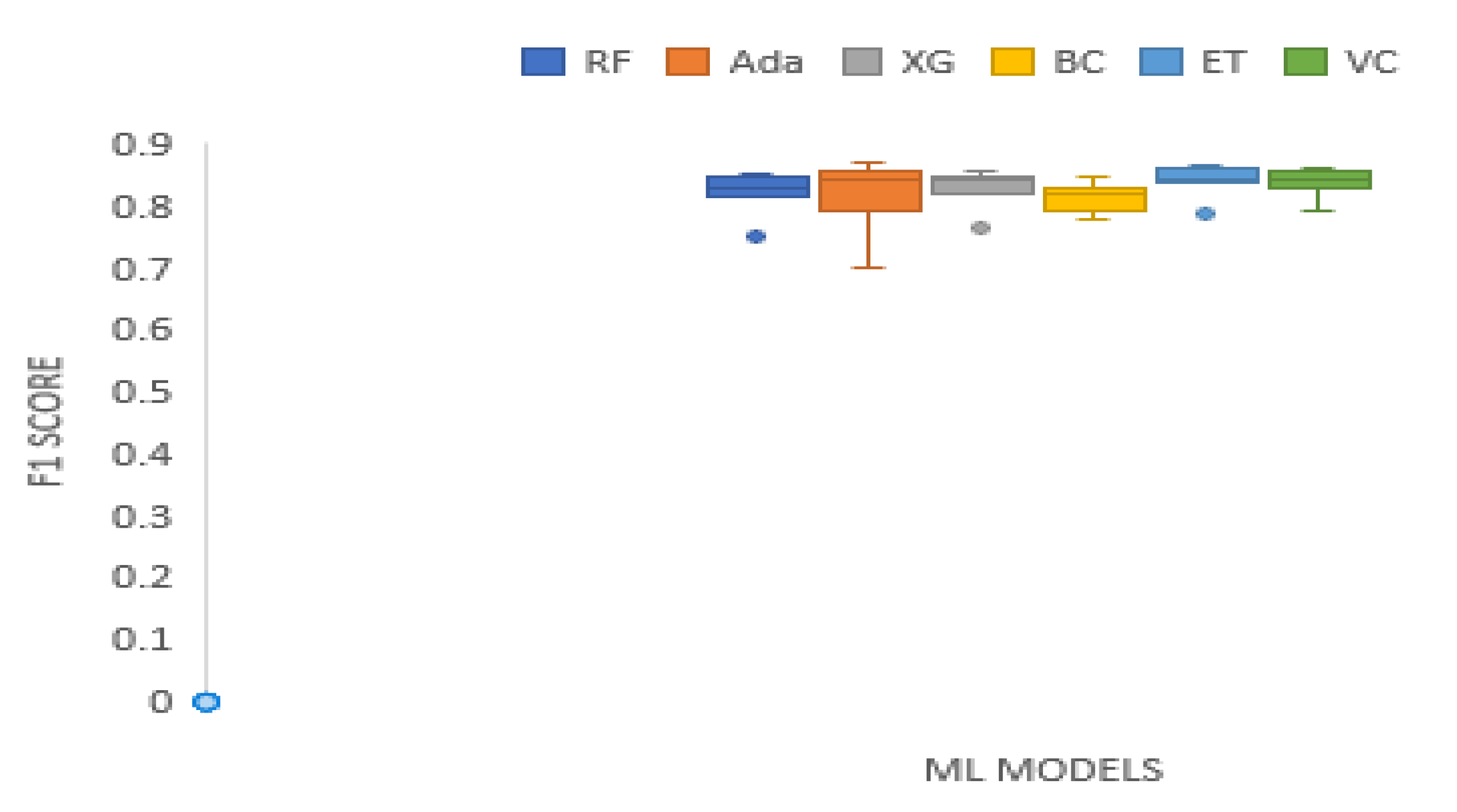
Table 6. shows F1 scores of the tree-based ensemble ML models on the test datasets. The F1 scores of Random range from 0.7498 to 0.8529. AdaBoost F1 results range from 0.7009 to 0.8722. XGBoost has F1 scores which range from 0.7640 to 0.8577. The F1 scores of Bagging Classifier range from 0.7803 to 0.8494. Extra Trees F1 scores range from 0.7853 to 0.8675. Voting Classifier has F1 score ranging from 0.7915 to 0.8627. AdaBoost generated the best F1 results on XOM, and TATSTEEL data sets. The Extra Trees classifier generated F1 results superior to the rest of the models on BAC, DJIA, and HCLTECH data set. The F1 values recorded by Voting Classifier is the highest on XOM, MSFT, and KMX data sets. Overall, the Extra Trees Classifier has the highest average F1score. A boxplot of the F1 scores of the tree-based ensemble machine learning models on the test data sets is illustrated by Figure 5.
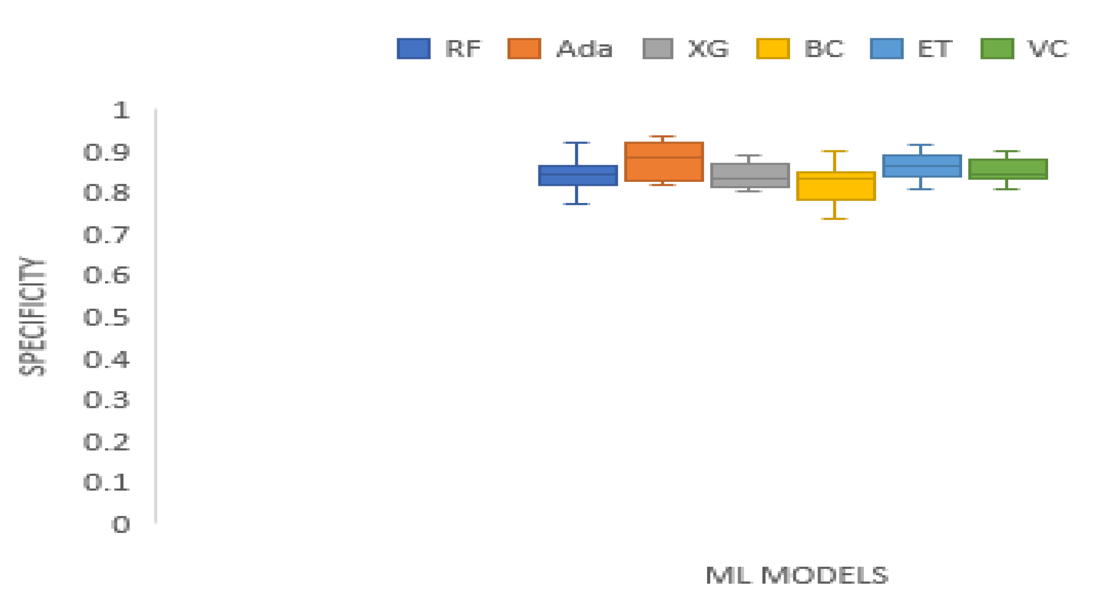
Table 7 presents specificity of the tree-based ensemble ML models on the test datasets. The specificity results of Random Forest range from 0.7717 to 0.9189. AdaBoost specificity scores range from 0.8194 to 0.9366. XGBoost has specificity scores ranging from 0.8043 to 0.8887. The specificity outcomes of Bagging Classifier range from 0.7381 to 0.8981. Extra trees specificity scores range from 0.8087 to 0.9132. Voting Classifier has specificity scores which range from 0.8109 to 0.9019. Random Forest generated the best specificity score on XOM data set. AdaBoost produced the highest specificity results on S&P_500, MSFT, DJIA, and TATSTEEL data sets. Bagging classifier recorded the best specificity performance on BAC data set. Extra Trees classifier generated the best specificity outcomes on KMX, and HCLTECH data sets. In general, AdaBoost classifier has the highest mean specificity score. Figure 6 presents the boxplot of the specificity scores of the tree-based ensemble machine learning models on the test data sets.
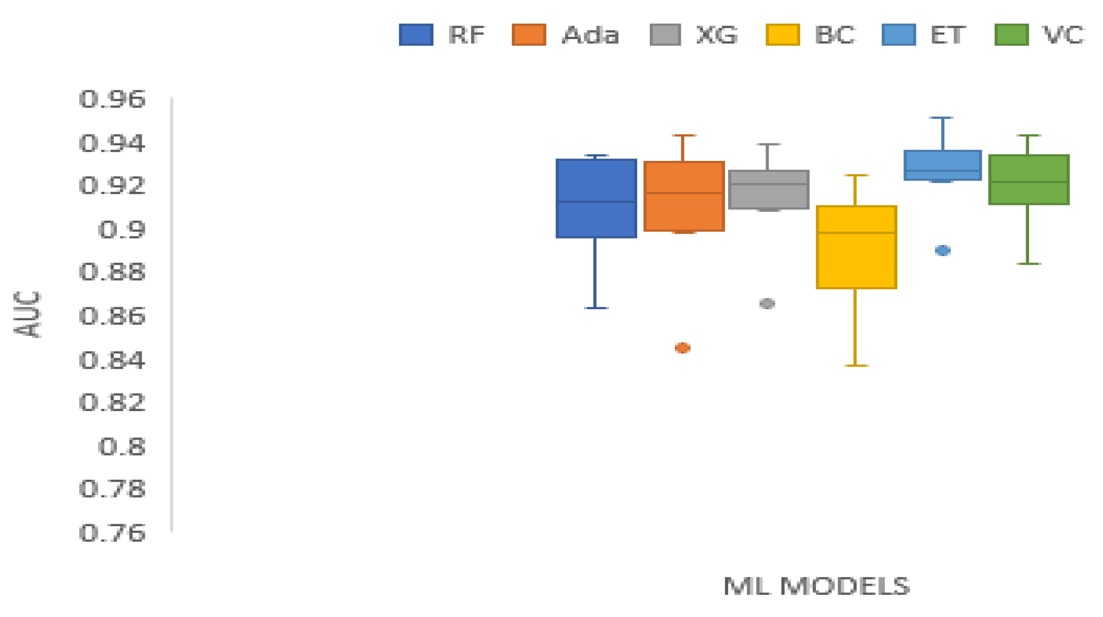
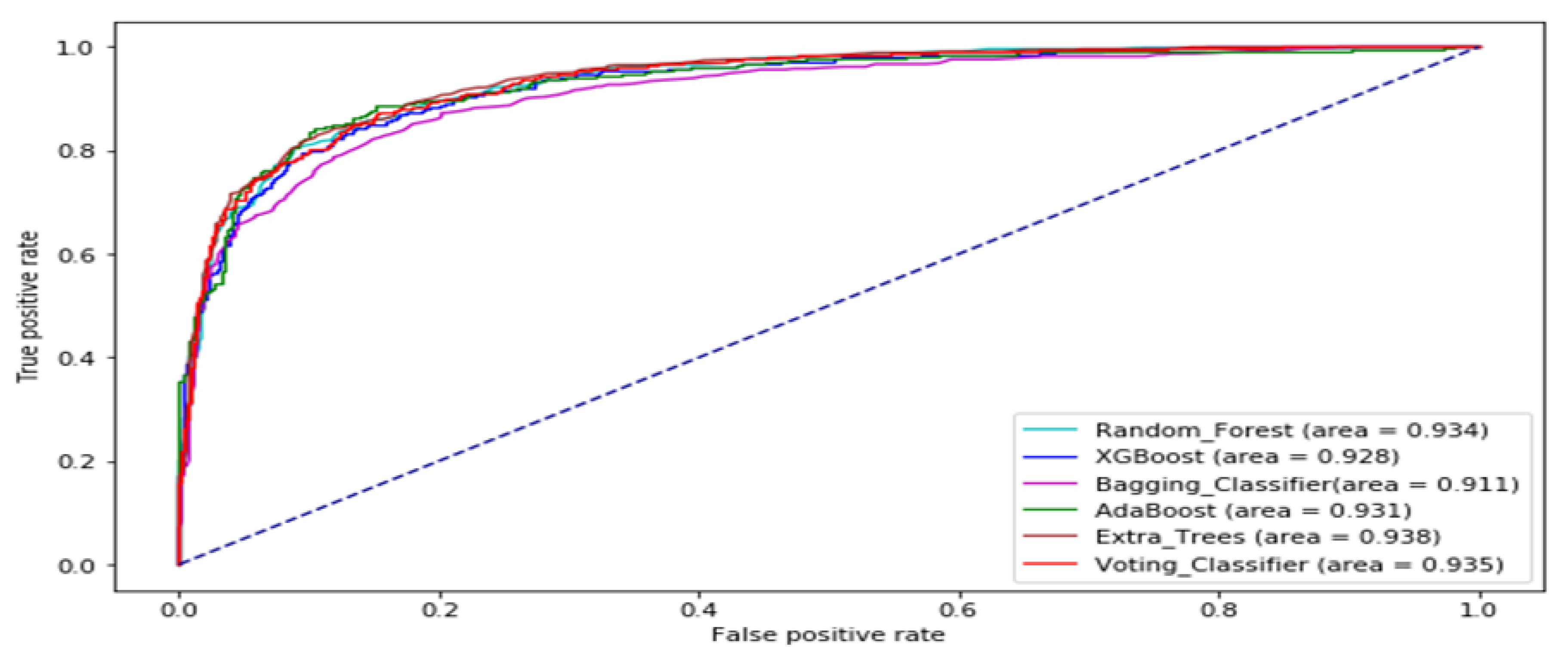
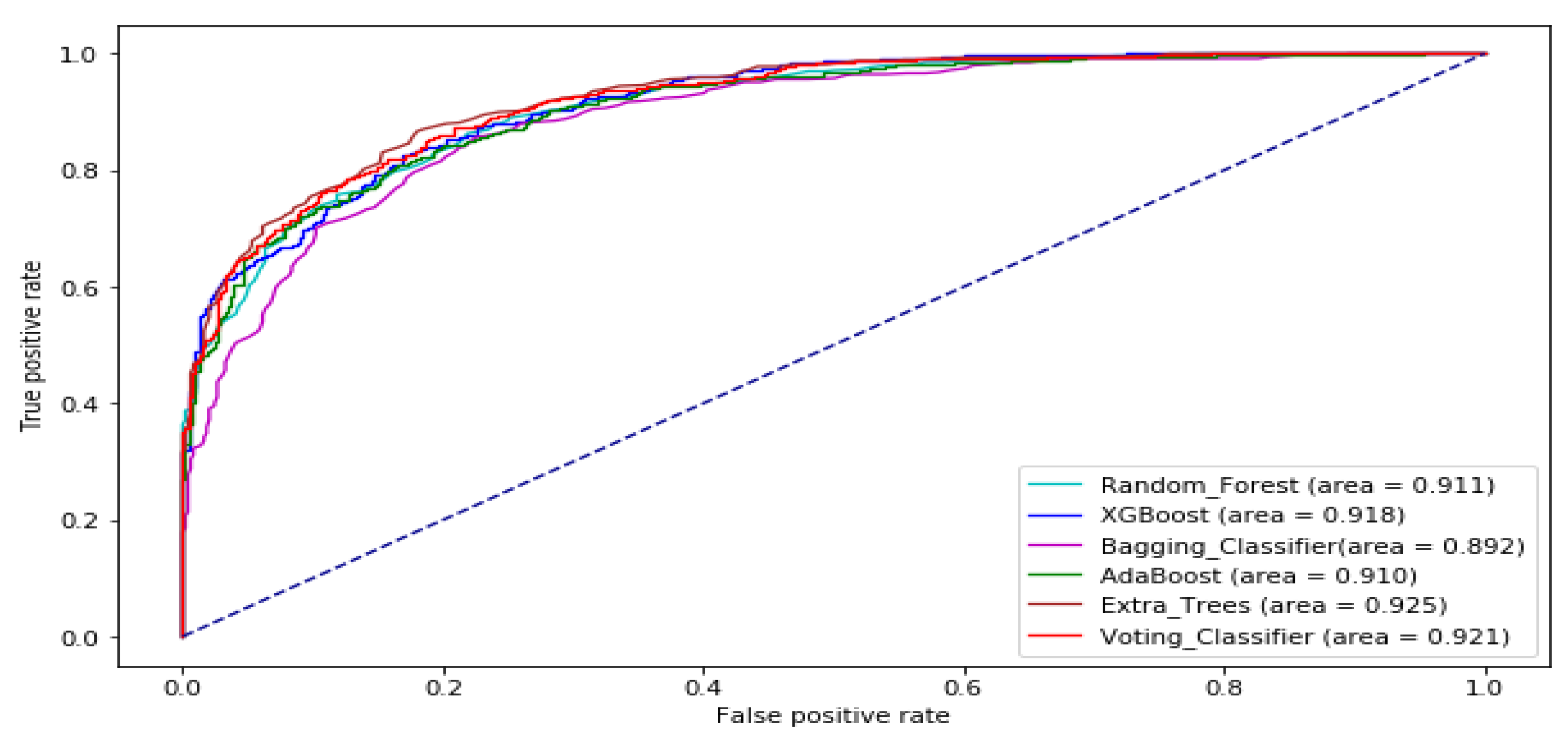
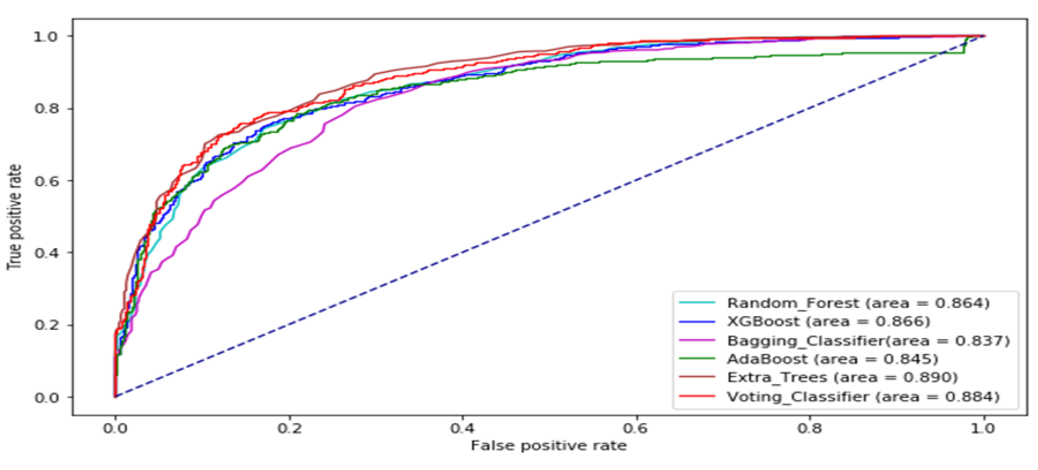
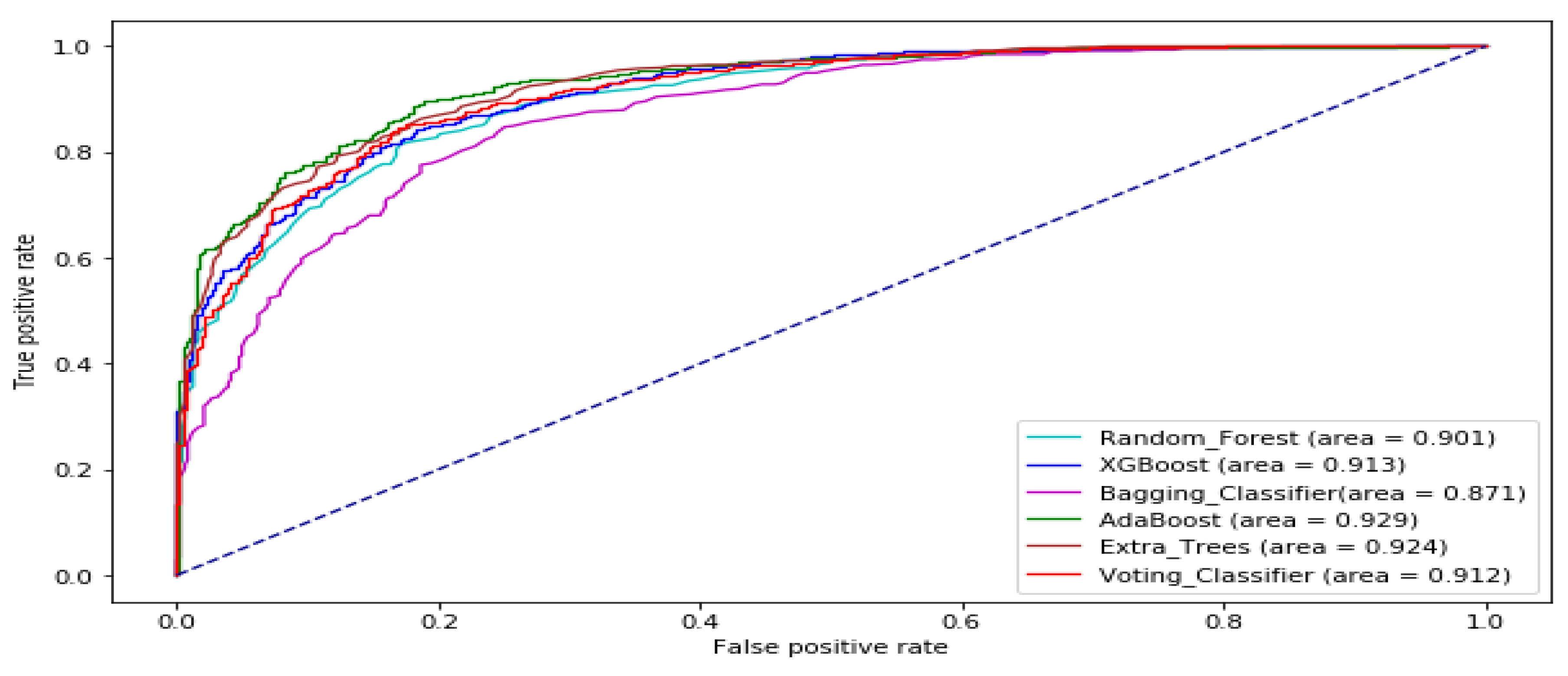
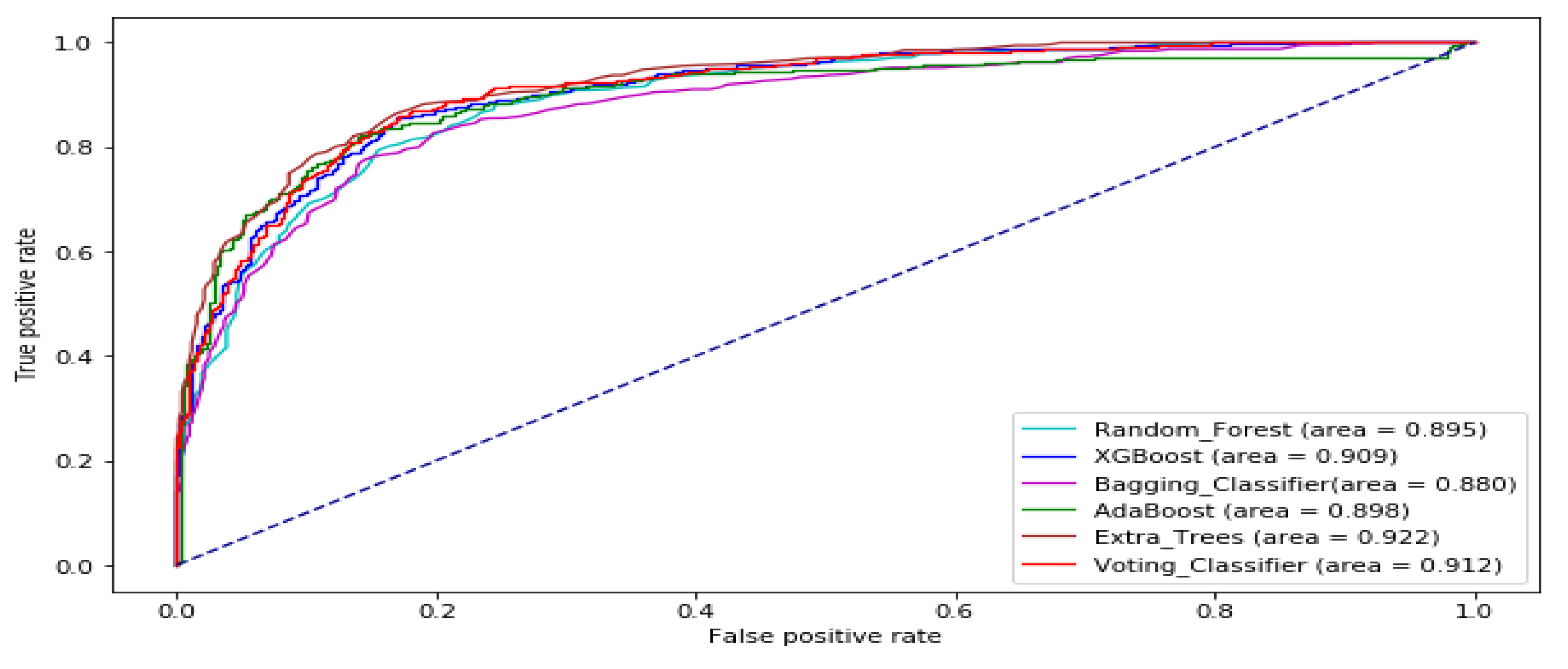
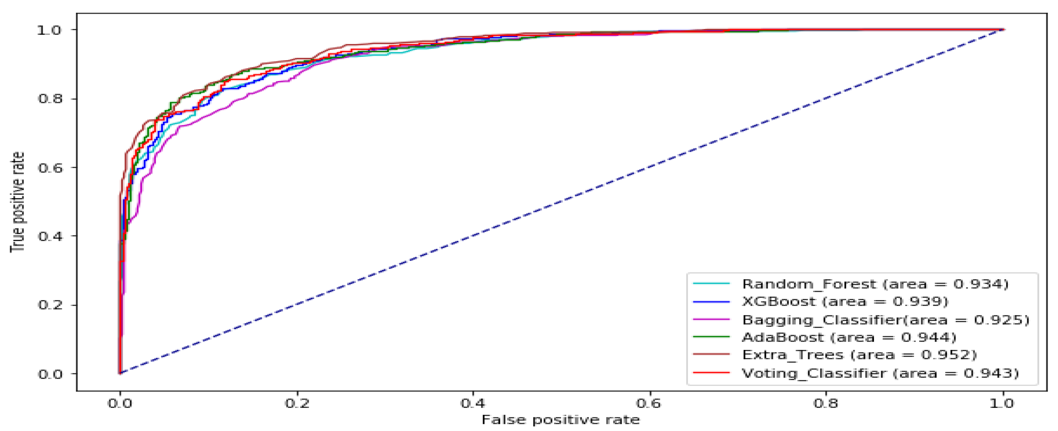
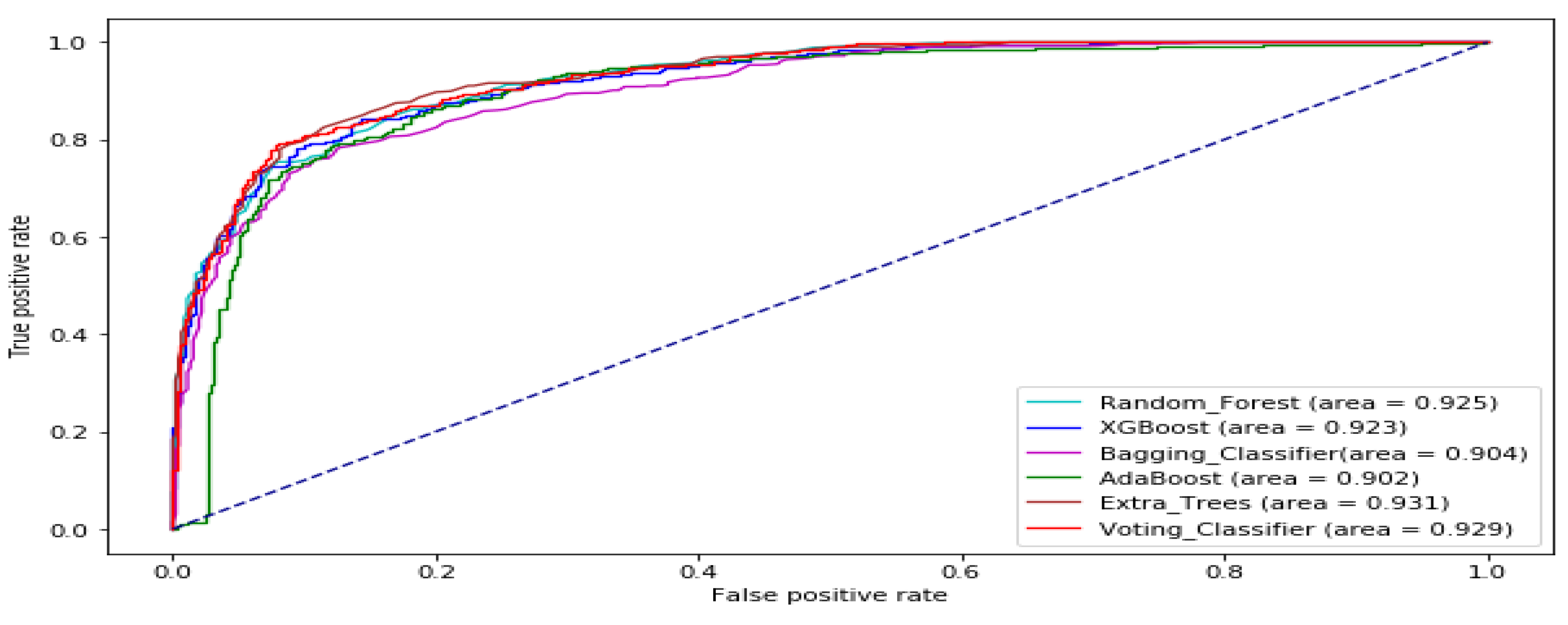
Table 8 displays AUC values of the tree-based ensemble ML models on the test datasets. The AUC values of Random Forest range from 0.8638 to 0.9340. AdaBoost has AUC values ranging from 0.8451 to 0.9436. XGBoost AUC values range from 0.8656 to 0.9392. Bagging Classifier has AUC scores ranging from 0.8366 to 0.9245. Extra trees AUC scores range from 0.8898 to 0.9515. The AUC results of Voting Classifier range from 0.8838 to 0.9428. AdaBoost generated the best AUC output on DJIA data set. The Extra Trees classifier produced the highest AUC values on BAC, XOM, S&P_500, MSFT, TATASTEEL, and HCLTECH data sets in Supplementary Materials. Overall, the Extra Trees classifier has the highest average AUC score. Figure 7 provides the boxplot of the AUC measure of the tree-based ensemble machine learning models on the test data sets.
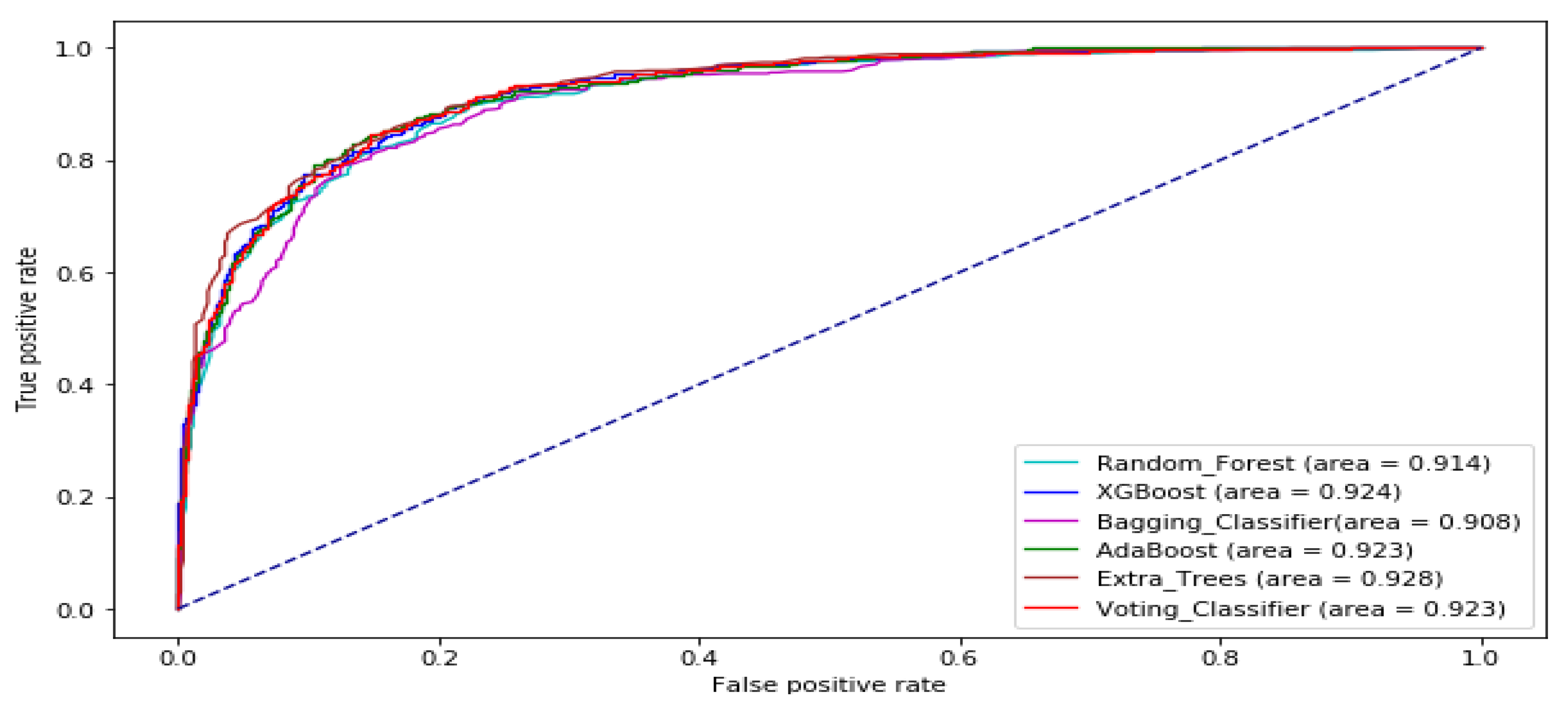
The ROC curve of all the tree-based ensemble ML on BAC, XOM, S&P 500, MSFT, DJIA, KMX, TATASTEEL, and HCLTECH stock datasets are displayed by Figure 8, Figure 9, Figure 10, Figure 11, Figure 12, Figure 13, Figure 14 and Figure 15 respectively. This presents a model with good separability and ROC curve passing close to the upper left corner.
A quantitative procedure utilizing Kendall W test of concordance is applied to rank the effectiveness of the tree-based ML algorithms in predicting the direction of stock price movement. In the study, we used a cut-off value of 0.05 for the significance level (p-value). We considered the Kendall’s coefficient significant and capable of giving an overall ranking when p < 0.05. The critical value for chi-square ( ) at p = 0.05 for five (5) degrees of freedom is 11.071. The degrees of freedom is equal to the total number of ML algorithms minus one. In this work, six ML algorithms are used giving us 5 degrees of freedom. Table 9 shows the results of Kendall’s W tests in using accuracy of the ten-fold cross validation on the training data sets. The outcomes of Kendall’s W tests in using accuracy, precision, recall, F1-measure, specificity, and AUC metrics on the test data sets are displayed by Table 10, Table 11, Table 12, Table 13, Table 14 and Table 15 below respectively.
Analysis of Table 9 indicates that Kendall’s coefficient using the accuracy of the ten-fold cross-validation on the training data set is significant (p < 0.05, > 11.071). The performance of AdaBoost classifier is superior the rest of the ensemble models. The overall ranking is AdaBoost > VC > ET > XGBoost > RF > BC.
Analysis of Table 10 shows that Kendall’s coefficient using the accuracy measure on the test data set is significant (p < 0.05, > 11.071). The performance of Extra Tree Classifier is superior to the rest of the ensemble models. The overall ranking is ET >VC > Adaboost > XGBoost > RF > BC.
Table 11. indicates that Kendall’s coefficient using the precision metric on the test data set is significant (p < 0.05, > 11.071). Extra Tree Classifier is the foremost performer among the ML ensemble models. The overall ranking is ET > AdaBoost > VC > RF > BC > XGBoost.
An analysis of Table 12 shows that Kendall’s coefficient using the recall metric on the test data set is not significant (p > 0.05, < 11.071), hence this measure cannot be used to rank the ML ensemble models.
Table 13 indicates that Kendall’s coefficient using the F1 score on the test data set is significant (p < 0.05, > 11.071) and that the performance of Extra Tree Classifier surpass that of the other ensemble ML models. The overall ranking is ET >VC > Adaboost = XGBoost > RF > BC.
Analysis of Table 14 demonstrates that Kendall’s coefficient test using the specificity metric on the test data set is not significant (p > 0.05, < 11.071), hence this measure cannot be used to rank the ML ensemble models.
Table 15 shows that Kendall’s coefficient using the AUC metric on the test data set is significant (p < 0.05, > 11.071) and that the performance of Extra Tree classifier is ranked the highest among the ensemble ML models. The overall ranking is ET >VC > XGBoost > Adaboost > RF > BC.
4. Conclusions
This paper evaluated and compared the effectiveness six different tree-based ensemble machine learning algorithms in predicting the direction of stock price movement. Stock data were randomly collected from three different stock exchanges. Each datum was split into two sets, the training set and the test set. The models were evaluated with ten-fold cross validation accuracy on the training set. In addition, the models were evaluated on the test set using accuracy, precision, recall, f1-score, specificity, and AUC metrics. The Kendall W test of concordance was adopted to rank the effectiveness of the tree-based ML algorithms. The experimental results indicated that for the ten-fold cross validation accuracy of the training set, the AdaBoost model outperformed the other models. For the test data, only accuracy, precision, f1-score, and AUC metrics were able to generate results significant to rank the different models using Kendall W test of concordance. The Extra Tree model performed better than the rest of the models on the test data set. A limitation of this study is that it considered only tree-based ensemble models. Hence, in our future work, we will incorporate machine learning models that involve the Gaussian process, a regularization technique, and kernel-based techniques.
Supplementary Materials
The BAC, XOM, KMX, S&P_500, DJIA, TATASTEEL, and HCLTECH stock data used are available online at https://www.mdpi.com/2078-2489/11/6/332/s1. All the data used for this work can also be obtained through Yahoo Finance API.
Author Contributions
E.K.A.: conceptualization, methodology, software, data curation, and Writing of original draft; Z.Q.: supervision, and resources; G.N.: data curation, and writing-reviewing and editing. All authors have read and agreed to the published version of the manuscript.
Funding
This work was supported by the NSFC-Guangdong Joint Fund (Grant No. U1401257), National Natural Science Foundation of China (Grant Nos. 61300090, 61133016, and 61272527), science and technology plan projects in Sichuan Province (Grant No. 2014JY0172) and the opening project of Guangdong Provincial Key Laboratory of Electronic Information Products Reliability Technology (Grant No. 2013A061401003).
Conflicts of Interest
The authors declare no conflict of interest.
Appendix A

Table A1.
Description of Overlap Studies Indicators used in the study.
| Overlap Studies Indicators | Description |
|---|---|
| Bollinger Bands (BBANDS) | Describes the different highs and lows of a financial instrument in a particular duration. |
| Weighted Moving Average (WMA) | Moving average that assign a greater weight to more recent data points than past data points |
| Exponential Moving Average (EMA) | Weighted moving average that puts greater weight and importance on current data points, however, the rate of decrease between a price and its preceding price is not consistent. |
| Double Exponential Moving Average (DEMA) | It is based on EMA and attempts to provide a smoothed average with less lag than EMA. |
| Kaufman Adaptive Moving Average (KAMA) | Moving average designed to be responsive to market trends and volatility. |
| MESA Adaptive Moving Average (MAMA) | Adjusts to movement in price based on the rate of change of phase as determined by the Hilbert transform discriminator. |
| Midpoint Price over period (MIDPRICE) | Average of the highest close minus lowest close within the look back period |
| Parabolic SAR (SAR) | Heights potential reversals in the direction of market price of securities. |
| Simple Moving Average (SMA) | Arithmetic moving average computed by averaging prices over a given time period. |
| Triple Exponential Moving Average (T3) | It is a triple smoothed combination of the DEMA and EMA |
| Triple Exponential Moving Average (TEMA) | An indicator used for smoothing price fluctuations and filtering out volatility. Provides a moving average having less lag than the classical exponential moving average. |
| Triangular Moving Average (TRIMA) | Moving average that is double smoothed (averaged twice) |
Table A2.
Description of Volume Indicators used in the study.
| Volume Indicator | Description |
|---|---|
| Chaikin A/D Line (ADL) | Estimates the Advance/Decline of the market. |
| Chaikin A/D Oscillator (ADOSC) | Indicator of another indicator. It is created through application of MACD to the Chaikin A/D Line |
| On Balance Volume (OBV) | Uses volume flow to forecast changes in price of stock |
Table A3.
Description of Price Transform Function Indicators.
| Price Transform Indicator | Description |
|---|---|
| Median Price (MEDPRICE) | Measures the mid-point of each day’s high and low prices. |
| Typical Price (TYPPRICE) | Measures the average of each day’s price. |
| Weighted Close Price (WCLPRICE) | Average of each day’s price with extra weight given to the closing price. |
Table A4.
Description of momentum indicators used in the study.
| Momentum Indicators | Description |
|---|---|
| Average Directional Movement Index (ADX) | Measures how strong or weak (strength of) a trend is over time |
| Average Directional Movement Index Rating (ADXR) | Estimates momentum change in ADX. |
| Absolute Price Oscillator (APO) | Computes the differences between two moving averages |
| Aroon | Used to find changes in trends in the price of an asset |
| Aroon Oscillator (AROONOSC) | Used to estimate the strength of a trend |
| Balance of Power (BOP) | Measures the strength of buyers and sellers in moving stock prices to the extremes |
| Commodity Channel Index (CCI) | Determine the price level now relative to an average price level over a period of time |
| Chande Momentum Oscillator (CMO) | Estimated by computing the difference between the sum of recent gains and the sum of recent losses |
| Directional Movement Index (DMI) | Indicate the direction of movement of the price of an asset |
| Moving Average Convergence/Divergence (MACD) | Uses moving averages to estimate the momentum of a security asset |
| Money Flow Index (MFI) | Utilize price and volume to identify buying and selling pressures |
| Minus Directional Indicator (MINUS_DI) | Component of ADX and it is used to identify presence of downtrend. |
| Momentum (MOM) | Measurement of price changes of a financial instrument over a period of time |
| Plus Directional Indicator (PLUS_DI) | Component of ADX and it is used to identify presence of uptrend. |
| Log Return | The log return for a period of time is the addition of the log returns of partitions of that period of time. It makes the assumption that returns are compounded continuously rather than across sub-periods |
| Percentage Price Oscillator (PPO) | Computes the difference between two moving averages as a percentage of the bigger moving average |
| Rate of change (ROC) | Measure of percentage change between the current price with respect to a at closing price n periods ago. |
| Relative Strength Index (RSI) | Determines the strength of current price in relation to preceding price |
| Stochastic (STOCH) | Measures momentum by comparing closing of a security with earlier trading range over a specific period of time |
| Stochastic Relative Strength Index (STOCHRSI) | Used to estimate whether a security is overbought or oversold. It measures RSI over its own high/low range over a specified period. |
| Ultimate Oscillator (ULTOSC) | Estimates the price momentum of a security asset across different time frames. |
| Williams’ %R (WILLR) | Indicates the position of the last closing price relative to the highest and lowest price over a time period. |
References
- Fischer, T.; Krauss, C. Deep learning with long short-term memory networks for financial market predictions. Eur. J. Oper. Res. 2018, 270, 654–669. [Google Scholar] [CrossRef] [Green Version]
- Cootner, P. The Random Character of Stock Market Prices; M.I.T. Press: Cambridge, MA, USA, 1964. [Google Scholar]
- Fama, E.F.; Fisher, L.; Jensen, M.C.; Roll, R. The adjustment of stock prices to new information. Int. Econ. Rev. 1969, 10, 1–21. [Google Scholar] [CrossRef]
- Malkiel, B.G.; Fama, E.F. Efficient capital markets: A review of theory and empirical work. J. Financ. 1970, 25, 383–417. [Google Scholar] [CrossRef]
- Fama, E.F. The behavior of stock-market prices. J. Bus. 1965, 38, 34–105. [Google Scholar] [CrossRef]
- Jensen, M.C. Some anomalous evidence regarding market efficiency. J. Financ. Econ. 1978, 6, 95–101. [Google Scholar] [CrossRef]
- Bollen, J.; Mao, H.; Zeng, X. Twitter mood predicts the stock market. J. Comput. Sci. 2011, 2, 1–8. [Google Scholar] [CrossRef] [Green Version]
- Ballings, M.; Van den Poel, D.; Hespeels, N.; Gryp, R. Evaluating multiple classifiers for stock price direction prediction. Expert Syst. Appl. 2015, 42, 7046–7056. [Google Scholar] [CrossRef]
- Chong, E.; Han, C.; Park, F.C. Deep learning networks for stock market analysis and prediction: Methodology, data representations, and case studies. Expert Syst. Appl. 2017, 83, 187–205. [Google Scholar] [CrossRef] [Green Version]
- Nofsinger, J.R. Social mood and financial economics. J. Behav. Financ. 2005, 6, 144–160. [Google Scholar] [CrossRef]
- Smith, V.L. Constructivist and ecological rationality in economics. Am. Econ. Rev. 2003, 93, 465–508. [Google Scholar] [CrossRef]
- Avery, C.N.; Chevalier, J.A.; Zeckhauser, R.J. The CAPS prediction system and stock market returns. Rev. Financ. 2016, 20, 1363–1381. [Google Scholar] [CrossRef] [Green Version]
- Hsu, M.-W.; Lessmann, S.; Sung, M.-C.; Ma, T.; Johnson, J.E. Bridging the di- vide in financial market forecasting: Machine learners vs. financial economists. Expert Syst. Appl. 2016, 61, 215–234. [Google Scholar] [CrossRef] [Green Version]
- Weng, B.; Ahmed, M.A.; Megahed, F.M. Stock market one-day ahead movement prediction using disparate data sources. Expert Syst. Appl. 2017, 79, 153–163. [Google Scholar] [CrossRef]
- Zhang, Y.; Wu, L. Stock market prediction of s&p 500 via combination of improved bco approach and bp neural network. Expert Syst. Appl. 2009, 36, 8849–8854. [Google Scholar]
- Patel, J.; Shah, S.; Thakkar, P.; Kotecha, K. Predicting stock market index using fusion of machine learning techniques. Expert Syst. Appl. 2015, 42, 2162–2172. [Google Scholar] [CrossRef]
- Geva, T.; Zahavi, J. Empirical evaluation of an automated intraday stock recommendation system incorporating both market data and textual news. Decis. Support Syst. 2014, 57, 212–223. [Google Scholar] [CrossRef]
- Guresen, E.; Kayakutlu, G.; Daim, T.U. Using artificial neural network models in stock market index prediction. Expert Syst. Appl. 2011, 38, 10389–10397. [Google Scholar] [CrossRef]
- Meesad, P.; Rasel, R.I. Predicting stock market price using support vector regression. In Proceedings of the 2013 International Conference on Informatics, Electronics and Vision (ICIEV), Dhaka, Bangladesh, 17–18 May 2013; pp. 1–6. [Google Scholar]
- Wang, J.-Z.; Wang, J.-J.; Zhang, Z.-G.; Guo, S.-P. Forecasting stock indices with back propagation neural network. Expert Syst. Appl. 2011, 38, 14346–14355. [Google Scholar] [CrossRef]
- Schumaker, R.P.; Chen, H. Textual analysis of stock market prediction us- ing breaking financial news: The azfin text system. ACM Trans. Inf. Syst. 2009, 27, 12. [Google Scholar] [CrossRef]
- Barak, S.; Modarres, M. Developing an approach to evaluate stocks by fore- casting effective features with data mining methods. Expert Syst. Appl. 2015, 42, 1325–1339. [Google Scholar] [CrossRef]
- Booth, A.; Gerding, E.; Mcgroarty, F. Automated trading with performance weighted random forests and seasonality. Expert Syst. Appl. 2014, 41, 3651–3661. [Google Scholar] [CrossRef]
- Chen, Y.; Yang, B.; Abraham, A. Flexible neural trees ensemble for stock index modeling. Neurocomputing 2007, 70, 697–703. [Google Scholar] [CrossRef]
- Hassan, M.R.; Nath, B.; Kirley, M. A fusion model of hmm, ann and ga for stock market forecasting. Expert Syst. Appl. 2007, 33, 171–180. [Google Scholar] [CrossRef]
- Rather, A.M.; Agarwal, A.; Sastry, V. Recurrent neural network and a hybrid model for prediction of stock returns. Expert Syst. Appl. 2015, 42, 3234–3241. [Google Scholar] [CrossRef]
- Wang, L.; Zeng, Y.; Chen, T. Back propagation neural network with adaptive differential evolution algorithm for time series forecasting. Expert Syst. Appl. 2015, 42, 855–863. [Google Scholar] [CrossRef]
- Qian, B.; Rasheed, K. Stock market prediction with multiple classifiers. Appl. Intell. 2007, 26, 25–33. [Google Scholar] [CrossRef]
- Xiao, Y.; Xiao, J.; Lu, F.; Wang, S. Ensemble ANNs-PSO-GA approach for day-ahead stock E-exchange prices forecasting. Int. J. Comput. Intell. Syst. 2014, 7, 272–290. [Google Scholar] [CrossRef] [Green Version]
- Mohamad, I.B.; Usman, D. Standardization and Its Effects on K-Means Clustering Algorithm. Res. J. Appl. Sci. Eng. Technol. 2013, 6, 3299–3303. [Google Scholar] [CrossRef]
- Lin, X.; Yang, Z.; Song, Y. Short-term stock price prediction based on echo state networks. Expert Syst. Appl. 2009, 36, 7313–7317. [Google Scholar] [CrossRef]
- Tsai, C.-F.; Hsiao, Y.-C. Combining multiple feature selection methods for stock prediction: Union, intersection, and multi-intersection approaches. Decis. Support Syst. 2010, 50, 258–269. [Google Scholar] [CrossRef]
- Torlay, L.; Perrone-Bertolotti, M.; Thomas, E. Machine learning–XGBoost analysis of language networks to classify patients with epilepsy. Brain Inform. 2017, 4, 159–169. [Google Scholar] [CrossRef] [PubMed]
- Breiman, L. Random forests. Mach. Learn. 2001, 45, 5–32. [Google Scholar] [CrossRef] [Green Version]
- Ho, T.K. Random decision forests. In Document Analysis and Recognition, Proceedings of the Third International Conference, Montreal, QC, Canada, 14–16 August 1995; IEEE: New York, NY, USA, 1995; Volume 1, pp. 278–282. [Google Scholar]
- Ho, T.K. The random subspace method for constructing decision forests. Intell. IEEE Trans. Pattern Anal. Mach. 1998, 20, 832–844. [Google Scholar]
- Amit, Y.; Geman, D. Shape quantization and recognition with randomized trees. Neural Comput. 1997, 9, 1545–1588. [Google Scholar] [CrossRef] [Green Version]
- Breiman, L. Bagging predictors. Mach. Learn. 1996, 24, 123–140. [Google Scholar] [CrossRef] [Green Version]
- Boinee, P.; De Angelis, A.; Foresti, G.L. Meta random forests. Int. J. Comput. Intell. 2005, 2, 138–147. [Google Scholar]
- Zhou, Y.; Qiu, G. Random forest for label ranking. Expert Syst. Appl. 2018, 112, 99–109. [Google Scholar] [CrossRef] [Green Version]
- Tan, Z.; Yan, Z.; Zhu, G. Stock selection with random forest: An exploitation of excess return in the Chinese stock market. Heliyon 2019, 5, e02310. [Google Scholar] [CrossRef] [Green Version]
- Chen, M.; Wang, X.; Feng, B.; Liu, W. Structured random forest for label distribution learning. Neurocomputing 2018, 320, 171–182. [Google Scholar] [CrossRef]
- Wongvibulsin, S.; Wu, K.C.; Zeger, S.L. Clinical risk prediction with random forests for survival, longitudinal, and multivariate (RF-SLAM) data analysis. BMC Med Res. Methodol. 2020, 20, 1. [Google Scholar] [CrossRef] [Green Version]
- Seifert, S. Application of random forest-based approaches to surface-enhanced Raman scattering data. Sci. Rep. 2020, 10, 5436. [Google Scholar] [CrossRef] [PubMed]
- Freund, Y.; Schapire, R. Experiments with a new boosting algorithm. In Machine Learning: Proceedings of the Thirteenth International Conference (ICML ’96); Morgan Kaufmann Publishers Inc.: Bari, Italy, 1996; pp. 148–156. [Google Scholar]
- Friedman, J.; Hastie, T.; Tibshirani, R. Additive logistic regression: A 723 statistical view of boosting. Ann. Stat. 2000, 28, 337–374. [Google Scholar] [CrossRef]
- Wang, J.; Tang, S. Time series classification based on Arima and AdaBoost, 2019 International Conference on Computer Science Communication and Network Security (CSCNS2019). MATEC Web Conf. 2020, 309, 03024. [Google Scholar] [CrossRef] [Green Version]
- Chang, V.; Li, T.; Zeng, Z. Towards an improved AdaBoost algorithmic method for computational financial analysis. J. Parallel Distrib. Comput. 2019, 134, 219–232. [Google Scholar] [CrossRef]
- Suganya, E.; Rajan, C. An AdaBoost-modified classifier using stochastic diffusion search model for data optimization in Internet of Things. Soft Comput. 2019, 1–11. [Google Scholar] [CrossRef]
- Friedman, J.H. Greedy function approximation: A gradient boosting machine. Ann. Stat. 2001, 29, 1189–1232. [Google Scholar] [CrossRef]
- Chen, T.; Guestrin, C. Xgboost: A scalable tree boosting system. In Proceedings of the 22nd ACM SIGKDD International Conference on Knowledge Discovery and Data Mining (KDD ’16), San Francisco, CA, USA, 13–17 August 2016; pp. 785–794. [Google Scholar]
- Liang, W.; Luo, S.; Zhao, G.; Wu, H. Predicting hard rock pillar stability using GBDT, XGBoost, and LightGBM Algorithms. Mathematics 2020, 8, 765. [Google Scholar] [CrossRef]
- Li, W.; Yin, Y.; Quan, X.; Zhang, H. Gene expression value prediction based on XGBoost algorithm. Front. Genet. 2019, 10, 1077. [Google Scholar] [CrossRef] [Green Version]
- Sharma, A.; Verbeke, W.J.M.I. Improving Diagnosis of Depression with XGBOOST Machine Learning Model and a Large Biomarkers Dutch Dataset (n = 11,081). Front. Big Data 2020, 3, 15. [Google Scholar] [CrossRef]
- Zareapoora, M.; Shamsolmoali, P. Application of Credit Card Fraud Detection: Based on Bagging Ensemble Classifier. Int. Conf. Intell. Comput. Commun. Converg. Procedia Comput. Sci. 2015, 48, 679–686. [Google Scholar] [CrossRef] [Green Version]
- Yaman, E.; Subasi, A. Comparison of Bagging and Boosting Ensemble Machine Learning Methods for Automated EMG Signal Classification. Biomed Res. Int. 2019, 2019, 13. [Google Scholar] [CrossRef] [PubMed]
- Roshan, S.E.; Asadi, S. Improvement of Bagging performance for classification of imbalanced datasets using evolutionary multi-objective optimization. Eng. Appl. Artif. Intell. 2020, 87, 103319. [Google Scholar] [CrossRef]
- Geurts, P.; Ernst, D.; Wehenkel, L. Extremely randomized trees. Mach. Learn. 2006, 63, 3–42. [Google Scholar] [CrossRef] [Green Version]
- Zafari, A.; Zurita-Milla, R.; Izquierdo-Verdiguier, E. Land Cover Classification Using Extremely Randomized Trees: A Kernel Perspective. IEEE Geosci. Remote Sens. Lett. 2019, 1–5. [Google Scholar] [CrossRef]
- Sharma, J.; Giri, C.; Granmo, O.C.; Goodwin, M. Multi-layer intrusion detection system with ExtraTrees feature selection, extreme learning machine ensemble, and softmax aggregation. EURASIP J. Info. Secur. 2019, 2019, 15. [Google Scholar] [CrossRef] [Green Version]
Figure 1.
Boxplot of ten-fold cross validation accuracy scores of the tree-based ensemble ML models on the training data sets.
Figure 1.
Boxplot of ten-fold cross validation accuracy scores of the tree-based ensemble ML models on the training data sets.

Figure 2.
Boxplot of accuracy scores of the tree-based ensemble ML models on the test data sets.

Figure 3.
Boxplot of precision results of the tree-based ensemble ML models on the test data sets.

Figure 4.
Boxplot of recall scores of the tree-based ensemble ML models on the test data sets.

Figure 5.
Boxplot of F1 scores of the tree-based ensemble ML models on the test data.

Figure 6.
Boxplot of specificity scores of the tree-based ensemble ML models on the test data sets.

Figure 7.
Boxplot of AUC measure of the tree-based ensemble ML models on the test data sets.

Figure 8.
ROC Curve of tree-based ensemble Machine Learning models on BAC test dataset.

Figure 9.
ROC Curve of tree-based ensemble Machine Learning models on XOM test data set.

Figure 10.
ROC Curve of tree-based ensemble Machine Learning models on S&P_500 test data set.

Figure 11.
ROC Curve of tree-based ensemble Machine Learning models on MSFT test data set.

Figure 12.
ROC Curve of tree-based ensemble Machine Learning models on DJIA test data set.

Figure 13.
ROC Curve of tree-based ensemble Machine Learning models on KMX test data set.

Figure 14.
ROC Curve of tree-based ensemble Machine Learning models on TATASTEEL test data set.

Figure 15.
ROC Curve of tree-based ensemble Machine Learning models on HCLTECH test data set.

Table 1.
Description of the data sets.
| Data Set | Stock Market | Time Frame | Number of Sample |
|---|---|---|---|
| BAC | NYSE | 2005-01-01 to 2019-12-30 | 3774 |
| DOWJONES | INDEXDJX | 2005-01-01 to 2019-12-30 | 3774 |
| TATASTEEL | NSE | 2005-01-01 to 2019-12-30 | 3279 |
| HCLTECH | NSE | 2005-01-01 to 2019-12-30 | 3477 |
| KMX | NYSE | 2005-01-01 to 2019-12-30 | 3774 |
| MSFT | NASDAQ | 2005-01-01 to 2019-12-30 | 3774 |
| S&P_500 | INDEXSP | 2005-01-01 to 2019-12-30 | 3774 |
| XOM | NYSE | 2005-01-01 to 2019-12-30 | 3774 |
Table 2.
Ten-fold cross validation accuracy score of the ML models on the training sets.
| Data Sets | RF | Ada | XG | BC | ET | VC |
|---|---|---|---|---|---|---|
| BAC | 0.8345 | 0.8452 | 0.8392 | 0.8277 | 0.8329 | 0.8444 |
| XOM | 0.8181 | 0.8157 | 0.8249 | 0.8034 | 0.8170 | 0.8269 |
| S&P 500 | 0.8766 | 0.9004 | 0.8909 | 0.8607 | 0.8972 | 0.8960 |
| MSFT | 0.8388 | 0.8476 | 0.8478 | 0.8234 | 0.8531 | 0.8503 |
| DJIA | 0.8884 | 0.9127 | 0.8991 | 0.8781 | 0.9027 | 0.9019 |
| KMX | 0.8483 | 0.8626 | 0.8480 | 0.8273 | 0.8551 | 0.8519 |
| TATASTEEL | 0.8679 | 0.8720 | 0.8679 | 0.8472 | 0.8716 | 0.8674 |
| HCLTECH | 0.8131 | 0.8282 | 0.8122 | 0.8092 | 0.8087 | 0.8191 |
| Mean | 0.8482 | 0.8606 | 0.8538 | 0.8346 | 0.8547 | 0.8572 |
Table 3.
Accuracy outputs of the tree-based ensemble ML models on the test datasets.
| Data Sets | RF | Ada | XG | BC | ET | VC |
|---|---|---|---|---|---|---|
| BAC | 0.8306 | 0.8435 | 0.8417 | 0.8306 | 0.8463 | 0.8463 |
| XOM | 0.8463 | 0.8639 | 0.8454 | 0.8222 | 0.8574 | 0.8463 |
| S&P 500 | 0.8139 | 0.7926 | 0.8213 | 0.8120 | 0.8287 | 0.8287 |
| MSFT | 0.7565 | 0.7306 | 0.7667 | 0.7620 | 0.7889 | 0.7917 |
| DJIA | 0.8055 | 0.8278 | 0.8120 | 0.7731 | 0.8306 | 0.8148 |
| KMX | 0.8185 | 0.8361 | 0.8407 | 0.8138 | 0.8361 | 0.8426 |
| TATASTEEL | 0.8412 | 0.8702 | 0.8498 | 0.8391 | 0.8594 | 0.8552 |
| HCLTECH | 0.8375 | 0.8335 | 0.8355 | 0.8184 | 0.8527 | 0.8456 |
| Mean | 0.8188 | 0.8248 | 0.8266 | 0.8089 | 0.8375 | 0.8344 |
Table 4.
Precision results of the tree-based ensemble ML models on the test datasets.
| Data Sets | RF | Ada | XG | BC | ET | VC |
|---|---|---|---|---|---|---|
| BAC | 0.8392 | 0.8372 | 0.8378 | 0.8469 | 0.8429 | 0.8491 |
| XOM | 0.9085 | 0.8959 | 0.8822 | 0.8841 | 0.9057 | 0.8934 |
| S&P 500 | 0.8421 | 0.9277 | 0.8592 | 0.8311 | 0.8664 | 0.8612 |
| MSFT | 0.8640 | 0.9021 | 0.8626 | 0.7855 | 0.8929 | 0.8822 |
| DJIA | 0.8630 | 0.9185 | 0.8803 | 0.8398 | 0.8891 | 0.8767 |
| KMX | 0.8457 | 0.8448 | 0.8389 | 0.8469 | 0.8687 | 0.8442 |
| TATASTEEL | 0.8033 | 0.8695 | 0.8242 | 0.8073 | 0.8298 | 0.8297 |
| HCLTECH | 0.8629 | 0.8470 | 0.8438 | 0.8577 | 0.8796 | 0.8623 |
| Mean | 0.8536 | 0.8803 | 0.8536 | 0.8374 | 0.8719 | 0.8624 |
Table 5.
Recall measure of the tree-based ensemble ML models on the test datasets.
| Data Set | RF | Ada | XG | BC | ET | VC |
|---|---|---|---|---|---|---|
| BAC | 0.8255 | 0.8600 | 0.8545 | 0.8145 | 0.8582 | 0.8491 |
| XOM | 0.7764 | 0.8291 | 0.8036 | 0.7491 | 0.8036 | 0.7927 |
| S&P 500 | 0.8122 | 0.6734 | 0.8054 | 0.8240 | 0.8122 | 0.8190 |
| MSFT | 0.6622 | 0.5731 | 0.6857 | 0.7815 | 0.7008 | 0.7176 |
| DJIA | 0.7705 | 0.7554 | 0.7638 | 0.7286 | 0.7923 | 0.7739 |
| KMX | 0.7943 | 0.8372 | 0.8569 | 0.7818 | 0.8050 | 0.8533 |
| TATASTEEL | 0.9089 | 0.8750 | 0.8940 | 0.8962 | 0.9089 | 0.8983 |
| HCLTECH | 0.8324 | 0.8454 | 0.8547 | 0.7970 | 0.8436 | 0.8510 |
| Mean | 0.7978 | 0.7811 | 0.81488 | 0.7966 | 0.8156 | 0.8194 |
Table 6.
F1 scores of the tree-based ensemble ML models on the test datasets.
| Data Set | RF | Ada | XG | BC | ET | VC |
|---|---|---|---|---|---|---|
| BAC | 0.8323 | 0.8484 | 0.8461 | 0.8304 | 0.8505 | 0.8491 |
| XOM | 0.8373 | 0.8612 | 0.8411 | 0.8110 | 0.8516 | 0.8401 |
| S&P 500 | 0.8269 | 0.7804 | 0.8314 | 0.8275 | 0.8384 | 0.8395 |
| MSFT | 0.7498 | 0.7009 | 0.7640 | 0.7834 | 0.7853 | 0.7915 |
| DJIA | 0.8142 | 0.8290 | 0.8179 | 0.7803 | 0.8379 | 0.8221 |
| KMX | 0.8192 | 0.8410 | 0.8478 | 0.8130 | 0.8357 | 0.8488 |
| TATASTEEL | 0.8529 | 0.8722 | 0.8577 | 0.8494 | 0.8675 | 0.8627 |
| HCLTECH | 0.8474 | 0.8462 | 0.8492 | 0.8263 | 0.8612 | 0.8566 |
| Mean | 0.8225 | 0.8224 | 0.8319 | 0.8152 | 0.8410 | 0.8388 |
Table 7.
Specificity scores of the tree-based ensemble ML models on the test datasets.
| Data Set | RF | Ada | XG | BC | ET | VC |
|---|---|---|---|---|---|---|
| AC | 0.8358 | 0.8264 | 0.8283 | 0.8472 | 0.8340 | 0.8440 |
| XOM | 0.9189 | 0.9000 | 0.8887 | 0.8981 | 0.9132 | 0.9019 |
| S&P 500 | 0.8160 | 0.9366 | 0.8405 | 0.7975 | 0.8487 | 0.8405 |
| MSFT | 0.8722 | 0.9237 | 0.8660 | 0.7381 | 0.8969 | 0.8825 |
| DJIA | 0.8489 | 0.9172 | 0.8716 | 0.8282 | 0.8778 | 0.8654 |
| KMX | 0.8445 | 0.8349 | 0.8234 | 0.8484 | 0.8695 | 0.8311 |
| TATASTEEL | 0.7717 | 0.8652 | 0.8043 | 0.7804 | 0.8087 | 0.8109 |
| HCLTECH | 0.8436 | 0.8194 | 0.8128 | 0.8436 | 0.8634 | 0.8392 |
| Mean | 0.8440 | 0.8779 | 0.8420 | 0.8227 | 0.8640 | 0.8519 |
Table 8.
AUC of the tree-based ensemble ML models on the test dataset.
| DataSet | RF | Ada | XG | BC | ET | VC |
|---|---|---|---|---|---|---|
| BAC | 0.9143 | 0.9230 | 0.9241 | 0.9081 | 0.9280 | 0.9231 |
| XOM | 0.9340 | 0.9314 | 0.9283 | 0.9112 | 0.9378 | 0.9351 |
| S&P 500 | 0.9109 | 0.9099 | 0.9176 | 0.8921 | 0.9250 | 0.9207 |
| MSFT | 0.8638 | 0.8451 | 0.8656 | 0.8366 | 0.8898 | 0.8838 |
| DJIA | 0.9014 | 0.9294 | 0.9133 | 0.8706 | 0.9243 | 0.9123 |
| KMX | 0.8950 | 0.8979 | 0.9087 | 0.8802 | 0.9219 | 0.9116 |
| TATASTEEL | 0.9335 | 0.9436 | 0.9392 | 0.9245 | 0.9515 | 0.9428 |
| HCLTECH | 0.9254 | 0.9023 | 0.9232 | 0.9042 | 0.9306 | 0.9293 |
| Mean | 0.9098 | 0.9103 | 0.9150 | 0.8909 | 0.9261 | 0.9198 |
Table 9.
Rankings of Tree-Based Machine Learning Ensemble models based on Kendall W Test results using accuracy measure of ten-fold cross validation on the training data set.
Table 9.
Rankings of Tree-Based Machine Learning Ensemble models based on Kendall W Test results using accuracy measure of ten-fold cross validation on the training data set.
| Measure | W | p | Ranks | |||||||
|---|---|---|---|---|---|---|---|---|---|---|
| Accuracy | 0.5496 | 21.9821 | 0.0005 | Technique | RF | Ada | XG | BC | ET | VC |
| Mean Rank | 2.9375 | 5.1250 | 3.4375 | 1.125 | 4.0000 | 4.3750 |
Table 10.
Rankings of Tree-Based Machine Learning Ensemble models based on Kendall W Test results using accuracy metric on the test data set.
Table 10.
Rankings of Tree-Based Machine Learning Ensemble models based on Kendall W Test results using accuracy metric on the test data set.
| Measure | W | p | Ranks | |||||||
|---|---|---|---|---|---|---|---|---|---|---|
| Accuracy | 0.5821 | 23.2857 | 0.0003 | Technique | RF | Ada | XG | BC | ET | VC |
| Mean Rank | 2.5000 | 3.5625 | 3.3750 | 1.4375 | 5.1875 | 4.9375 |
Table 11.
Rankings of Tree-Based Machine Learning Ensemble models based on Kendall W Test results using precision metric on the test data set.
Table 11.
Rankings of Tree-Based Machine Learning Ensemble models based on Kendall W Test results using precision metric on the test data set.
| Measure | W | p | Ranks | |||||||
|---|---|---|---|---|---|---|---|---|---|---|
| Precision | 0.3554 | 14.2143 | 0.0143 | Technique | RF | Ada | XG | BC | ET | VC |
| Mean Rank | 3.2500 | 4.2500 | 2.1250 | 2.5000 | 5.1250 | 3.7500 |
Table 12.
Rankings of Tree-Based Machine Learning Ensemble models based on Kendall W Test results using recall metric on the test data set.
Table 12.
Rankings of Tree-Based Machine Learning Ensemble models based on Kendall W Test results using recall metric on the test data set.
| Measure | W | p | Ranks | |||||||
|---|---|---|---|---|---|---|---|---|---|---|
| Recall | 0.1746 | 6.9821 | 0.2220 | Technique | RF | Ada | XG | BC | ET | VC |
| Mean Rank | 2.8750 | 3.1250 | 3.8125 | 2.5000 | 4.3125 | 4.3750 |
Table 13.
Rankings of Tree-Based Machine Learning Ensemble models based on Kendall W Test results using F1 score on the test data set.
Table 13.
Rankings of Tree-Based Machine Learning Ensemble models based on Kendall W Test results using F1 score on the test data set.
| Measure | W | p | Ranks | |||||||
|---|---|---|---|---|---|---|---|---|---|---|
| F1 Score | 0.5696 | 22.7857 | 0.0004 | Technique | RF | Ada | XG | BC | ET | VC |
| Mean Rank | 2.1250 | 3.6250 | 3.6250 | 1.6250 | 5.1250 | 4.8750 |
Table 14.
Rankings of Tree-Based Machine Learning Ensemble models based on Kendall W Test results using Specificity metric on the test data set.
Table 14.
Rankings of Tree-Based Machine Learning Ensemble models based on Kendall W Test results using Specificity metric on the test data set.
| Measure | W | p | Ranks | |||||||
|---|---|---|---|---|---|---|---|---|---|---|
| Specificity | 0.2598 | 10.3929 | 0.0648 | Technique | RF | Ada | XG | BC | ET | VC |
| Mean Rank | 3.3125 | 4.1250 | 2.1875 | 2.8125 | 4.8750 | 3.6875 |
Table 15.
Rankings of Tree-Based Machine Learning Ensemble models based on Kendall W Test results using AUC metric on the test data set.
Table 15.
Rankings of Tree-Based Machine Learning Ensemble models based on Kendall W Test results using AUC metric on the test data set.
| Measure | W | p | Ranks | |||||||
|---|---|---|---|---|---|---|---|---|---|---|
| AUC | 0.7429 | 29.7143 | 0.0000 | Technique | RF | Ada | XG | BC | ET | VC |
| Mean Rank | 2.7500 | 3.1250 | 3.6250 | 1.1250 | 5.8750 | 4.5000 |
© 2020 by the authors. Licensee MDPI, Basel, Switzerland. This article is an open access article distributed under the terms and conditions of the Creative Commons Attribution (CC BY) license (http://creativecommons.org/licenses/by/4.0/).
Share and Cite
MDPI and ACS Style
Ampomah, E.K.; Qin, Z.; Nyame, G. Evaluation of Tree-Based Ensemble Machine Learning Models in Predicting Stock Price Direction of Movement. Information 2020, 11, 332. https://0-doi-org.brum.beds.ac.uk/10.3390/info11060332
AMA Style
Ampomah EK, Qin Z, Nyame G. Evaluation of Tree-Based Ensemble Machine Learning Models in Predicting Stock Price Direction of Movement. Information. 2020; 11(6):332. https://0-doi-org.brum.beds.ac.uk/10.3390/info11060332
Chicago/Turabian StyleAmpomah, Ernest Kwame, Zhiguang Qin, and Gabriel Nyame. 2020. "Evaluation of Tree-Based Ensemble Machine Learning Models in Predicting Stock Price Direction of Movement" Information 11, no. 6: 332. https://0-doi-org.brum.beds.ac.uk/10.3390/info11060332
Note that from the first issue of 2016, this journal uses article numbers instead of page numbers. See further details here.