Dimensionality Reduction for Human Activity Recognition Using Google Colab


Center for Distributed and Mobile Computing, EECS, University of Cincinnati, Cincinnati, OH 45221, USA
*
Author to whom correspondence should be addressed.
Information 2021, 12(1), 6; https://0-doi-org.brum.beds.ac.uk/10.3390/info12010006
Submission received: 29 November 2020
/
Revised: 20 December 2020
/
Accepted: 20 December 2020
/
Published: 23 December 2020
(This article belongs to the Special Issue Recent Advances in IoT and Cyber/Physical Security)
Abstract
:Human activity recognition (HAR) is a classification task that involves predicting the movement of a person based on sensor data. As we can see, there has been a huge growth and development of smartphones over the last 10–15 years—they could be used as a medium of mobile sensing to recognize human activity. Nowadays, deep learning methods are in a great demand and we could use those methods to recognize human activity. A great way is to build a convolutional neural network (CNN). HAR using Smartphone dataset has been widely used by researchers to develop machine learning models to recognize human activity. The dataset has two parts: training and testing. In this paper, we propose a hybrid approach to analyze and recognize human activity on the same dataset using deep learning method on cloud-based platform. We have applied principal component analysis on the dataset to get the most important features. Next, we have executed the experiment for all the features as well as the top 48, 92, 138, and 164 features. We have run all the experiments on Google Colab. In the experiment, for the evaluation of our proposed methodology, datasets are split into two different ratios such as 70–10–20% and 80–10–10% for training, validation, and testing, respectively. We have set the performance of CNN (70% training–10% validation–20% testing) with 48 features as a benchmark for our work. In this work, we have achieved maximum accuracy of 98.70% with CNN. On the other hand, we have obtained 96.36% accuracy with the top 92 features of the dataset. We can see from the experimental results that if we could select the features properly then not only could the accuracy be improved but also the training and testing time of the model.
1. Introduction
Human activity recognition (HAR) is the process by which we could identify what a person is doing based on sensor readings. Generally, activities are divided into classes. The main goal of HAR is to identify which class of activity is being performed by the individuals. HAR has different applications in our life. For example, a HAR system could detect if there is any abnormal activity in a crowd of people. After that, it could allow identification of possible threatening situations or detect that a person is in need of assistance. Another scenario where identifying human activity could be very useful is the monitoring of elderly people in need of care [1]. Additionally, it could be useful in the field of interactive robotics (human–robot collaboration) and for assistive robotics [2,3].
With the daily usage of the smartphone, the embedded sensors such as accelerometer and gyroscope typically produce a huge amount of data, which are very useful. They can be used to predict and classify human activities automatically. Potentially, HAR can play an important role in elderly houses [4] especially in the countries where the average old population is on the rise. Similarly, the moves of a sports player [5] can be analyzed with its help. As a result, a player’s performance can be improved. Additionally, HAR based on sensors can play a vital role in Internet of Things (IoT) based technologies [6]. It has the potential to be utilized in a wide spectrum of applications, and consequently, it is an active topic of research. Many breakthroughs have been achieved in this area in the last few decades [7].
Additionally, HAR plays crucial role in the mental and physical wellbeing of the population [8]. Physicians could potentially manage patients’ diseases such as obesity, diabetes, and cardiovascular automatically by recognizing and monitoring their daily activities [9]. As a part of the treatment, these patients are usually required to follow an active exercise routine [10]. Patients can manage their lifestyle with the help of activity recognition system, and it will empower their physicians to properly monitor them and hence, offer appropriate recommendations. If the activities of the patients are monitored continuously then it will definitely help in reducing the hospital stay, improving reliability of diagnosis, and equally enhance patients’ quality of life [11]. Alford [12] argued that “apart from not smoking, being physically active is the most powerful lifestyle choice an individual can make for improved health outcomes” [8].
If we have a high dimensional dataset then it could potentially increase the learning time as well as the processing complexity. To address the problem, several studies have explored principal component analysis (PCA) as a preprocessing step in the deep learning framework. Kwak et al. [13] have shown the Effect of the Principal Component Analysis in Convolutional Neural Network for Hyperspectral Image Classification (HSIC). First, they applied PCA to the dataset to achieve dimensionality reduction. After that, they used the compressed dataset to train the CNN model. Additionally, they have analyzed the effect of PCA in deep learning for HSIC. Their results show that they have got very good efficiency by using reduced dimensions with the explained variance ratio of 99.7~99.8% [13].
In this paper, we have collected the dataset from Kaggle [14], which is a public repository. The dataset is named University of California Irvine (UCI) human activity recognition (HAR) using Smartphone. It is taken from J. L. Reyes-Ortiz et al. [15] and has been used in several projects [16,17,18]. The size of the dataset is 64.34 MB, and it has 10,299 instances in total.
Because we have high dimensional data with 561 features for HAR, it could also increase the learning time and processing complexity. In our work, we have transformed the dataset through PCA and applied into the CNN model by varying the size of the reduced dimensionality. At the same time, we have shown the impact of dimensionality reduction using PCA in deep learning networks for HAR.
Here, we have adopted a cloud-based platform, Google Colab to recognize human activity. We can process the dataset in real-time with the platform. We could analyze and visualize the data. Not only that but also, we can import a dataset, train the classifier on it, and evaluate the model. Colab notebooks run code on cloud servers from Google. It means that regardless of our machine’s capacity, we can harness the power of Google hardware, including graphics processing units (GPUs) and tensor processing units (TPUs). To perform all those things, only a simple browser is needed [19].
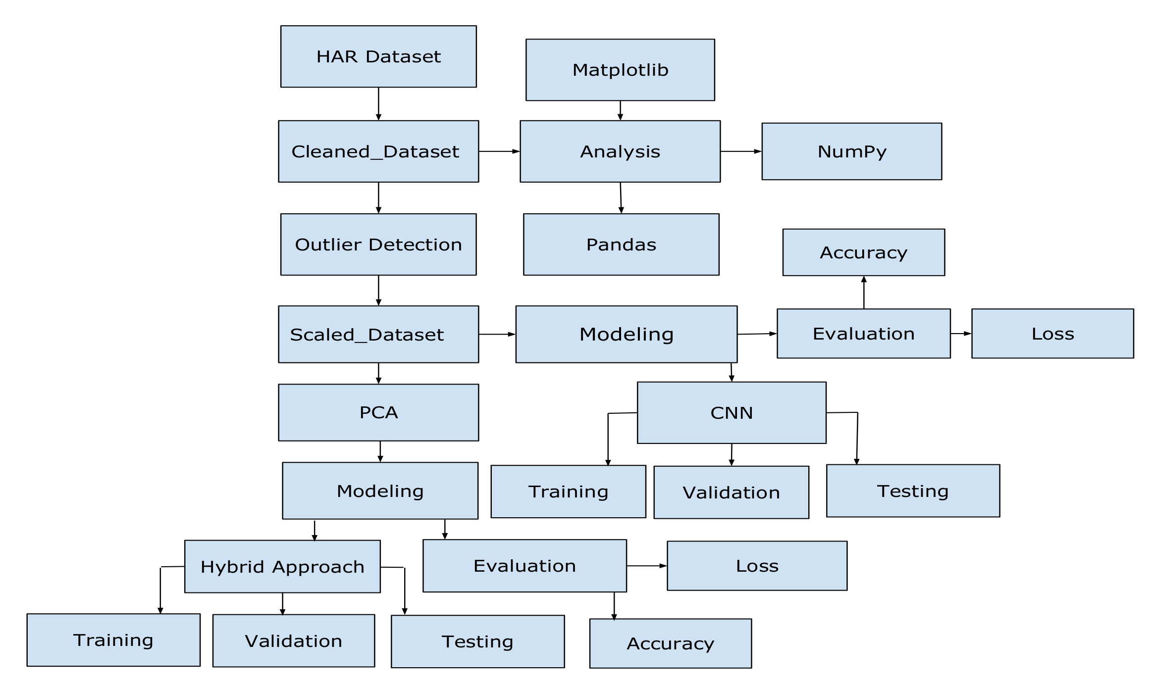
At the beginning, we have read the dataset and analyzed it so that we can understand all the features properly and figure out how they are related to each other [20]. Then, we clean the dataset for the experiment. Next, we have applied local outlier function to find out if there is any outlier in the dataset. After that, we have scaled the dataset using Robust Scaler since it has outliers. In the next step, we have applied PCA to get the most important features of the dataset to model our data. Additionally, we have considered deep learning method named convolutional neural network (CNN). After that, we have incorporated important features to our model. We have trained the model by using 70% (80%) of the dataset, kept 10% (10%) of the dataset for the validation and then tested it with the rest of the 20% (10%) of the dataset. We have run the experiments for all the features as well as top features of the dataset. We also made a comparison of the performance for all the features with the top features. Finally, it is shown that we could achieve good accuracy by using the top 92 features of the dataset with our hybrid approach.
The following are some of the key contributions and findings of our work: (1) We propose a method to analyze and recognize human activity on the same dataset using hybrid approach on cloud-based platform. (2) We have applied Local Outlier Function on the training part as well as the entire part of the dataset to find the outlier. After finding outliers in the dataset, we have used Robust Scaling method to scale the dataset. (3) We have applied PCA on the dataset to find the most important features to model our data. (4) We have achieved good accuracy compared to others only using the top features of the dataset. (5) Furthermore, we have improved the training time and testing time of the model.
The following describes the organization of the paper: we talk about problem statement in Section 2, Section 3 discusses the related work, Section 4 presents the proposed methodology, Section 5 explains the data analysis, Section 6 details the experiment with the implementation of the model, Section 7 demonstrates the implementation details with the results, and Section 8 concludes the study.
2. Problem Statement
All features do not contribute equally to predicting a disease or classifying the activities. If we include all the features of the dataset then it will become multi-dimensional and suffer from overfitting. Therefore, it is necessary that we apply feature selection technique to identity the important features and avoid the overfitting problem. Additionally, it is important that the learning algorithm only focus on the subset of features that are relevant and ignore the irrelevant features. That particular learning algorithm will be working on the training part of the dataset for selecting the best performing feature subset. After that, it could be applied to the testing part of the dataset. In this study, we apply dimensionality reduction technique to reduce the dimensions of the original feature space and achieve good classification results [21].
We know that healthcare systems are looking forward to offering better treatments to their patients. And they are trying to do that by monitoring the health of the patients in real-time constantly. Therefore, it is very important to have a system that could monitor the status of people with underlying health conditions and recognize the user activities right at home, which in turn will reduce patient’s unnecessary visits to the clinics. In this case, it is necessary that activities are recognized with minimal response time. Not only that but also if there are any abnormal activities tracked, it could notify the emergency department that the patient is in need of immediate care. In this situation, it is crucial that the right individuals are notified without any delays.
3. Related Work
Ullah et al. [7] have proposed an approach based on stacked long short-term memory (LSTM) network to recognize six human behaviors using smartphone data. The network consists of five LSTM cells, which are trained on the sensor data. A single layer neural network which preprocesses the data for the stacked LSTM network is followed by the network. They have used an L2 regularizer in the cost function to help in generalizing the network. After that, the network is evaluated on the UCI dataset and quantitative results are compared. They have measured the performance of the proposed approach in terms of precision, recall, and the average accuracy. Compared to the closest state-of-the-art method, the proposed approach has improved the average accuracy by 0.93 percent without doing any manual feature engineering.
Ogbuabor et al. [8] have analyzed the role of accelerometer and gyroscope sensor in activity recognition. In this work, they have used Multi-Layer Perceptron (MLP), which is widely used artificial neural networks for classification and prediction task. Their experimental results on HAR dataset [14,15] indicates that each of the sensors could be used for human activity recognition separately. However, the performance of accelerometer sensor data is better than gyroscope sensor data, and it has classification accuracy of 92%. They have concluded that the combination of accelerometer and gyroscope performed better than using them individually with an accuracy of 95%.
Sikder et al. [22] have described a multichannel CNN-based HAR classification model. First, they have extracted the frequency and power information from the signals. After that, they have fed them to a multichannel CNN model. Finally, the model is tested on the UCI HAR dataset [15], and their results show that they have achieved 95.25% classification accuracy.
Gaur et al. [23] have presented a framework for HAR using Apache Spark. They have used different classifiers such as logistic regression, DT, RF and logistic regression with cross-fold validation model to recognize the activities of humans. They have observed that the most convenient setup to deal with a variety of data is to use 70% of the dataset for training and 30% of the dataset for testing. Their results show that logistic regression with cross fold validated over 5-fold, have achieved better performance than other classifiers in terms of accuracy and F1-score. They have achieved accuracy score as high as 91.02% after testing over KAGGLE-UCI Human Activity Recognition Accelerometer-Sensor time series data [14].
Su et al. [24] have proposed an automated human activity recognition network HDL with smartphone motion sensor units. It is a multimodel fusion network. The proposed network is the combination of DBLSTM (deep bidirectional long short-term memory) model and CNN model. The experimental results show that they have obtained maximum accuracy of 97.95% with the proposed HDL network. They have used the updated version of the dataset, which has 10,929 instances in total [25,26]. For this reason, we will not compare our results with this work.
4. Proposed Methodology
In this section, we introduce our methodology as shown in Figure 1. First, we downloaded the dataset from public repository Kaggle [14], then uploaded it to Google Colab for our work, and cleaned it for our model. Figure 1 summarizes the steps that have been followed in this work.
4.1. Dataset Information
The dataset that has been used in this work [14,15] was collected by using a Samsung Galaxy S2. A group of 30 volunteers have participated in the experiment and their age range is 19–48 years. The smartphone was attached to the waist of each volunteer. Accelerometers and gyroscopes were used to record the data. The subjects performed six typical daily activities such as WALKING, WALKING_UPSTAIRS, WALKING_DOWNSTAIRS, SITTING, STANDING, and LAYING. By using its embedded sensors, 3-axial linear acceleration and 3-axial angular velocity were captured. The sampling rate that was used is 50Hz. Noise filters were applied to preprocess the sensor signals. After that, the acceleration signal was separated in its gravitational and body motion component. By using a sliding window filter, the measurements were filtered.
Finally, we have 561 features in total to use in this research with the combined data of accelerometer and gyroscope [1,8]. It comprises the time and frequency domain features of the sensor dataset. The dataset [14,15] contains 10,299 samples, which are separated into two sets (i.e., a training set and a test set). The former one contains 7352 samples (71.39%), whereas the latter one is comprised of the rest of the 2947 samples (28.61%). We have merged the training and testing sets to make it one single dataset.
Attribute Information: For each record in the dataset, it is provided with the information such as (1) triaxial acceleration from the accelerometer (total acceleration) and the estimated body acceleration, (2) triaxial angular velocity from the gyroscope, (3) a 561-feature vector, (4) its activity label, which is “target value”, and (5) an identifier of the subject who carried out the experiment.
4.2. Data Cleaning
Datasets that are available on the internet have some weaknesses such as many missing values and do not cover most of the aspects that the researchers are looking for. Therefore, in this case, the first thing we have to do is to clean the dataset to be good fit for the work. Additionally, we have deleted the unnecessary column that we do not need them such as Subject ID.
A dataset can contain extreme values that differ significantly from other data points and fall outside the expected range—they are known as outliers. In order to improve ML modeling, we can understand and even remove these outlier values [27].
We have used Isolation Forest, which is an unsupervised learning algorithm, for the outlier detection [28]. Instead of profiling normal data points, it explicitly identifies the anomalies. It is built on the basis of decision trees. It also can be scaled up and handle large, high-dimensional datasets [29].
We have got 368 outliers and 6984 inliers using Isolation Forest for the training part of the original dataset. Additionally, it detected 515 outliers and 9784 inliers for the entire dataset.
We need to scale our data, but because of the outliers, the standardization of the input variables is not easy. It can be achieved by ignoring the outliers from the calculation of the mean and standard deviation. Later, the calculated values could be used to scale the variable. This procedure is known as robust data scaling. It could be achieved by calculating the median (50th percentile) and the 25th and 75th percentiles. In the next step, the values of each variable have their median subtracted and are divided by the interquartile range (IQR), which is the difference between the 75th and 25th percentiles.
value = (value − median)/(p75 − p25)
The resulting variable will not be skewed by outliers. It will have a zero mean and median and a standard deviation of 1 [30].
For our work, we have used Robust Scaling technique to scale the numerical input variables. Because we have categorical values in the activity column, label encoding of python has been applied to convert those to numerical values. Finally, the scaled dataset is split into three categories called data for training, validation, and testing.
4.3. Applying PCA
Principal component analysis (PCA) is a technique of linear dimensionality reduction that could be used by projecting it into a lower-dimensional subspace to extract information from a high-dimensional space. Basically, it aims to retain essential components with more data variability and to eliminate nonessential components with less variation. Here, dimensions are variables that describe the data. Because our dataset has 561 features, the learning of the machine learning (ML) algorithm could be slow. By utilizing the main idea of PCA, we can speed up the training and testing time of ML algorithms. From the original features, we need to choose a few principal components to simplify the problem [31].
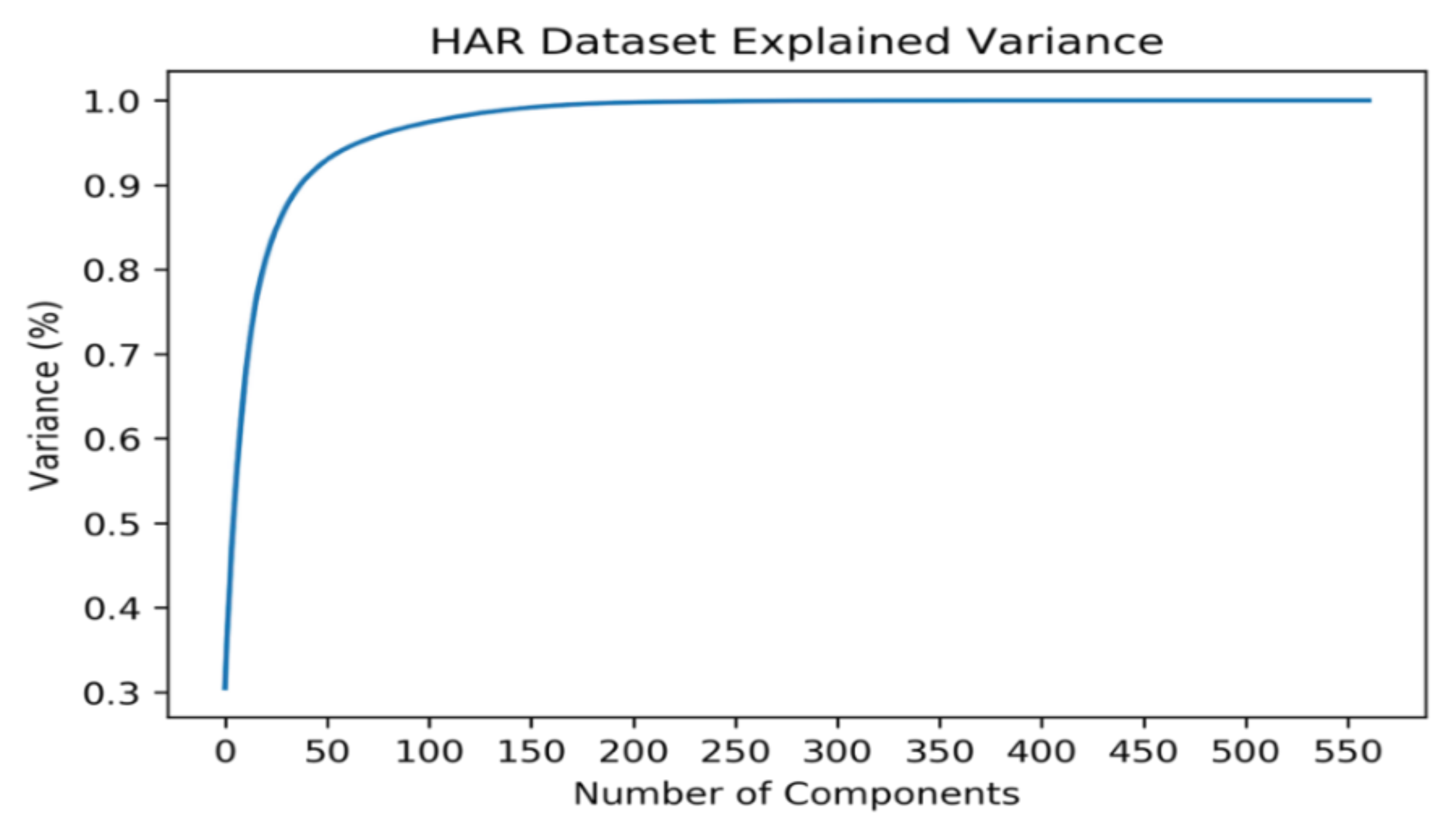
The plot in Figure 2 shows that by selecting 50 components, we can approximately preserve 92.82% of the total variance of the data. With this information in our hands, we can implement the PCA for the 50 best components. Here, we project 561-dimensional data to 50 principal components. Next, we get the transformed dataset. From the transformed dataset, we can determine the explained variance ratio. After that, we find the most important features from each principal component. The important features are the ones that influence more components and thus, have a large absolute value and score on the component. We have 50 important features and 2 of them are repeated. So, in total, we have 48 top features to model our data. We also have implemented the PCA for 100 components where we could preserve approximately 97.40% of the total variance of the data. In this situation, we have found the 100 most important features from each component but few of them are repeated. So, we have the top 92 features only to model our data. For 150 components, we have 99.16% data. From that, we have 138 most important features. Additionally, we could preserve 99.77% of the data for 200 principal components. Here, we have the 164 most important features to model our data.
4.4. Dataset Analysis
The focus of the proposed methodology is how to read the HAR dataset, understand it, and use the features. So, we have analyzed the dataset at the beginning. To do the analysis, we have used very well-known libraries such as Seaborn, Pandas, matplotlib, and NumPy.
4.5. Google Colab
Colaboratory is a Google research project, and it was created to help disseminate machine learning education and research. It is a Jupyter notebook environment, which can be used without any setup and runs entirely on the cloud [32].
Google offers free use of GPU and it is an attractive feature to the developers. The reasons for making it publicly available could be to make its software a standard in the field of academia for teaching machine learning and data science. They may also have a long-term plan to build a client base for Google Cloud APIs that are sold on a per-use basis [33].
By using Colab, programmers could write, edit, and execute code in python. Additionally, popular python libraries such as NumPy and Matplotlib could be used to analyze and visualize data [19]. It also allows us to integrate open-source libraries named PyTorch, TensorFlow, Keras, and OpenCV.
4.6. Keras
We have used Keras to implement CNN, and it is an open-source neural network library written in python. It has the capability to run on top of TensorFlow or Theano. It is designed for enabling fast experimentation with deep neural networks. The main model type of Keras is a sequence of layers called Sequential, and it is a linear stack of layers [34].
The construction of deep learning models in Keras is summarized below:
- Define our model: first, we create a Sequential model and add configured layers.
- Compile our model: after that, we specify loss function and optimizers and call the compile function on the model.
- Fit our model: in the next step, we call the fit function on the model and train the model on a sample of data.
- Make predictions: finally, we call functions named evaluate or predict and use the model to generate predictions on new data [34].
4.7. Convolutional Neural Network
A Convolutional Neural Network (CNN), a deep learning algorithm traditionally used for image classification, is now being utilized to solve ML problems in other domains. It is a multi-layer neural network designed to analyze visual inputs and perform different tasks. It can also be used for deep learning applications in healthcare [35]. More importantly, it works very well for the analysis of a time series of sensor data [36].
There are two main parts to a CNN:
- First is a convolution tool that splits the various features of the dataset for the analysis.
- Second is a fully connected layer that uses the output of the convolution layer to predict the best description for the activity.
A CNN is composed of several layers:
- Convolutional layer: in this layer, a feature map is created to predict the class probabilities for each feature by applying a filter that scans the features.
- Pooling layer: this layer scales down the amount of information the convolutional layer generated for each feature and maintains only the most essential information.
- Fully connected input layer: this layer “flattens” the outputs generated by previous layers and turns them into a single vector that could be used as an input for the next layer.
- Fully connected layer: this layer predicts an accurate label. It does that by applying weights over the input generated by the feature analysis.
- Fully connected output layer: it generates the final probabilities for determining a class for the activity [35].
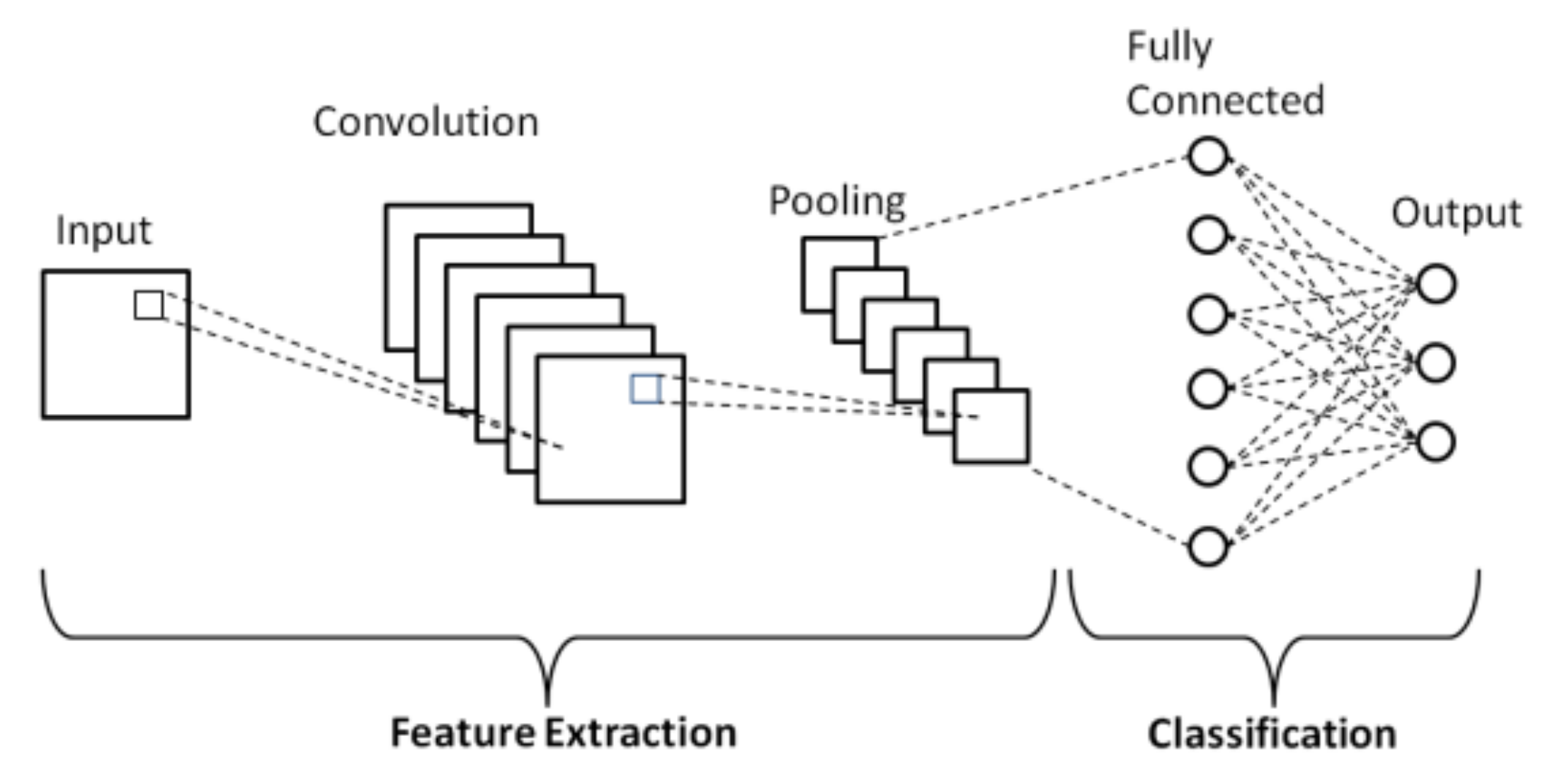
Figure 3 shows an example of a simple schematic representation of a basic CNN. This simple network consists of five different layers: an input layer, a convolution layer, a pooling layer, a fully connected layer, and an output layer. These layers are generally divided into two parts: feature extraction and classification [37].
4.8. Training Parameters
- Number of Epochs: The number of epochs is a hyperparameter that defines the number of times that the learning algorithm works through the entire training dataset. One epoch means that each sample in the training dataset will have an opportunity to update the internal model parameters. An epoch consists of one or more batches. The number of epochs allow the learning algorithm to run until the error from the model has been sufficiently minimized [38].
- Dense Layer: a “dense” layer that takes that vector and generates probabilities for six target labels, using a “Softmax” activation function [39].
- Optimizer: we use the “adam” optimize, which adjusts learning rate throughout training.
- Loss function: we use a “categorical_crossentropy” loss function, a common choice for classification. The lower the score, the better the model is performing.
- Metrics: we use the “accuracy” metric to get an accuracy score when the model runs on the testing set.
For our work, we have used two convolution layers, max pooling size of two, and two fully connected layers. We have used batch size of 64. We have kernel size of two. We could stop training our model earlier and it is supported by Keras. It is done via a callback called EarlyStopping. We have also used it and it has stopped training as soon as the validation loss reaches a minimum. This way, we have 25 as no. of epoch.
5. Experimental Data Analysis
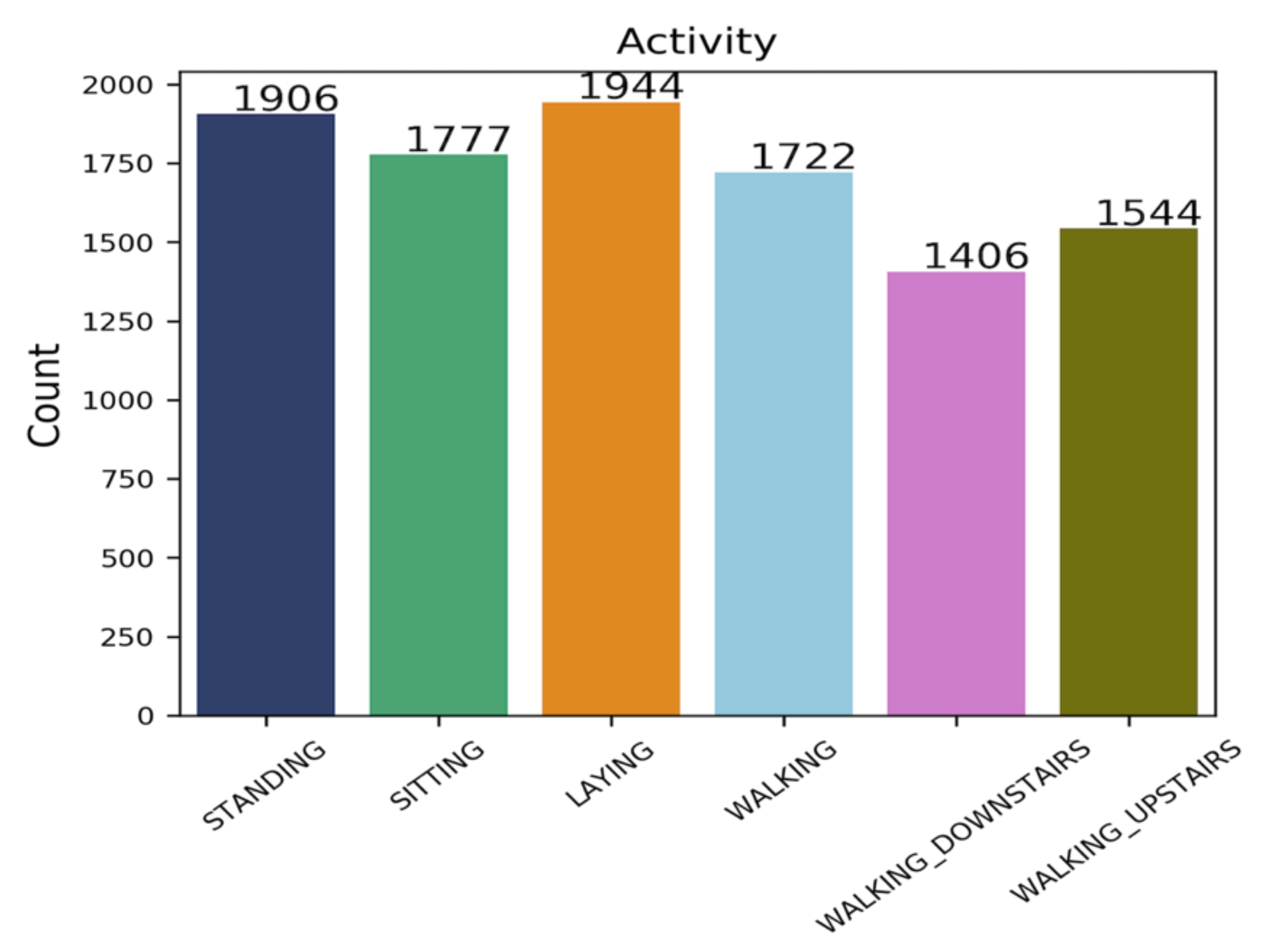
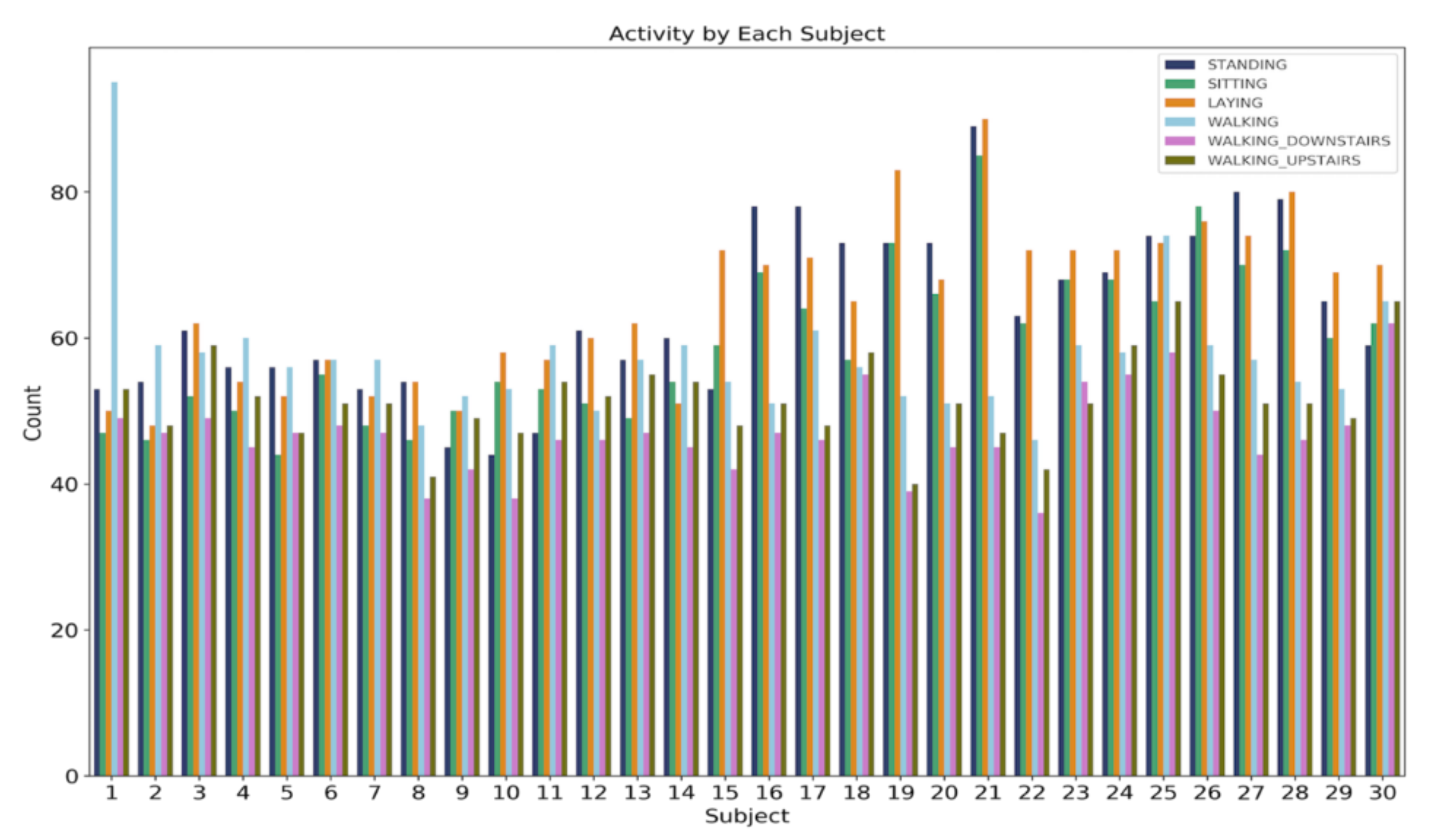
Here, we have presented and explained our data analysis. In order to analyze the dataset, we have used python. We have also implemented Pandas, Seaborn, matplotlib, NumPy etc. to do the analysis. At first, we have counted the different types of activities in the dataset. From Figure 4, we can see that the dataset is not imbalanced. STANDING is the Activity that is performed maximum no. of times, and WALKING_DOWNSTAIRS is the lowest performed Activity. Next, we can see from Figure 5 that there are six different types of Activity performed by different Subject.
6. Experiment
6.1. Experimental Setup
For our work, we have used Central Processing Unit (CPU) of Google Colab. The specifications of CPU runtime offered by Google Colab are Intel Xeon Processor with two cores @ 2.30 GHz and 13 GB RAM. The installed version of Python is 3.6.9 and Keras is 2.4.3.
6.2. Implementation of the Model
In this part, we have used CNN, which has been explained earlier. Later, we have implemented them to compare the overall accuracy and loss. Additionally, we have calculated the confusion matrix to find out how well our model performs.
The following parameters are used for the confusion matrix:
- True Positive (TP): how often the model correctly predicts the right activity.
- True Negative (TN): indicates how the model correctly predicts a person not doing that particular activity.
- False Positive (FP): how often the model predicts a person doing the particular activity when he/she is not actually doing that activity.
- False Negative (FN): indicates how often the model predicts a person not doing the particular activity when he/she is in fact doing that activity.
Moreover, we have also collected the results for the parameters below:
- Accuracy: accuracy is simply a proportion of observations correctly predicted to the total observations [40].
- Loss in CNN: loss is the quantitative measure of deviation or difference between the predicted output and the actual output. It measures the mistakes made by the network in predicting the output.
Accuracy = (TP + TN)/(TP + FP + FN + TN),
7. Implementation Details and Results
We have done the experiment with all the features of the dataset to do the CNN model. Additionally, we have run the experiment with a hybrid approach where we use the most important features of the dataset to do the modeling of CNN. In the experiment, for the evaluation of our proposed methodology, datasets are split into two different ratios such as 70–10–20% and 80–10–10% for training, validation, and testing, respectively.
For our work, we have used Keras deep learning library for implementing the CNN model. The model is defined as a Sequential Keras model. We can extract the input and output dimensions from the given training dataset and fit them into our model. The output for the model will be a six-element vector that contains the probability of a given window belonging to each of the six activities. We have fit the model for 25 epochs and used a batch size of 64 samples. The 64 windows of data will be exposed to the model before the weights of the model are updated. Once the model is fit, it is evaluated on the test dataset. After that, the accuracy of the fit model on the test dataset is returned along with the validation loss. Additionally, we have the confusion matrix.
At the beginning, we have executed the experiment without extracting any features in the preprocessing step for 70–10–20% split ratio. We have executed the trained model with epoch size of 25. First, we have the accuracy and loss for the trained model. After that, we have the confusion matrix where the diagonal values refer to the true positive values for the six activities (please see Appendix A).
Next, we will be discussing each layer below for our work:
- Input Data: First, we have 7209 samples and 561 features of the dataset as an input to the CNN model. We have got those from the training part of the dataset.
- First 1D CNN Layer: The first layer defines a filter of kernel size 2. If we define one filter in the first layer, then it would allow the neural network to learn only one feature. This might not be enough; therefore, we have defined 128 filters. This allows us to train 128 different features on the first layer of the network. We get (560 × 128) neuron matrix as an output of the first neural network layer. The individual columns of the output matrix hold the weights of one single filter. With the defined kernel size and length of the input matrix, each filter will be containing 560 weights.
- Second 1D CNN Layer: The result we get from the first CNN will get fed into the second CNN layer. We will define 64 different filters to be trained on this level. The logic of the first layer applies here as well, so the output matrix will have a size of (559 × 64).
- Max Pooling Layer: Because we need to reduce the complexity of the output and prevent overfitting of the data, a pooling layer is often used after a CNN layer. In our work, we have chosen two as a pooling size. This means that the size of the output matrix is only half of the input matrix. The size of the matrix is (279 × 64).
- Flatten Layer: There is a ‘flatten’ layer in between the convolutional layer and the fully connected layer. A two-dimensional matrix (279 × 64) of features is transformed into a vector (17,856) by flattening. After that, the vector could be fed into a fully connected neural network classifier.
- Dense Layer: In this layer, the results of the convolutional layers are generally fed through one or more neural layers to generate a prediction.
- Fully Connected Layer with “Softmax” Activation: The final layer reduces the vector of height 64 to a vector of six since we have six classes that we want to predict. This reduction process is achieved by another matrix multiplication. We have used “Softmax” as the activation function and it enforces all six outputs of the neural network to sum up to one. Therefore, the output value will be representing the probability for each of the six classes [41].
Then, we have the results for our hybrid approach where we have used PCA as a preprocessing step to extract the most important features and then fed those features to train the CNN models. By using principal components 200, 150, 100, and 50, we have got 164, 138, 92, and 48 important features.
Here, we discuss the CNN model with 200 principal components, where we have 164 important features. We have executed the trained model with epoch size of 25. First, we have the accuracy and loss for the trained model. After that, we have the confusion matrix.
The details of the layers are discussed below for this case:
- Input Data: First, we have 7209 samples and 164 features of the dataset as an input to the CNN model. We have got those from the training part of the dataset.
- First 1D CNN Layer: The first layer defines a filter of kernel size two. Here, we have defined 128 filters. This allows us to train 128 different features on the first layer of the network. We get (199 × 128) neuron matrix as an output of the first neural network layer. The individual columns of the output matrix hold the weights of one single filter. With the defined kernel size and length of the input matrix, each filter will contain 199 weights.
- Second 1D CNN layer: The result we get from the first CNN will be fed into the second CNN layer. We will define 64 different filters to be trained on this level. The logic of the first layer applies here as well, so the output matrix will have a size of (198 × 64).
- Max pooling layer: In this case, we have chosen two as a pooling size. This means that the size of the output matrix of this layer is only half of the input matrix. The size of the matrix is (99 × 64).
- Flatten Layer: A two-dimensional matrix (99 × 64) of features is transformed into a vector (6336) by flattening. After that, the vector could be fed into a fully connected neural network classifier.
- Dense Layer: In this layer, the results of the convolutional layers are generally fed through one or more neural layers to generate a prediction.
- Fully Connected Layer with “Softmax” Activation: The final layer reduces the vector of height 64 to a vector of 6 since we have 6 classes that we want to predict. This reduction process is achieved by another matrix multiplication. We have used “Softmax” as the activation function and it enforces all six outputs of the neural network to sum up to one. Therefore, the output value will represent the probability for each of the six classes [41].
For the other cases, we have done the experiments where we have the corresponding input data for the other principal components. In general, the procedure remains the same. For the other split ratio, we have the same kind of set up for the experiments.
7.1. 70%–Training, 10%–Validation, 20%–Testing
7.1.1. All Features
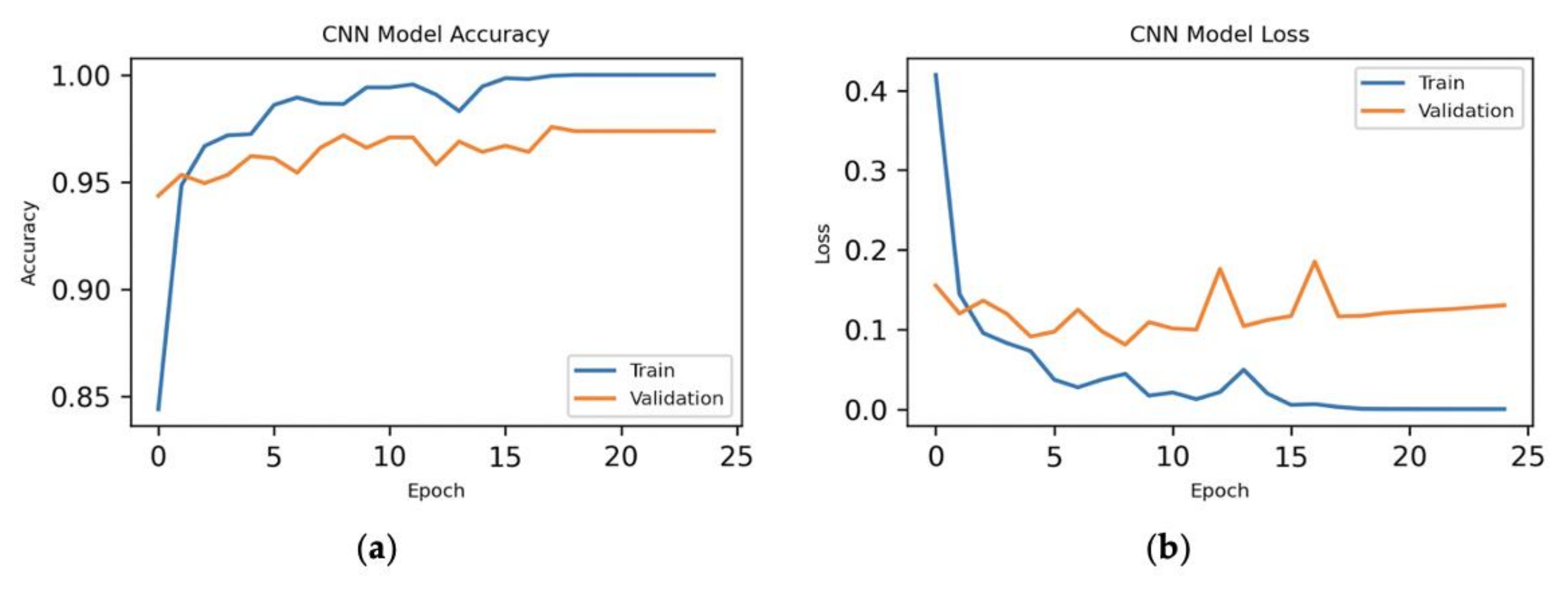
Here, we have executed the experiment with all the features of the dataset to do the CNN model and could see the experimental results in Figure 6. We can see from the figure that the loss is minimum from epoch 18 to 25 for our model.
7.1.2. Hybrid Approach
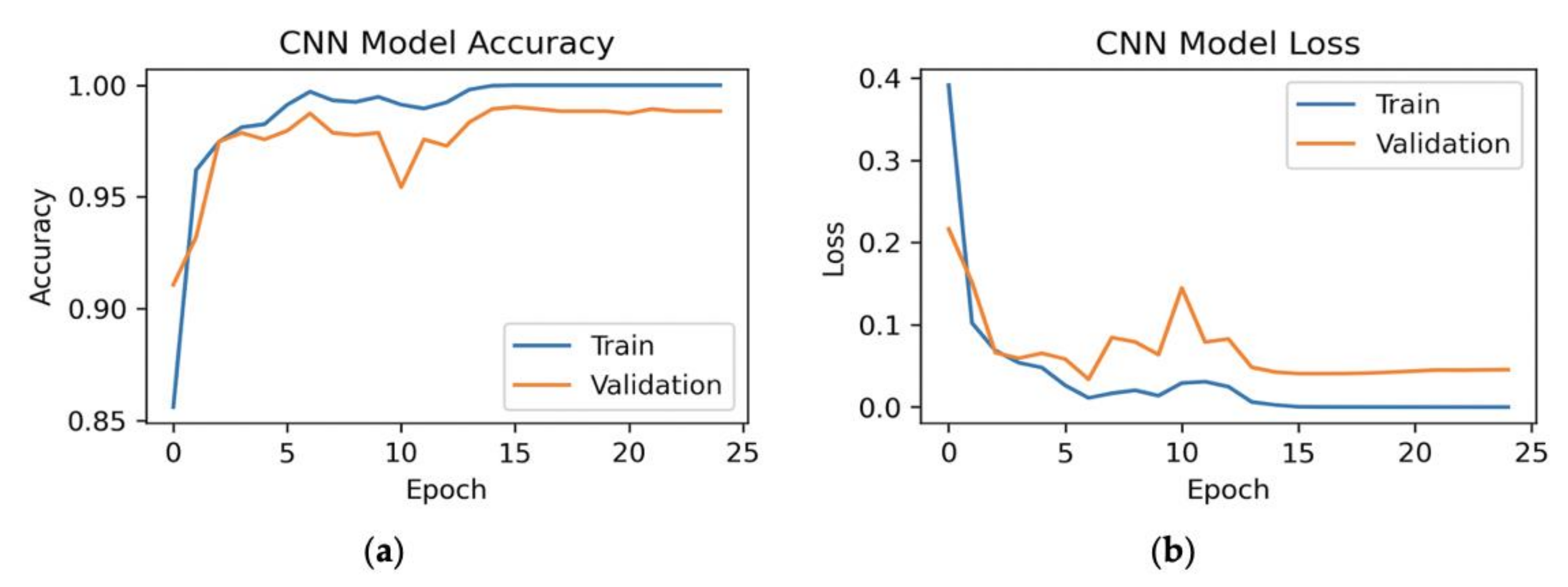
Here, we have executed the experiment for CNN with 50 principal components, where we have the 48 most important features of the dataset for the model and shown the results in Figure 7.
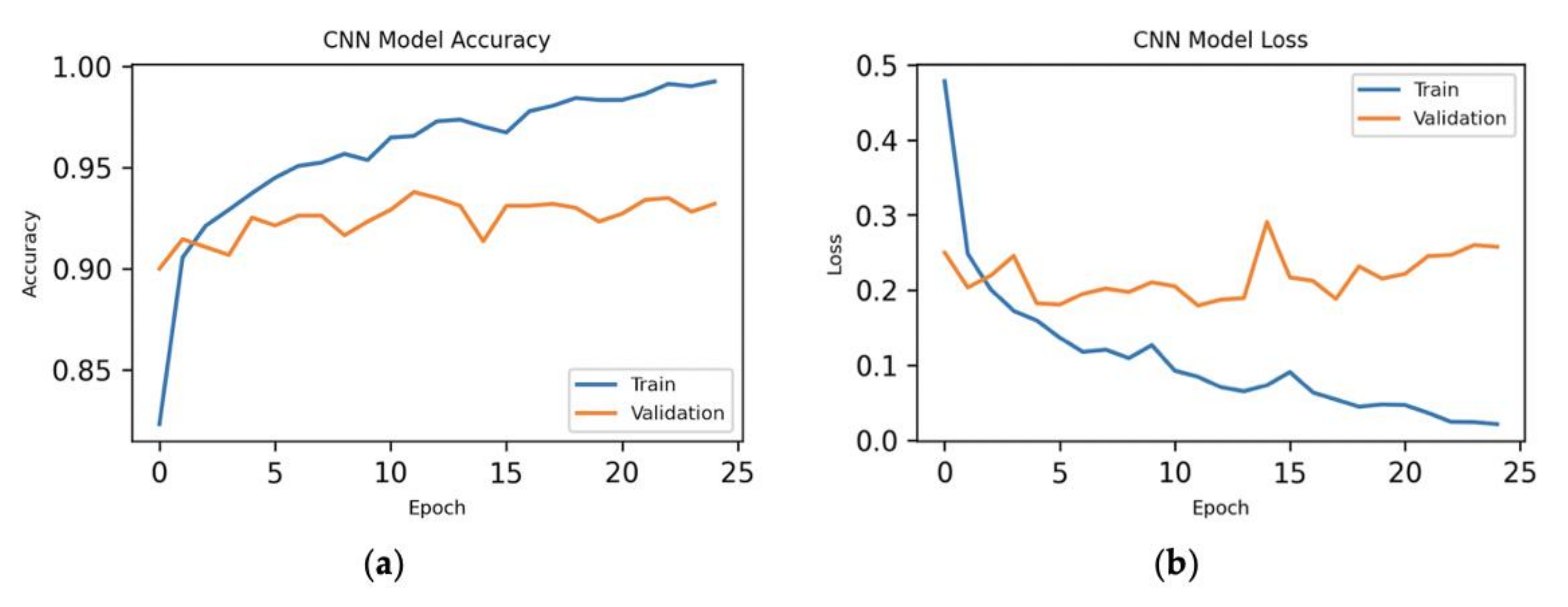
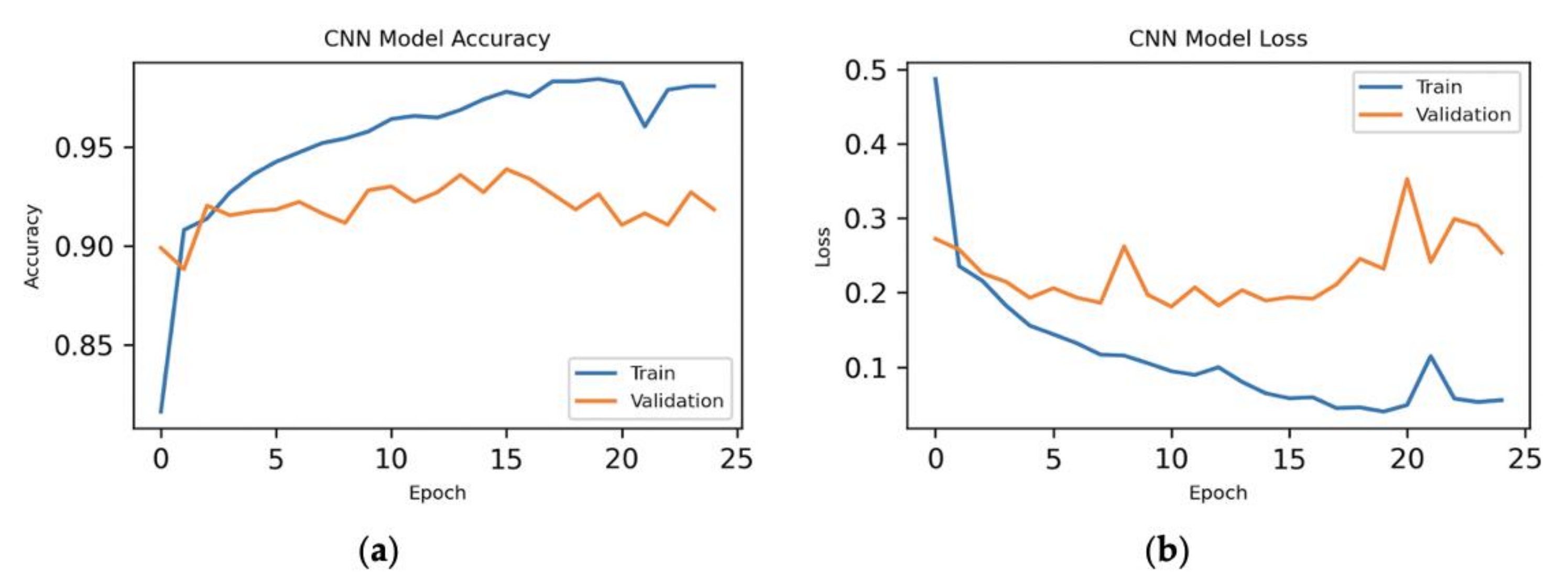
Next, we have executed the experiment for CNN with 100 principal components, where we have the 92 most important features of the dataset for the model. We could see the results in Figure 8.
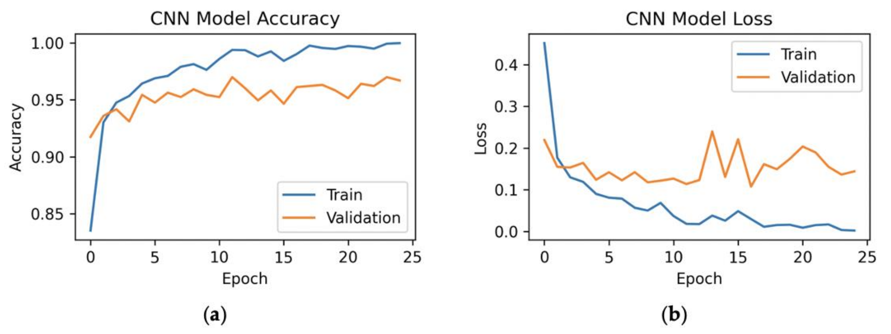
After that, we have done the experiment for CNN with 150 principal components, where we have obtained the 138 most important features of the dataset for the model and results are shown in Figure 9.
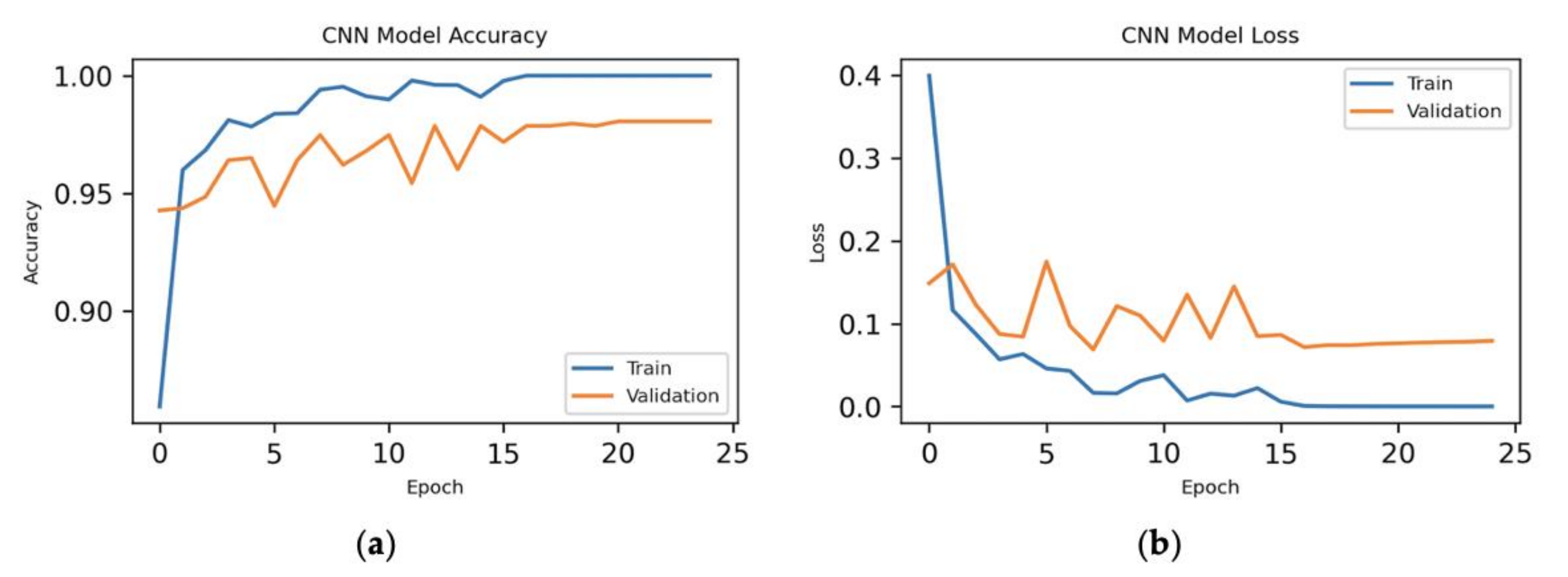
Next, we have done the experiment for CNN with 200 principal components, where we have obtained 164 most important features of the dataset for the model. We could see the results in Figure 10. Here, the loss is minimum from epoch 17 to 25 for our model.
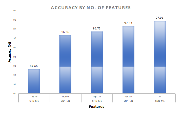
Figure 11 shows the effect of number of features on accuracy for the current split ratio.
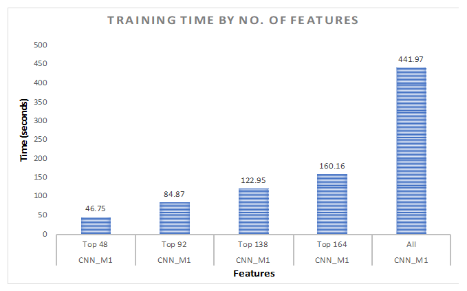
Figure 12 shows the time taken to train the model by using the top features as well as all the features.
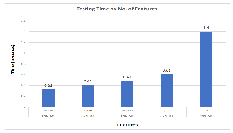
We can then see the effect of number of features on testing time in Figure 13.
We have run the testing part 1000 times. For all features, the average computation time was 1.33 s. On the other hand, it took 0.23 s with 48 features. This way, we could save around 83% testing time. With 92 features, we are able to save 74.44% time. The time taken to test with 138 features is 0.46 s. In this case, we could save around 65.5% testing time. Finally, with 164 features the testing time is 0.55 s. For this case, we are able to save around 59.65% testing time. It could be said that the average computation time is improved significantly as we are reducing the number of features.
7.2. 80%–Training, 10%–Validation, 10%–Testing
7.2.1. All Features
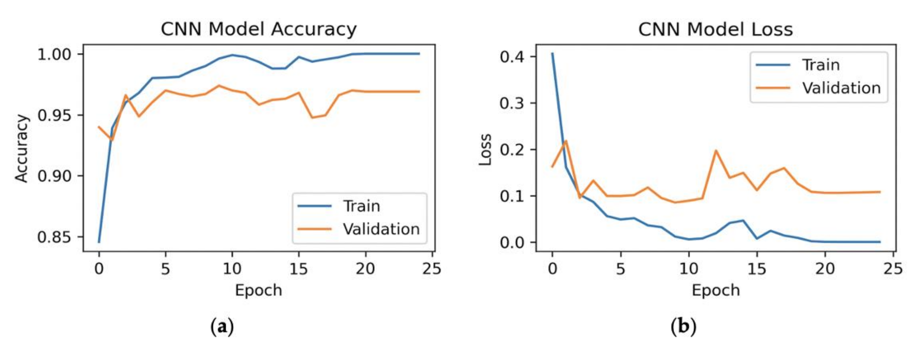
Here, we have executed the experiment with all the features of the dataset to do the CNN model. The results are shown in Figure 14.
7.2.2. Hybrid Approach
Here, we have done the experiment for CNN with 50 principal components, where we have obtained the 48 most important features of the dataset for the model. The experimental results are shown in Figure 15.
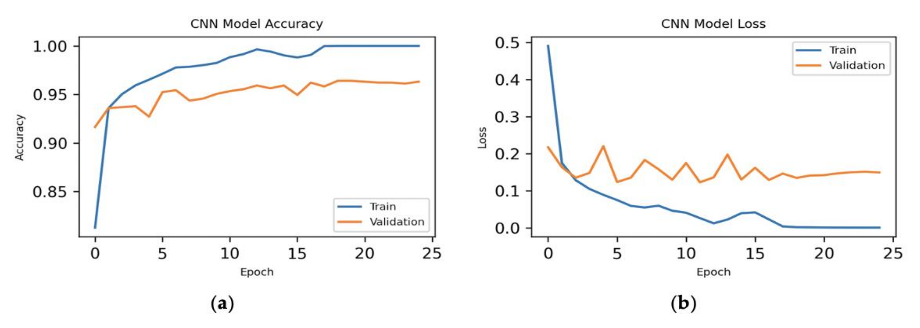
Next, we have done the experiment for CNN with 100 principal components, where we have obtained the 92 most important features of the dataset for the model and shown the results in Figure 16.
After that, we have done the experiment for CNN with 150 principal components, where we have obtained the 138 most important features of the dataset for the model. The experimental results could be seen in Figure 17.
Finally, we have done the experiment for CNN with 200 principal components, where we have obtained the 164 most important features of the dataset for the model. The experimental results are shown in Figure 18.
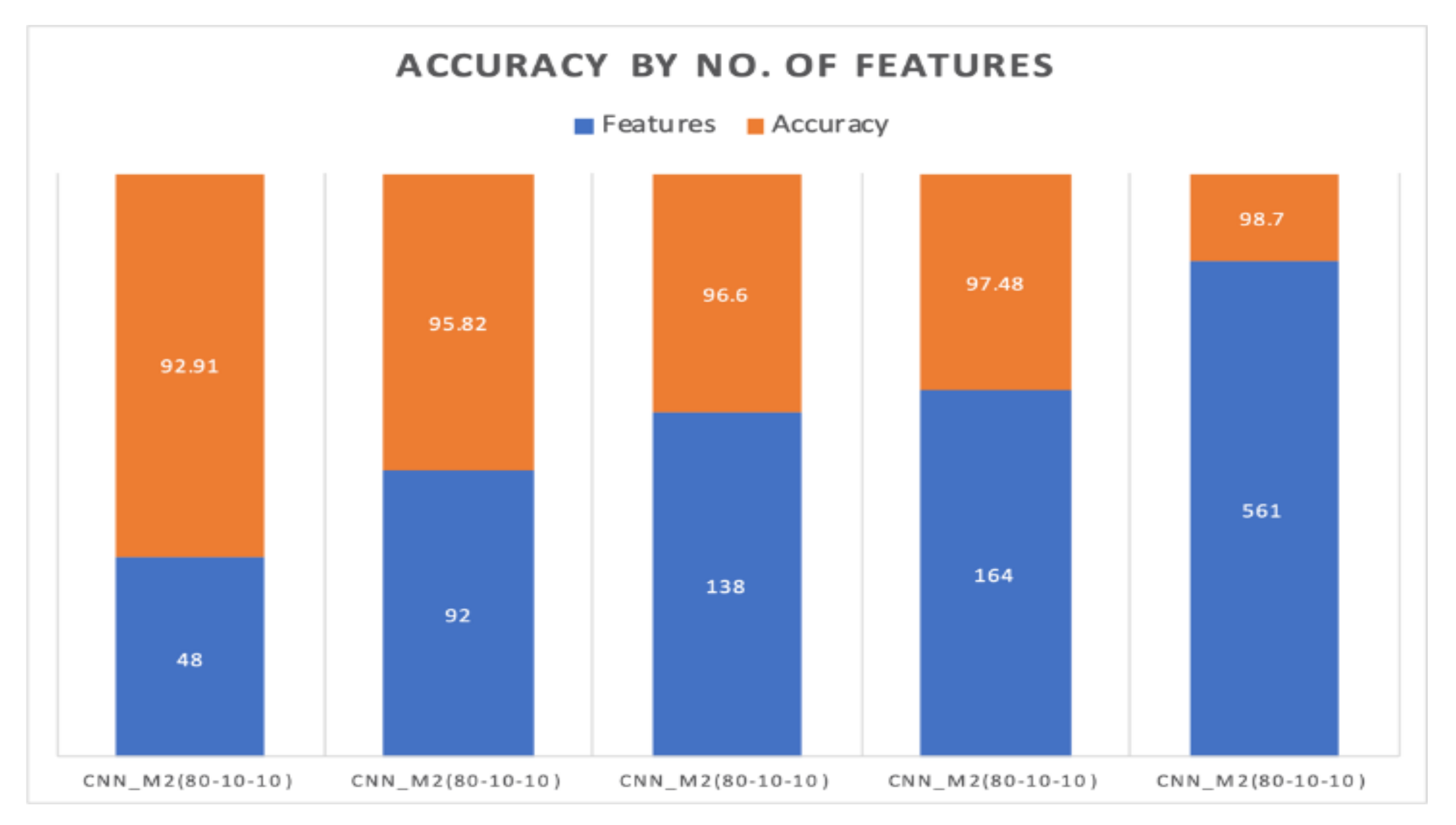
Figure 19 shows the effect of number of features on accuracy for the current split ratio.
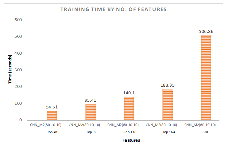
Here, Figure 20 shows the time taken to train the model by using the top features as well as all the features.
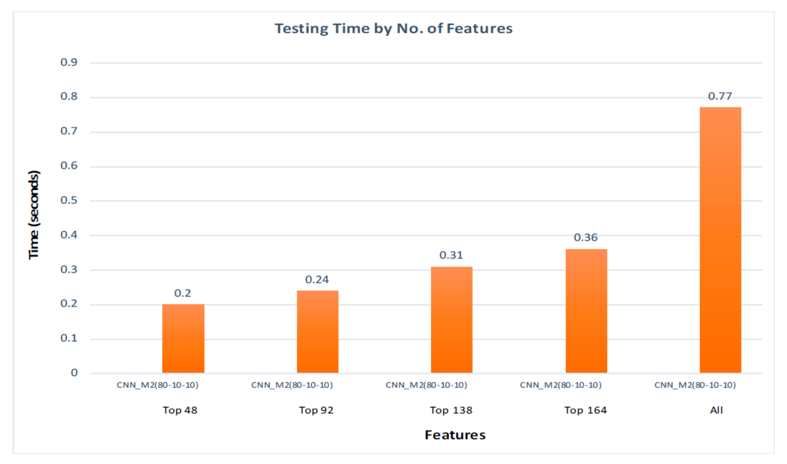
We can then see the effect of number of features on testing time in Figure 21.
Furthermore, for 80–10–10% split ratio, we have executed the testing part 1000 times. For all the features, the average computation time was 0.68 s. On the other hand, it took 0.15 s with 48 features. This way, we could save around 78% testing time. With 92 features, we are able to save 69.6% time. The time taken to test with 138 features is 0.26 s. In this case, we could save around 61.76% testing time. Finally, with 164 features the testing time is 0.30 s. For this case, we are able to save around 56% testing time. Here, we have improved the average calculation time by using the top features of the dataset.
We have set the performance of CNN (70% training–10% validation–20% testing) with 48 features as a benchmark for our work. For 70–10–20% ratio, we have achieved maximum accuracy of 97.91% with all the features. As we are increasing the number of features from 48 to 92, we have achieved better accuracy (96.36%). It could be observed from Figure 11 that there is a slight increase in the accuracy for 138 features compared to the accuracy of 92 features. With 164 features, we have achieved an accuracy of 97.33%. For the training time with the same ratio, it took 441.97 s to train the model with all the features. We have then trained the model with 48 features of the dataset and the training time was improved. After that, we have trained the model with 92, 138, and 164 features, respectively. We can see that it is taking more time to train the model as we increase the number of features. On the other hand, we have improved the training time a lot by only using the top features. Additionally, we have improved the testing time compared to the time taken for all the features.
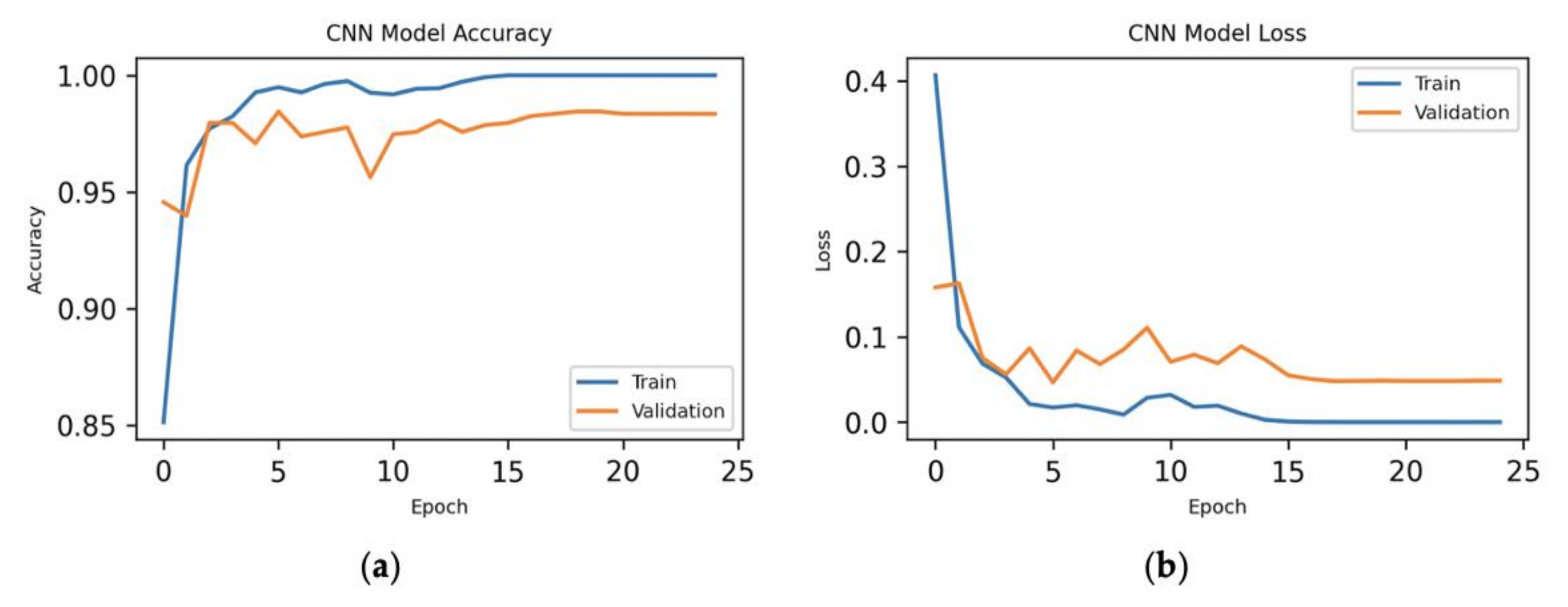
For the ratio of 80–10–10%, we have achieved maximum accuracy of 98.70% with all the features of the dataset. With 164 features, we have achieved the second maximum accuracy with the same ratio. In this case, the training time and testing time have also improved significantly because of using the top features of the dataset.
We have also reduced the training time from 506.86 s to 84.87 s by using 92 features of the dataset. This way, we could save 83.26% time to train our model.
It could be observed that we have improved not only the training time but also the testing time from 0.77 s to 0.41 s.
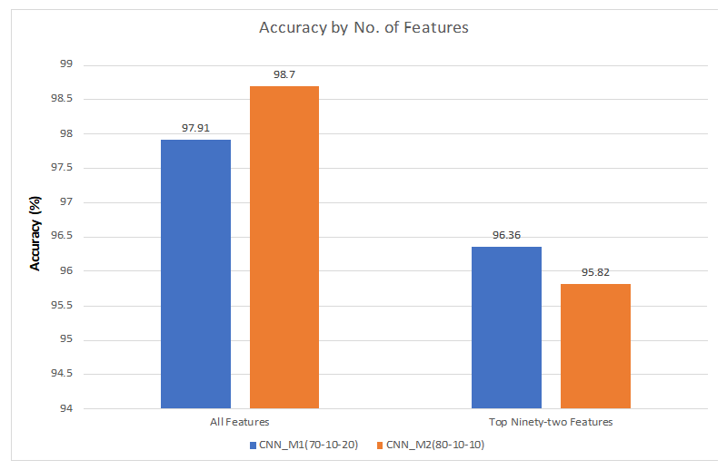
Figure 22 shows the accuracy by number of features for different split ratio. We could see that we have got better accuracy with all the features for 80–10–10% split ratio compared to the accuracy of the other split ratio. On the other hand, we have obtained higher accuracy with 92 features for 70–10–20% ratio than the other split ratio.
If we compare our accuracy with Sikder et al. [22], we have achieved better accuracy using hybrid approach with 92 features of the dataset.
8. Conclusions and Future Work
In this paper, we have proposed a method that utilizes a cloud-based platform for HAR. The results show that by using our method, we have achieved 96.36% accuracy for the top 92 features. By reducing the number of features to 92, we have sped up the training and testing time of ML algorithms. It can be noted that we have achieved better results as compared to the results obtained by Sikder et al. [22] with the same dataset but using only 92 features for the model.
To conclude, the importance of dimensionality reduction for HAR has been discussed in this work. The experimental results have shown that reduction of the data allows us to achieve good accuracy compared to other researchers. Furthermore, training time and testing time of the model have been improved significantly than the time required for the original dimension of the input space.
We can extend our work in the future by adding more layers to the CNN model. We can also extend our work by using other deep learning algorithms. There are different types of algorithms used nowadays: Multilayer Perceptron Neural Network (MLPNN), Recurrent Neural Network (RNN), Long Short-Term Memory (LSTM), and Generative Adversarial Network (GAN). Among all the algorithms, we can use LSTM. The advantage of using LSTM is that the input values fed to the network not only go through several LSTM layers but also propagate through time within one LSTM cell. Hence, parameters are well distributed within multiple layers. This results in a thorough process of inputs in each time step [42].
Because it is common to use CNN nowadays for time series data, the proposed method should work for HAR other than the data collected by only using accelerometer and gyroscope of a smartphone. We could make sure of that by using other datasets such as smart home, where we have different types of sensors generate data continuously. Furthermore, if we feed our model with more data then it will be stronger and achieve better performance. On the other hand, if we have a small dataset then it might perform poorly because we will be feeding CNN with less data. It would run into an overfitting problem. But if we have a huge dataset with a size of a gigabyte, then the model might take a lot of time to train the data. In this situation, we might need to use GPUs to improve it.
Author Contributions
Conceptualization, S.R.; methodology, S.R.; experiment, S.R.; resources, S.R.; dataset collection, S.R.; dataset analysis, K.A.; writing—original draft preparation, S.R. and K.A.; writing—review and editing, D.P.A. and S.R.; supervision, D.P.A.; project administration, D.P.A. All authors have read and agreed to the published version of the manuscript.
Funding
This research received no external funding.
Conflicts of Interest
The authors declare no conflict of interest.
Appendix A
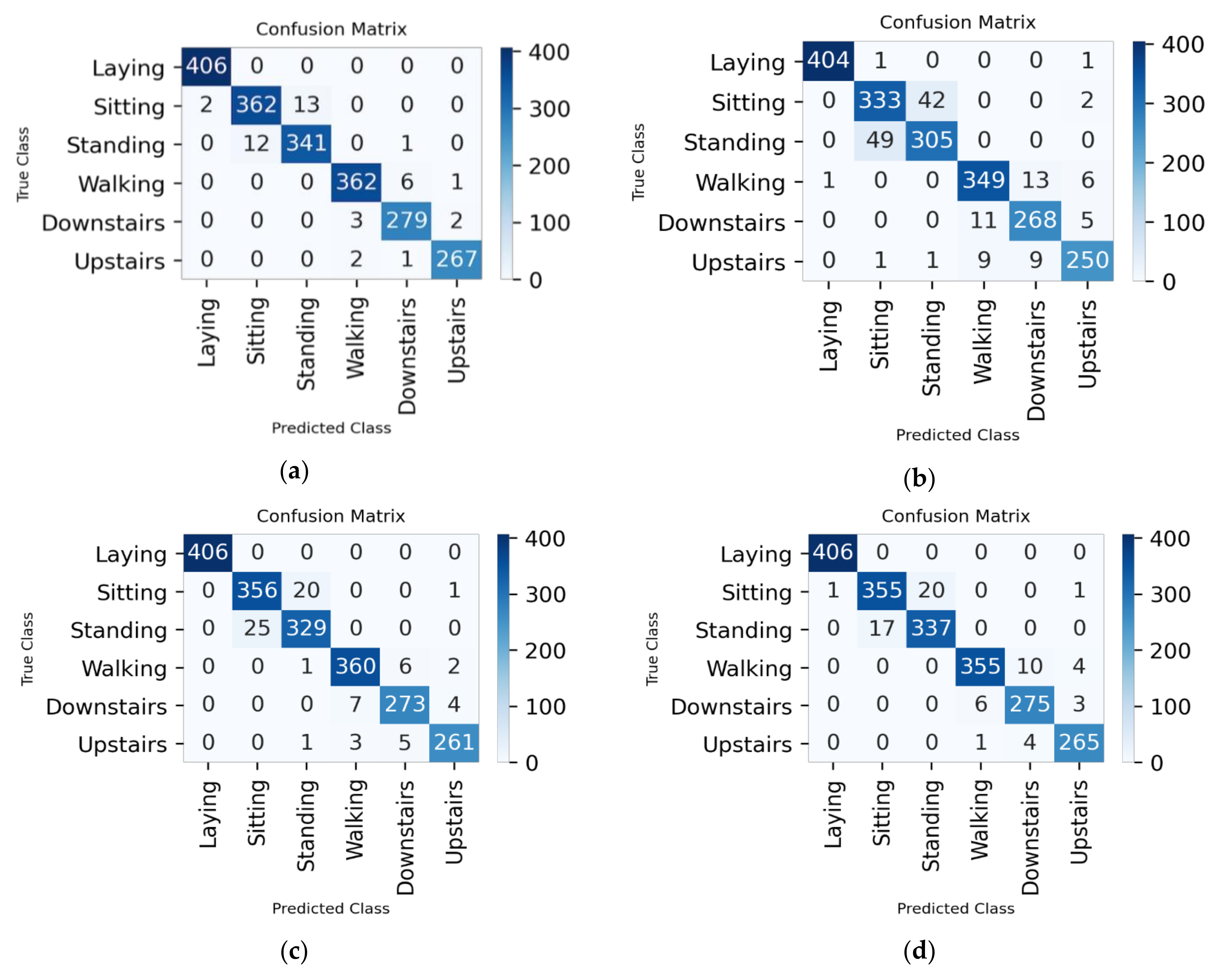
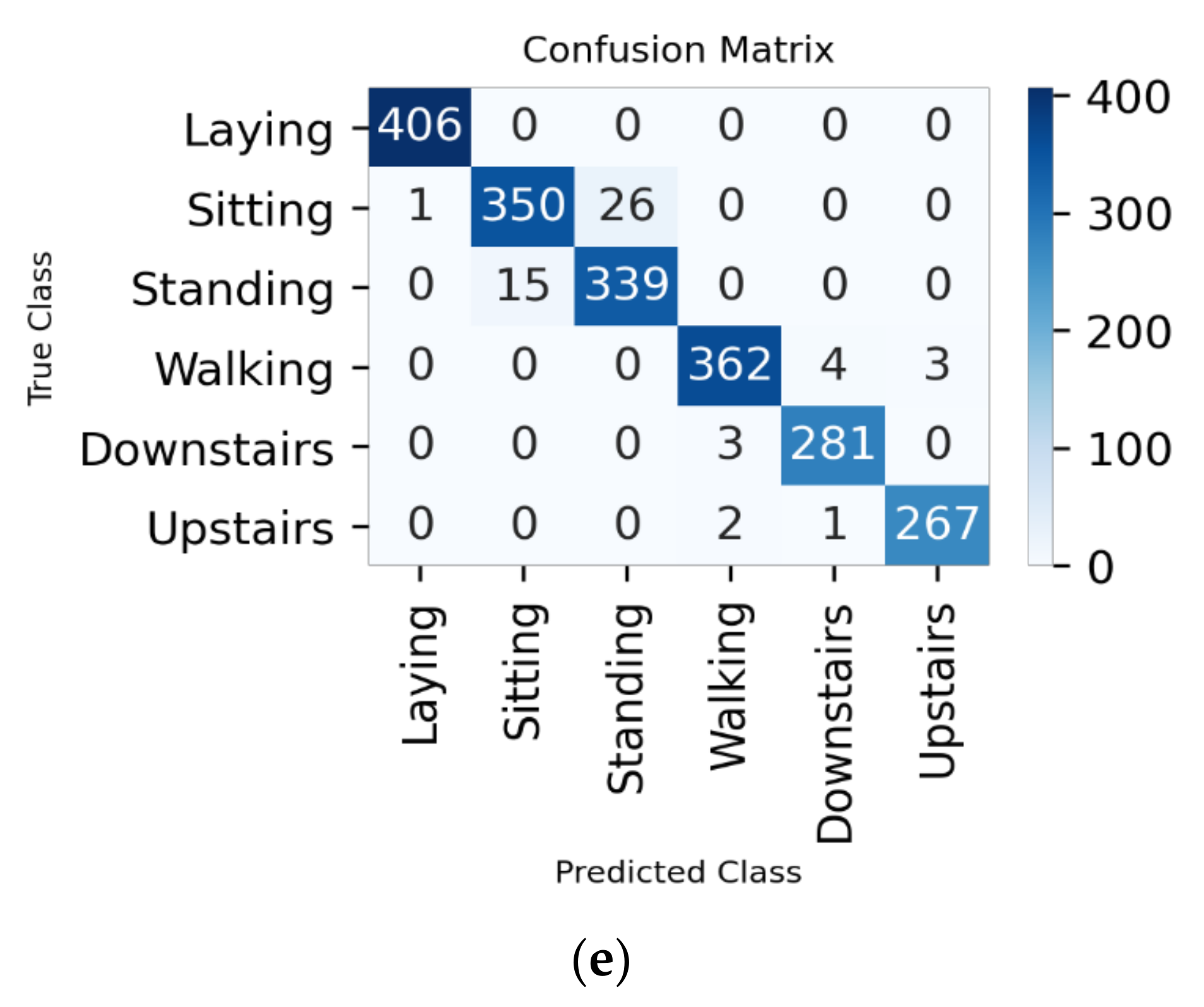
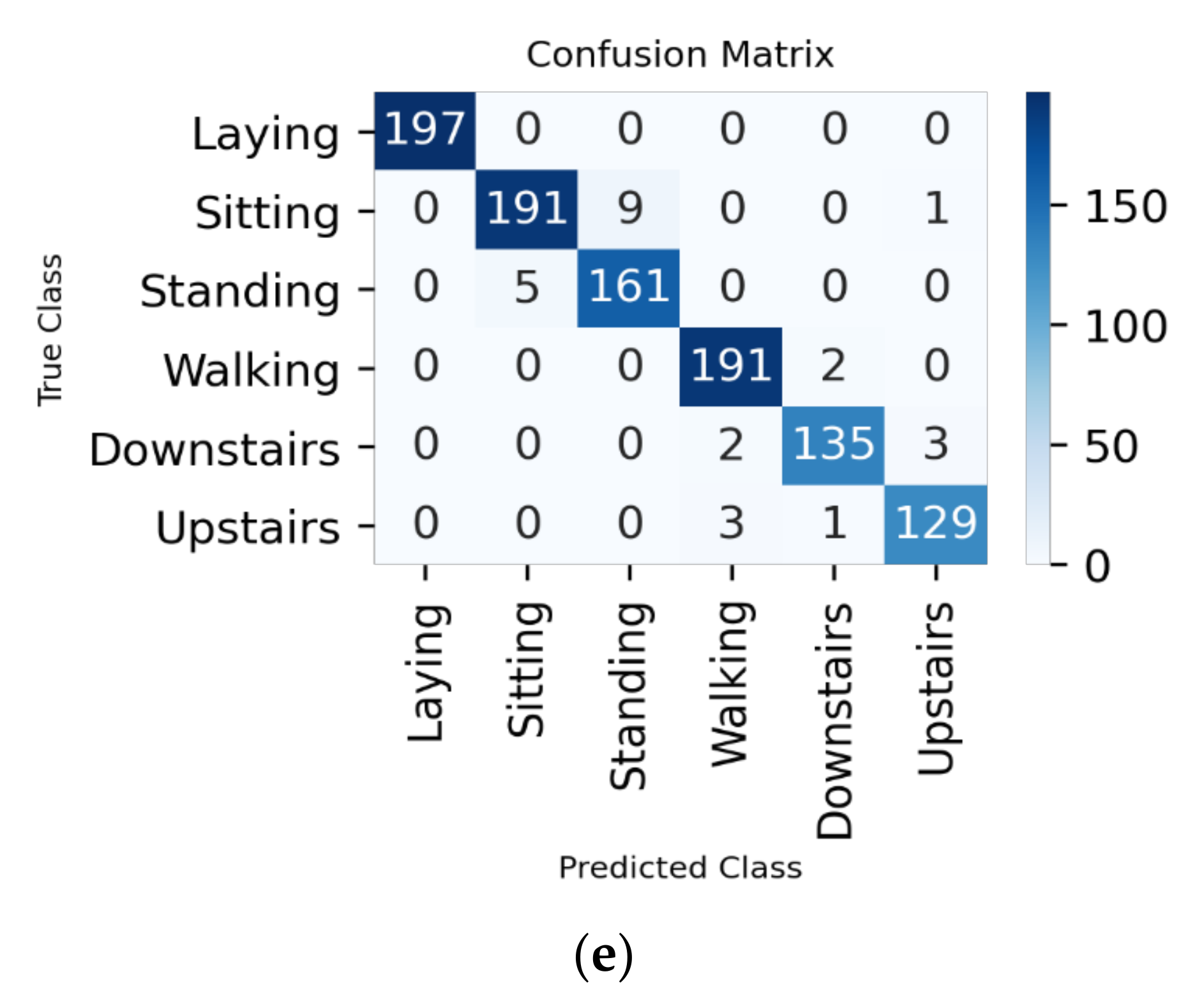
Figure A1.
Confusion matrix for 70–10–20% split ratio: (a) all the features; (b) 48 features; (c) 92 features; (d) 138 features; and (e) 164 features.
Figure A1.
Confusion matrix for 70–10–20% split ratio: (a) all the features; (b) 48 features; (c) 92 features; (d) 138 features; and (e) 164 features.


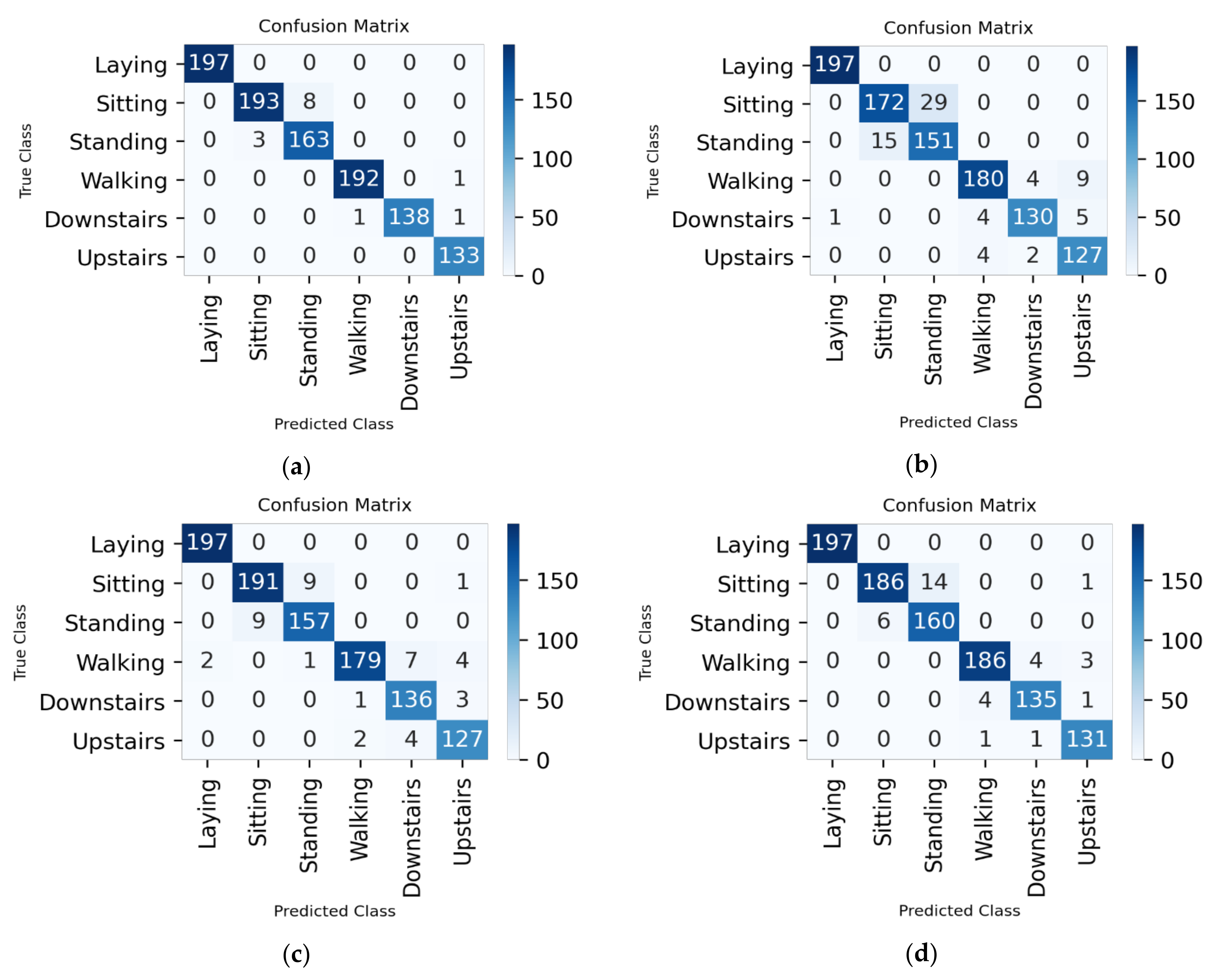
Figure A2.
Confusion matrix for 80–10–10% split ratio: (a) all the features; (b) 48 features; (c) 92 features; (d) 138 features; and (e) 164 features.
Figure A2.
Confusion matrix for 80–10–10% split ratio: (a) all the features; (b) 48 features; (c) 92 features; (d) 138 features; and (e) 164 features.


References
- Brastein, O.M.; Olsson, R.; Skeie, N.O.; Lindblad, T. Human Activity Recognition by machine learning methods. In Proceedings of the Norsk IKT-Konferanse for Forskning Og Utdanning, Oslo, Norway, 27–29 November 2017. [Google Scholar]
- Roy, S.; Edan, Y. Investigating joint-action in short-cycle repetitive handover tasks: The role of giver versus receiver and its implications for human-robot collaborative system design. Int. J. Soc. Robot. 2018, 12, 973–988. [Google Scholar] [CrossRef]
- Wang, L.; Gao, R.; Váncza, J.; Krüger, J.; Wang, X.V.; Makris, S.; Chryssolouris, G. Symbiotic human-robot collaborative assembly. CIRP Ann. 2019, 68, 701–726. [Google Scholar] [CrossRef] [Green Version]
- Chen, Y.H.; Tsai, M.J.; Fu, L.C.; Chen, C.H.; Wu, C.L.; Zeng, Y.C. Monitoring elder’s living activity using ambient and body sensor network in smart home. In Proceedings of the 2015 IEEE International Conference on Systems, Man, and Cybernetics, Kowloon, Hong Kong, China, 9–12 October 2015; pp. 2962–2967. [Google Scholar]
- Spörri, J.; Kröll, J.; Fasel, B.; Aminian, K.; Müller, E. The Use of Body Worn Sensors for Detecting the Vibrations Acting on the Lower Back in Alpine Ski Racing. Front. Physiol. 2017, 8, 522. [Google Scholar] [CrossRef] [PubMed]
- Lee, W.; Cho, S.; Chu, P.; Vu, H.; Helal, S.; Song, W.; Jeong, Y.S.; Cho, K. Automatic agent generation for IoT-based smart house simulator. Neurocomputing 2016, 209, 14–24. [Google Scholar] [CrossRef]
- Ullah, M.; Ullah, H.; Khan, S.D.; Cheikh, F.A. Stacked Lstm Network for Human Activity Recognition Using Smartphone Data. In Proceedings of the 2019 8th European Workshop on Visual Information Processing (EUVIP), Roma, Italy, 28–31 October 2019; pp. 175–180. [Google Scholar]
- Ogbuabor, G.; La, R. Human activity recognition for healthcare using smartphones. In Proceedings of the 2018 10th International Conference on Machine Learning and Computing (ICMLC), Macau, China, 26–28 February 2018; pp. 41–46. [Google Scholar]
- Gjoreski, M.; Gjoreski, H.; Luštrek, M.; Gams, M. How accurately can your wrist device recognize daily activities and detect falls? Sensors 2016, 16, 800. [Google Scholar] [CrossRef] [PubMed]
- Lara, O.D.; Labrador, M.A. A survey on human activity recognition using wearable sensors. IEEE Commun. Surv. Tutor. 2012, 15, 1192–1209. [Google Scholar] [CrossRef]
- Avci, A.; Bosch, S.; Marin-Perianu, M.; Marin-Perianu, R.; Havinga, P. Activity recognition using inertial sensing for healthcare, wellbeing and sports applications: A survey. In Proceedings of the 23rd International Conference on Architecture of Computing Systems, Hannover, Germany, 22–25 February 2010; pp. 1–10. [Google Scholar]
- Alford, L. What men should know about the impact of physical activity on their health. Int. J. Clin. Pract. 2010, 64, 1731. [Google Scholar] [CrossRef] [PubMed] [Green Version]
- Kwak, T.; Song, A.; Kim, Y. The Impact of the PCA Dimensionality Reduction for CNN based Hyperspectral Image Classification. Korean J. Remote Sens. 2019, 35, 959–971. [Google Scholar]
- HAR Dataset. Available online: https://www.kaggle.com/uciml/human-activity-recognition-with-smartphones (accessed on 12 March 2020).
- Anguita, D.; Ghio, A.; Oneto, L.; Parra, X.; Reyes-Ortiz, J.L. A Public Domain Dataset for Human Activity Recognition Using Smartphones. In Proceedings of the 21st European Symposium on Artificial Neural Networks, Computational Intelligence and Machine Learning (ESANN), Bruges, Belgium, 24–26 April 2013. [Google Scholar]
- Anguita, D.; Ghio, A.; Oneto, L.; Parra, X.; Reyes-Ortiz, J.L. Human activity recognition on smartphones using a multiclass hardware-friendly support vector machine. In 4th International Workshop on Ambient Assisted Living; Springer: Vitoria-Gasteiz, Spain, 2012; pp. 216–223. [Google Scholar]
- Anguita, D.; Ghio, A.; Oneto, L.; Parra, X.; Reyes-Ortiz, J.L. Energy Efficient Smartphone-Based Activity Recognition using Fixed-Point Arithmetic. J. UCS 2013, 19, 1295–1314. [Google Scholar]
- Reyes-Ortiz, J.L.; Ghio, A.; Parra, X.; Anguita, D.; Cabestany, J.; Catala, A. Human Activity and Motion Disorder Recognition: Towards smarter Interactive Cognitive Environments. In Proceedings of the 21st European Symposium on Artificial Neural Networks, Computational Intelligence and Machine Learning (ESANN), Bruges, Belgium, 24–26 April 2013. [Google Scholar]
- Google. What is Colaboratory. Available online: https://colab.research.google.com/notebooks/intro.ipynb (accessed on 15 March 2020).
- Ray, S.; AlGhamdi, A.; Alshouiliy, K.; Agrawal, D.P. Selecting Features for Breast Cancer Analysis and Prediction. In Proceedings of the 6th International Conference on Advances in Computing and Communication Engineering (ICACCE), Las Vegas, NV, USA, 22–24 June 2020; pp. 1–6. [Google Scholar]
- Ahmed, N.; Rafiq, J.I.; Islam, M.R. Enhanced human activity recognition based on smartphone sensor data using hybrid feature selection model. Sensors 2020, 20, 317. [Google Scholar] [CrossRef] [PubMed] [Green Version]
- Sikder, N.; Chowdhury, M.S.; Arif, A.S.; Nahid, A.A. Human Activity Recognition Using Multichannel Convolutional Neural Network. In Proceedings of the 2019 5th International Conference on Advances in Electrical Engineering (ICAEE), Dhaka, Bangladesh, 26–28 September 2019; pp. 560–565. [Google Scholar]
- Gaur, S.; Gupta, G.P. Framework for Monitoring and Recognition of the Activities for Elderly People from Accelerometer Sensor Data Using Apache Spark. In ICDSMLA 2019; Springer: Singapore, 2020; pp. 734–744. [Google Scholar]
- Su, T.; Sun, H.; Ma, C.; Jiang, L.; Xu, T. HDL: Hierarchical Deep Learning Model based Human Activity Recognition using Smartphone Sensors. In Proceedings of the 2019 International Joint Conference on Neural Networks (IJCNN), Budapest, Hungary, 14–19 July 2019; pp. 1–8. [Google Scholar]
- Reyes-Ortiz, J.L.; Oneto, L.; Samà, A.; Parra, X.; Anguita, D. Transition-aware human activity recognition using smartphones. Neurocomputing 2016, 171, 754–767. [Google Scholar] [CrossRef] [Green Version]
- UCI Machine Learning Repository. Smartphone-Based Recognition of Human Activities and Postural Transitions Data Set. Available online: http://archive.ics.uci.edu/ml/datasets/Smartphone-Based+Recognition+of+Human+Activities+and+Postural+Transitions (accessed on 10 March 2020).
- Brownlee, J. How to Remove Outliers for Machine Learning. Available online: https://machinelearningmastery.com/how-to-use-statistics-to-identify-outliers-in-data/ (accessed on 10 April 2020).
- Dhiraj, K. Anomaly Detection Using Isolation Forest in Python. Available online: https://blog.paperspace.com/anomaly-detection-isolation-forest/ (accessed on 10 April 2020).
- Lewinson, E. Outlier Detection with Isolation Forest. Available online: https://towardsdatascience.com/outlier-detection-with-isolation-forest-3d190448d45e (accessed on 10 April 2020).
- Brownlee, J. Scale Data with Outliers for ML. Available online: https://machinelearningmastery.com/robust-scaler-transforms-for-machine-learning/ (accessed on 15 May 2020).
- Sharma, A. Principal Component Analysis (PCA) in Python. Available online: https://www.datacamp.com/community/tutorials/principal-component-analysis-in-python (accessed on 21 May 2020).
- Magenta. Colab Notebooks. Available online: https://magenta.tensorflow.org/demos/colab/ (accessed on 25 May 2020).
- Tutorialspoint. Google Colab Introduction. Available online: http://www.tutorialspoint.com/google_colab/google_colab_introduction.htm (accessed on 25 May 2020).
- Google. Introduction to Keras. Available online: https://colab.research.google.com/drive/1R44RA5BRDEaNxQIJhTJzH_ekmV3Vb1yI#scrollTo=vAzCBQJn6E13 (accessed on 18 June 2020).
- MissingLink AI. CNN Architecture. Available online: https://missinglink.ai/guides/convolutional-neural-networks/convolutional-neural-network-architecture-forging-pathways-future/ (accessed on 10 June 2020).
- MissingLink AI. CNN in Keras. Available online: https://missinglink.ai/guides/keras/keras-conv1d-working-1d-convolutional-neural-networks-keras/ (accessed on 21 June 2020).
- Phung, V.H.; Rhee, E.J. A High-Accuracy Model Average Ensemble of Convolutional Neural Networks for Classification of Cloud Image Patches on Small Datasets. Appl. Sci. 2019, 9, 4500. [Google Scholar] [CrossRef] [Green Version]
- Brownlee, J. Epoch in Neural Network. Available online: https://machinelearningmastery.com/difference-between-a-batch-and-an-epoch/ (accessed on 12 July 2020).
- MissingLink AI. CNN in Keras. Available online: https://missinglink.ai/guides/convolutional-neural-networks/python-convolutional-neural-network-creating-cnn-keras-tensorflow-plain-python/ (accessed on 21 June 2020).
- Mtetwa, N.; Awukam, A.O.; Yousefi, M. Feature extraction and classification of movie reviews. In Proceedings of the 5th International Conference on Soft Computing & Machine Intelligence (ISCMI), Nairobi, Kenya, 21–22 November 2018. [Google Scholar]
- Ackermann, N. Introduction to 1D Convolutional Neural Networks. Available online: https://blog.goodaudience.com/introduction-to-1d-convolutional-neural-networks-in-keras-for-time-sequences-3a7ff801a2cf (accessed on 12 June 2020).
- Sinha, A. LSTM Networks. Available online: https://www.geeksforgeeks.org/understanding-of-lstm-networks/ (accessed on 21 March 2020).
Figure 1.
Proposed Methodology for human activity recognition (HAR).

Figure 2.
HAR dataset explained variance ratio.

Figure 3.
Convolutional Neural Network (CNN) Architecture [37].
Figure 3.
Convolutional Neural Network (CNN) Architecture [37].

Figure 4.
Frequency of different types of Activity.

Figure 5.
Total count for activity by different Subject.

Figure 6.
Experimental results for all the features: (a) epoch vs. accuracy and (b) epoch vs. loss.

Figure 7.
Experimental results for 48 features: (a) epoch vs. accuracy and (b) epoch vs. loss.

Figure 8.
Experimental results for 92 features: (a) epoch vs. accuracy and (b) epoch vs. loss.

Figure 9.
Experimental results for 138 features: (a) epoch vs. accuracy and (b) epoch vs. loss.

Figure 10.
Experimental results for 164 features: (a) epoch vs. accuracy and (b) epoch vs. loss.

Figure 11.
Accuracy by number of features for 70–10–20%.

Figure 12.
Training time by number of features for 70–10–20%.

Figure 13.
Testing time by number of features for 70–10–20%.

Figure 14.
Experimental results for all the features: (a) epoch vs. accuracy and (b) epoch vs. loss.
Figure 14.
Experimental results for all the features: (a) epoch vs. accuracy and (b) epoch vs. loss.

Figure 15.
Experimental results for 48 features: (a) epoch vs. accuracy and (b) epoch vs. loss.

Figure 16.
Experimental results for 92 features: (a) epoch vs. accuracy and (b) epoch vs. loss.

Figure 17.
Experimental results for 138 features: (a) epoch vs. accuracy and (b) epoch vs. loss.

Figure 18.
Experimental results for 164 features: (a) epoch vs. accuracy and (b) epoch vs. loss.

Figure 19.
Accuracy by number of features for 80–10–10%.

Figure 20.
Training time by number of features for 80–10–10%.

Figure 21.
Testing time by number of features for 80–10–10%.

Figure 22.
Accuracy by number of features for different split ratio.


Table 1.
Accelerometer sensor features [8].
Table 1.
Accelerometer sensor features [8].
| Frequency Domain | Time Domain |
|---|---|
| fBodyGyro-XYZ fBodyGyroMag fBodyGyroJerkMag | tBodyGyro-XYZ tBodyGyroJerk-XYZ tBodyGyroMag tBodyGyroJerkMag |
Publisher’s Note: MDPI stays neutral with regard to jurisdictional claims in published maps and institutional affiliations. |
© 2020 by the authors. Licensee MDPI, Basel, Switzerland. This article is an open access article distributed under the terms and conditions of the Creative Commons Attribution (CC BY) license (http://creativecommons.org/licenses/by/4.0/).
Share and Cite
MDPI and ACS Style
Ray, S.; Alshouiliy, K.; Agrawal, D.P. Dimensionality Reduction for Human Activity Recognition Using Google Colab. Information 2021, 12, 6. https://0-doi-org.brum.beds.ac.uk/10.3390/info12010006
AMA Style
Ray S, Alshouiliy K, Agrawal DP. Dimensionality Reduction for Human Activity Recognition Using Google Colab. Information. 2021; 12(1):6. https://0-doi-org.brum.beds.ac.uk/10.3390/info12010006
Chicago/Turabian StyleRay, Sujan, Khaldoon Alshouiliy, and Dharma P. Agrawal. 2021. "Dimensionality Reduction for Human Activity Recognition Using Google Colab" Information 12, no. 1: 6. https://0-doi-org.brum.beds.ac.uk/10.3390/info12010006
Note that from the first issue of 2016, this journal uses article numbers instead of page numbers. See further details here.