
Multi-Task Learning-Based Task Scheduling Switcher for a Resource-Constrained IoT System †


Graduate School of Sciences and Technology for Innovation, Yamaguchi University, Yamaguchi 753-8511, Japan
*
Authors to whom correspondence should be addressed.
†
M. H. B. Kamilin, M. A. B. Ahmadon, S. Yamaguchi, “Adaptive Task Scheduling Switcher for a Resource-Constrained IoT System,” 2021 IEEE International Conference on Consumer Electronics (ICCE), pages 3, 2021.
Information 2021, 12(4), 150; https://0-doi-org.brum.beds.ac.uk/10.3390/info12040150
Submission received: 3 February 2021
/
Revised: 1 March 2021
/
Accepted: 8 March 2021
/
Published: 1 April 2021
(This article belongs to the Special Issue Recent Advances in IoT and Cyber/Physical Security)
Abstract
:In this journal, we proposed a novel method of using multi-task learning to switch the scheduling algorithm. With multi-task learning to change the scheduling algorithm inside the scheduling framework, the scheduling framework can create a scheduler with the best task execution optimization under the computation deadline. With the changing number of tasks, the number of types of resources taken, and computation deadline, it is hard for a single scheduling algorithm to achieve the best scheduler optimization while avoiding the worst-case time complexity in a resource-constrained Internet of Things (IoT) system due to the trade-off in computation time and optimization in each scheduling algorithm. Furthermore, different hardware specifications affect the scheduler computation time differently, making it hard to rely on Big-O complexity as a reference. With multi-task learning to profile the scheduling algorithm behavior on the hardware used to compute the scheduler, we can identify the best scheduling algorithm. Our benchmark result shows that it can achieve an average of 93.68% of accuracy in meeting the computation deadline, along with 23.41% of average optimization. Based on the results, our method can improve the scheduling of the resource-constrained IoT system.
1. Introduction
A resource-constrained Internet of Things (IoT) system is heterogeneous in nature [1] due to the interconnection of different types of IoT devices consuming limited resources in the system [2]. The limitation in resources is due to the ways in which the system designer planned the system design according to the client’s budget and needs [3]. These resources sometimes are shared with other IoT devices, increasing the computation time as the number of resources increases along with the number of tasks to schedule hardware with different computation power to compute the scheduler. Depending on these parameters, the scheduling algorithm that can achieve the best task execution sequence optimization under the computation deadline will also change [4]. The task execution sequence optimization refers to the duration it takes for the scheduler to complete all the tasks compared to a scheduler that schedules based on First Come First Serve (FCFS) principle [5], where the shorter the duration is when compared to a scheduler created with FCFS, the higher the optimization is.
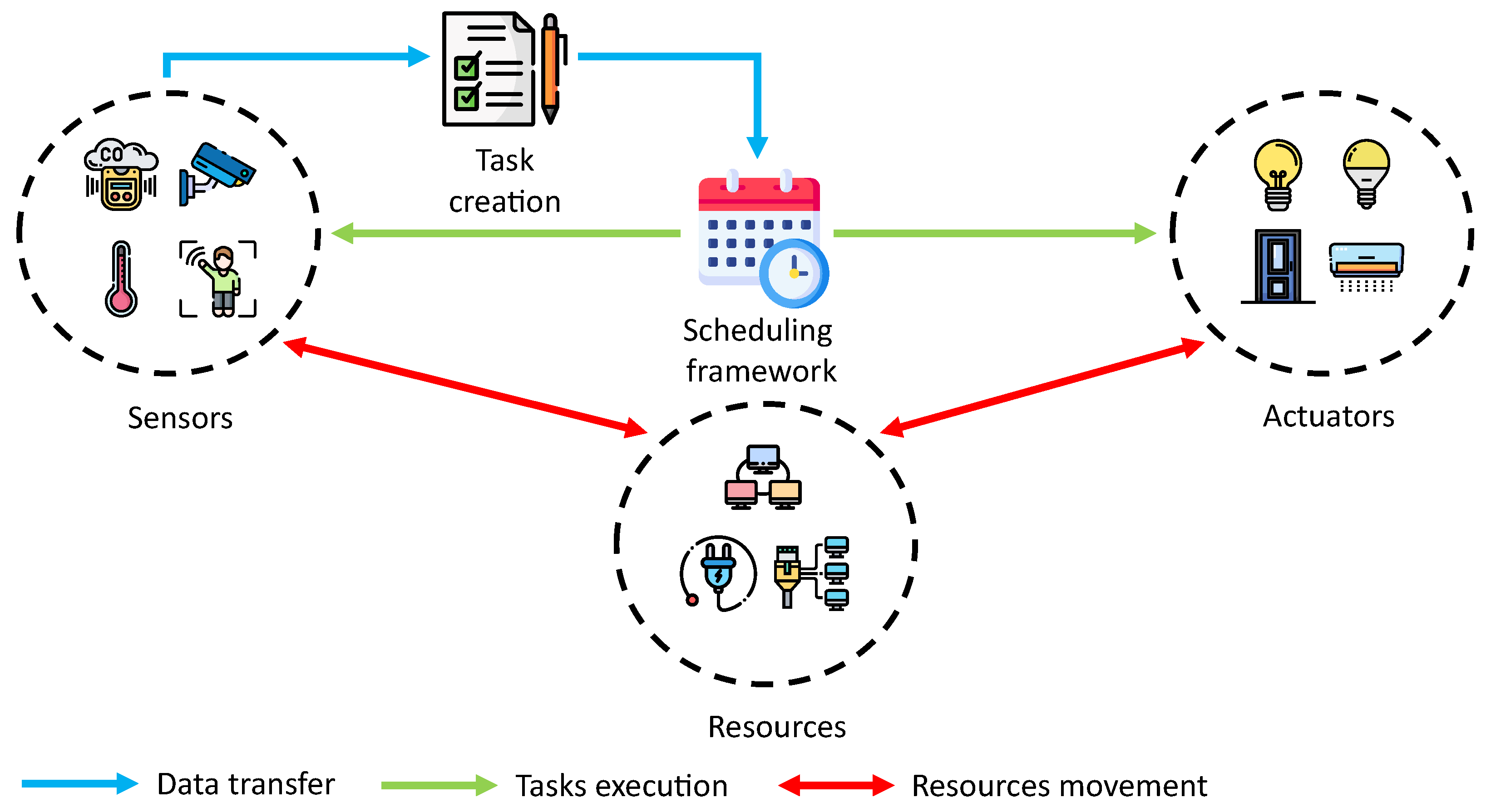
For example, let us consider a smart office system where the resource constraints are the electricity and the data bandwidth between the internal and external servers shown in Figure 1. Based on the sensors’ reading, the task creation dictates the active devices and creates the tasks based on the predefined rule. Then, the scheduling framework creates a scheduler that dictates the time for the sensors and actuators to execute the tasks while ensuring the total resources taken do not exceed the resource constraints. The scheduling framework stores the value of the resources available to keep track of the remaining resources taken by the tasks. The number of active devices and the scheduler’s computation deadline changes according to the number of people inside the building.
In a situation where the number of active devices is not changing, the system designer can implement a scheduling algorithm with high optimization such as Octasort and Fit (OnF) or Sort and Fit (SnF) when the computation deadline is longer. Opposite to this, the system designer can implement a scheduling algorithm with fast computation time such as FCFS or Shortest Job First (SJF) when the computation deadline is shorter. However, in a smart office system where the number of tasks and computation deadline are always changing, OnF or SnF scheduling algorithms cannot meet the computation deadline when scheduling a large number of tasks and resources with a shorter computation deadline. It is the same for the FCFS or SJF, where it cannot create an optimized scheduler when scheduling a large number of tasks and resources with a prolonged computation deadline.
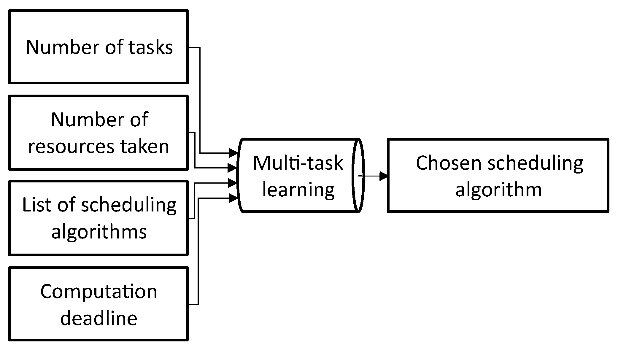
The reason why multiple scheduling algorithms are needed is because each has its trade-off in scheduler optimization and computation time. Inability to meet the requirement will lower down the user satisfaction [6]. This journal proposes a method of Task Scheduling Switcher (TSS)-based multi-task learning (MTL) that is shown in Figure 2 to pick the scheduling algorithm on the fly for the scheduling framework to create a scheduler with the best task execution sequence optimization under the computation deadline.
What makes our proposal better is the MTL’s ability to maintain high accuracy in classifying the best scheduling algorithm by profiling each of the scheduling algorithm’s computation times on the hardware used to compute the scheduler for the system. The previous research [7,8] proved the MTL model’s ability in extracting useful features to increase the classification accuracy in a heterogeneous environment. High classification accuracy in a heterogeneous system is crucial because the system designer cannot guarantee the next IoT system will use the same number of devices, resources, and hardware specifications used to create the scheduler due to the difference in IoT system planning. With the MTL-based TSS implementation on the scheduling framework, we can create a scheduling method with a flexible optimization that is proven to have better optimization, due to the adaptability, than the fixed scheduling algorithm method [9]. With an optimized scheduler available under the computation deadline, it can guarantee quick handling against anomalies in Multiple IoT scenarios (MIoT) [10], and user’s preferences and satisfaction in Social IoT (SIoT) [11].
The main challenge we met in developing the TSS is finding the parameters to observe in deciding the scheduling algorithm, creating a machine learning model that can operate in real time while providing high accuracy and a countermeasure when TSS picked a wrong scheduling algorithm. We settle on the number of tasks and resources taken because it hugely affects the scheduler computation time, and it is the only values that are readily available without analyzing the content of the tasks to reduce the TSS processing time. Then, we use an MTL model due to high classification accuracy in identifying the suitable scheduling algorithm in real time compared to a feedforward neural network (FNN) model [12]. Meanwhile, to ensure that a scheduler is available before the computation deadline, even if the TSS chooses the wrong scheduling algorithm, we implemented a fallback scheduling algorithm to run parallel to TSS.
After the introduction in Section 1, in Section 2, we give the preliminary on the scheduling algorithms and MTL and compare our research with previous research performed on real-time scheduling. In Section 3, we define the task scheduling switcher problem, introduce our proposed design for the MTL model, and the scheduling framework implementation. In Section 4, we evaluate the post-trained MTL model and the scheduling framework on the synthetic benchmark. In Section 5, we implement the scheduling framework on a smart office simulation to simulate near real-life IoT system implementation. Finally, we conclude the works we have carried out and our future planning for this research.
2. Related Work
2.1. Scheduling Algorithm
In this journal, we only implemented four existing scheduling algorithms that show various trade-offs. Although we can use more than four scheduling algorithms depending on the hardware computation specification, we focus on well-known algorithms with our previously proposed algorithm to demonstrate the TSS effectiveness.
Table 1 shows the performance of the four algorithms, i.e., First Come First Serve, Shortest Job First, Sort and Fit and Octasort and Fit observed from our experiment. For example, SJF has fast computation time with low optimization, OnF has slow computation time with high optimization, SnF [13] has a good balance in computation and optimization. In this journal, the scheduling algorithms applied in the experiment are non-preemptive versions.
The scheduler’s computation time and the task execution optimization were calculated by using the Equations (1) and (2). The x represents the computation time to create the scheduler, and represents the OnF’s computation time. Meanwhile, the y represents the scheduler duration to finish all the tasks, and represents the FCFS’s scheduler duration.
FCFS is a scheduling algorithm based on the First In First Out method where the tasks are scheduled based on the task’s scheduling request that arrived first [14]. Although it has fast computation time, it has no task execution optimization.
SJF is a scheduling algorithm that prioritizes the task with the shortest burst time to be executed first. The advantage of this scheduling algorithm is it has a short amount of process average waiting time and turnaround time. It has a slightly faster computation time than FCFS with medium optimization. It is due to our implementation of the SJF scheduling function that needs to check the available resources less frequently than FCFS.
SnF is a scheduling algorithm that sorts the tasks in ascending order based on the burst duration and the number of types of resources taken. Then, based on the sorted order, it executed as many tasks as the resources available allow. If the next one cannot run given the resources available, the algorithm will skip the task. It has medium computation time and high optimization.
OnF is an expanded version of SnF where it sorts the tasks in ascending and descending order and performs the fit operation to create the scheduler. It has the slowest computation time but the highest optimization.
2.2. Multi-Task Learning
MTL works by sharing representations between layers to take advantage of the domain-specific information contained in the training signals of related tasks to ease the classification [15]. MTL is useful in several applications. Zhang et al. [16] proposed the use of MTL for feature extraction. MTL was utilized for feature extraction for downstream tasks such as processing power settings or logarithmic orders of machining stages. Han et al. [17] proposed a rapid sorting method based on multi-task deep learning. They showed that for complex sorting such as visual-sorting, they can improve the efficiency of time while ensuring accuracy and reliability in complex scenarios. Therefore, MTL is a promising method for conducting multiple learning tasks applicable to the sorting and scheduling approach.
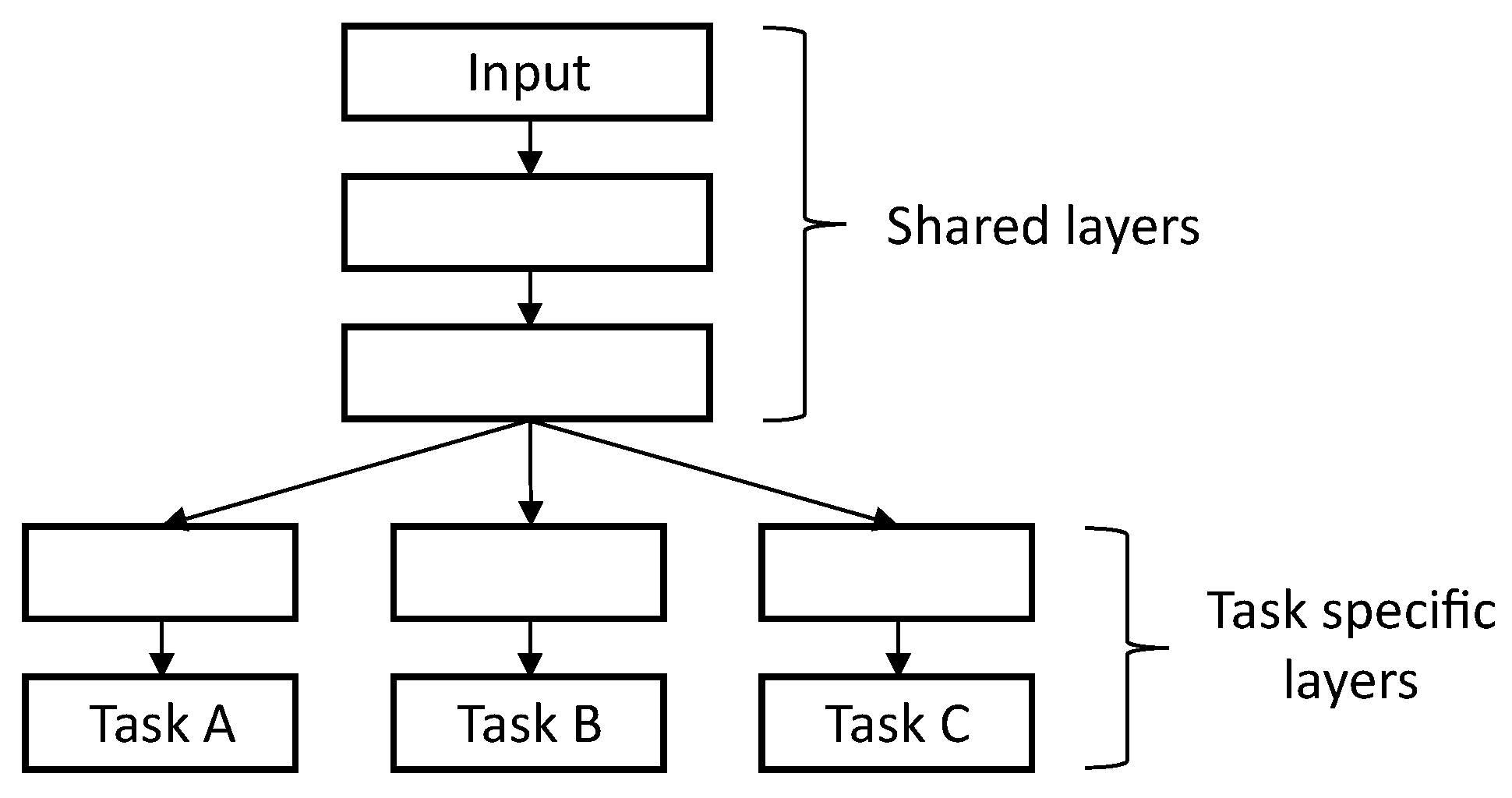
In this journal, we use hard parameter sharing for MTL to identify the best scheduling algorithm. Figure 3 illustrates the multi-task learning consists of different layers such as shared layers and task-specific layers. The learning task was separated into different tasks, i.e., Task A, Task B, and Task C.
2.3. Previous Research
In [13], we proposed a new scheduling algorithm called Sort and Fit as part of an IoT platform called Elgar platform, which adopts the concept of “Design Once, Provide Anywhere” [18]. It supports the implementation of heterogeneous devices based on one universal service design where any device that is compatible with the configuration can process the task according to the scheduling algorithm. Although SnF has a better balance in average computation time and optimization, the brute force or FCFS scheduling algorithm yields better results in certain situations. For this reason, it makes SnF less viable when the number of tasks and resources taken along with the computation deadline are always changing.
Heger et al. [19] proposed an online-scheduling approach that utilizes the past and real-time data to improve the performance of the manufacturing system. Their result shows that their approach can improve the system performance that has higher fluctuations.
Jiang et al. proposed a new method based on federated scheduling that can perform better when scheduling the parallel task under a tight deadline [20]. Their experiment result shows it can outperform the previously proposed methods, specifically for the task sets consisting of tasks with a tight deadline.
Wu et al. proposed real-time scheduling based on deep reinforcement learning to schedule a large production number of medical masks [21]. Their randomized simulation results show their method can solve the scheduling problem within 1–2 s.
As shown in Table 2, although all the scheduling algorithms can compute in real time, not all can optimize the task execution inside the scheduler. Furthermore, no algorithm offers flexible optimization according to the computation deadline. Our proposed TSS gives the edge against the previously proposed scheduling algorithm by switching the scheduling algorithm with higher optimization with a prolonged computation deadline.
3. Modeling the Task Scheduling Switcher
3.1. Task Scheduling Switcher Problem
As previously shown in Figure 2, which shows the overview of the TSS, the MTL selects an algorithm from the set of scheduling algorithm FCFS, SJF, SnF, OnF} for the scheduling algorithm to choose based on the normalized value of the number of tasks , the number of resources taken , and the computation deadline using the min–max normalization method. From there, we can define the input and output problem for the TSS as shown in Problem 1.
Problem 1
(Problem in Choosing the Scheduling Algorithm).
Input: FCFS, SJF, SnF, OnF} and the parameters to schedule the tasks , , .
Output: {FCFS, SJF, SnF, OnF} expected from the TSS.
3.2. Multi-Task Learning Model
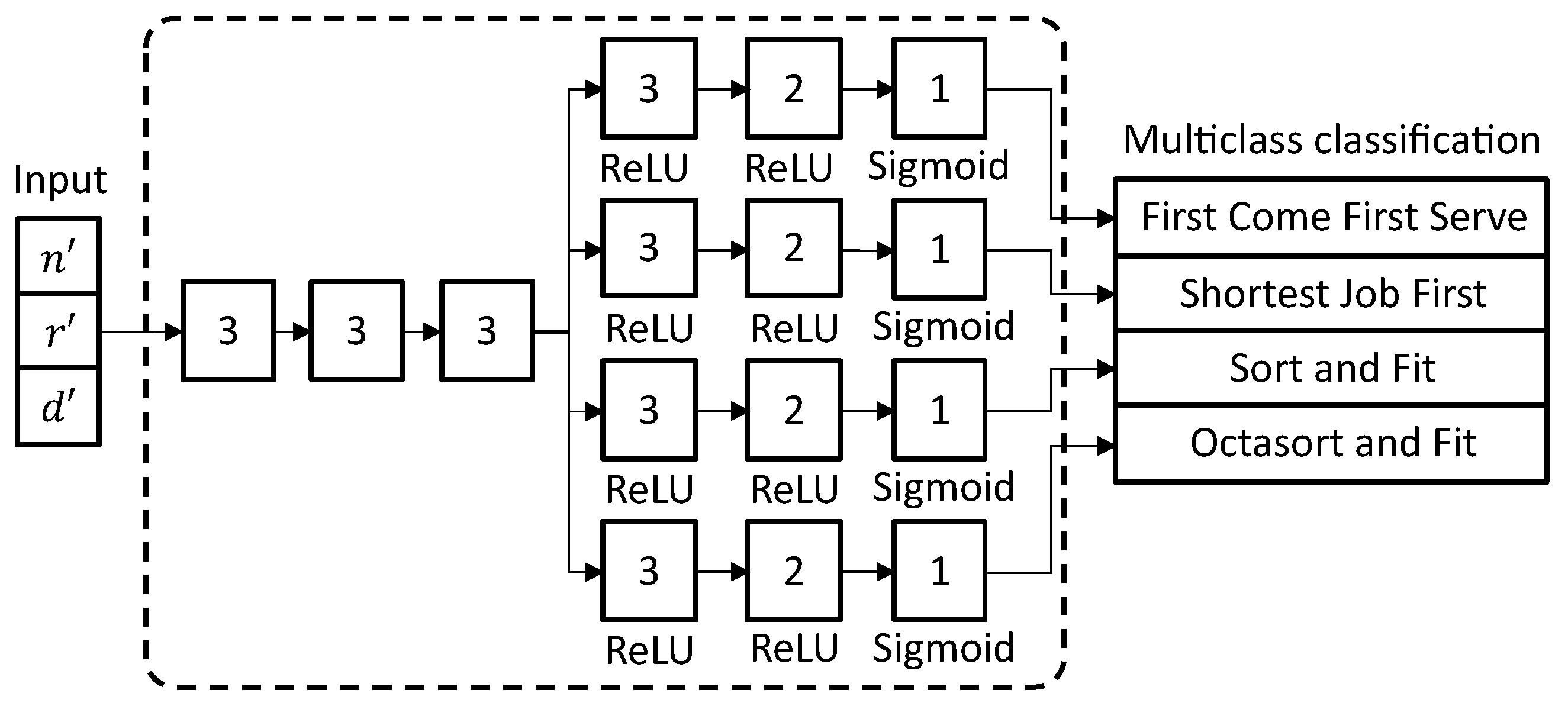
We implement the TSS as an MTL model where the input consists of the normalized value of , , and using the min–max normalization method to rescale the values in the range of 0 to 1 to improve the learning rate [22]. As shown in Figure 4, the smaller box represents the layer inside the model, the number inside the box represents the number of the node, the text under the boxes represents the activation function for each layer. The first three layers connected to the input act as a shared layer; the rest of the branched layers act as a task-specific layer. Although the first two of the task-specific layers have an activation function of a rectified linear unit (ReLU), the final layer has an activation function of Sigmoid. We implement the MTL model on the TensorFlow machine learning library [23] shown in Listing A1. To compile the model, we use Adam as an optimizer, binary cross-entropy with a similar loss weight value, as combined loss and accuracy, as the metric shown in Listing A2.
The MTL model compiled with TensorFlow with 3000 epoch and 1000 batch size for training the dataset with 100,000 labeled data split to for training and for the test following the parameters shown in Table 3. We used the TensorFlow’s built-in “ModelCheckpoint” callback function [24] to save the MTL model with the lowest validation combined loss and the “EarlyStopping” callback function [25] to stop the training when the model could no longer improve the accuracy.
After the training and the MTL model are deemed to have good accuracy when validated on the test dataset, we optimize the MTL model using a post-training quantization [26] to reduce the model size and interfacing latency, albeit with a little trade-off in model accuracy. Quantization of the MTL model works by converting the weight that controls the signal between the two nodes from 32-bit float precision to a type with lower precision (16-bit floats or 8-bit integers) for faster arithmetic operation. The reason for the trade-off of using quantization is due to lower accuracy in the floating-point arithmetic.
In this journal, we use dynamic range quantization to optimize the model by quantizing the weights to an 8-bit integer. TensorFlow quantizes the MTL model activations dynamically based on their range to 8-bit and computes the weights and activations with 8-bit precision [27]. Although the interfacing latency is fast, the speed is still less than a fully fixed-point inference due to the outputs that are stored in floating point.
3.3. Scheduling Framework Implementation
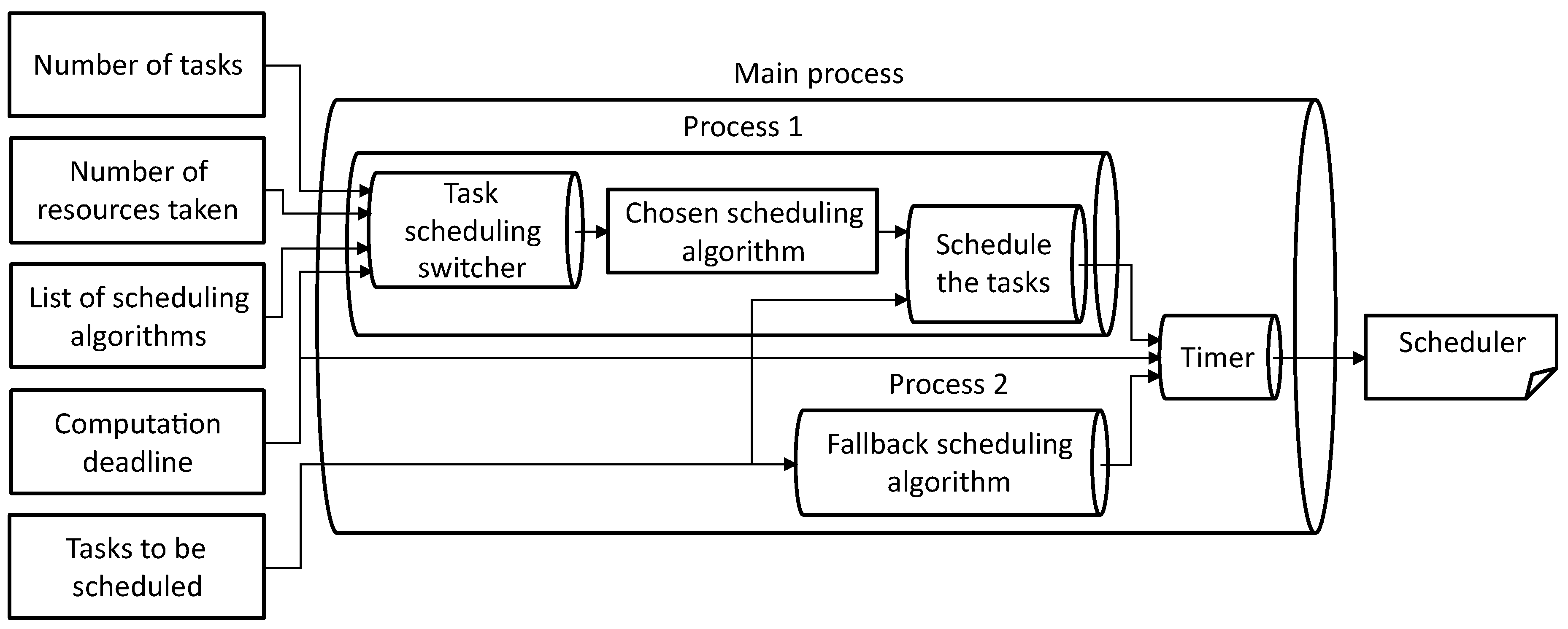
Figure 5 shows an overview of our proposed TSS in the scheduling framework in which Process 1 and Process 2 are the child process of the Main process. In other words, Process 1 and Process 2 are running in parallel. Referring to Process 1, the TSS recommends chosen from FCFS, SJF, SnF, OnF} based on the , , . Then, from the set of scheduling algorithms A, the scheduling framework will switch the scheduling framework with the recommended one and schedule the tasks to be scheduled to create a scheduler where , execution time . From there, we can define the input and output problem for the TSS implementation shown in Process 1.
Process 1
(Task Scheduling Switcher Based Scheduling Framework).
Input:, , , FCFS, SJF, SnF, OnF}, .
Output:Process 1 scheduler.
If TSS on Process 1 cannot create the scheduler under the computation deadline, the scheduling framework will use the scheduler from the fallback scheduling algorithm on Process 2. The fallback scheduling algorithm uses a scheduling algorithm with the lowest computation time for ensuring high chances of meeting the computation deadline. By referring back to Table 1, the scheduling algorithm with the shorter computation time is SJF. From there, we can define the input and output for the fallback scheduling algorithm shown in Process 2.
Process 2
(Fallback Scheduling Algorithm to Backup the Process 1).
Input:.
Output:Process 2 scheduler.
In the Main process, the Timer chooses the scheduler either from Process 1 or Process 2 based on the remaining time before the computation deadline. If Process 1 manages to compute the scheduler before the deadline, the Timer chooses the scheduler from Process 1. Otherwise, if Process 1 cannot complete the computation before the computation deadline, the scheduler from Process 2 is used. Otherwise, if both processes could not compute the scheduler under the computation deadline, the first process that completed the scheduler computation is used instead.
4. Evaluation
4.1. Hardware Specification
In this journal, we use the notebook computer with the specification shown in Table 4 where the programming environment used is Anaconda Individual Edition [28] with preinstalled base environment which holds Python . Then, we added TensorFlow GPU version and CUDA Toolkit [29] to the base environment.
4.2. Classification Accuracy
4.2.1. Dataset Creation
To test our proposed MTL model, we must create a large dataset with equal labeling on the scheduling algorithm chosen. To prevent bias, we created a large dataset where the labelings for the scheduling algorithms are balanced.
Algorithm 1 shows the pseudocode to create the dataset with 100,000 of equally labeled data. The represents the random seed value to get a replicable result, and the seed() is the function to initialize the pseudorandom number generator. Meanwhile, represents the randomization ranges for the number of tasks, resources to be taken, and the amount taken. After initializing the value of and the empty list of to store the dataset, the program will call the dataCreation() function for 25,000 times where each time the dataCreation() was called, it will create four labeled data to be saved temporarily in the before being saved in . The reasoning for four labeled data is due to each of the data corresponding to the scheduling algorithm used in this journal.
| Algorithm 1 Creating a dataset for training the MTL model. |
|
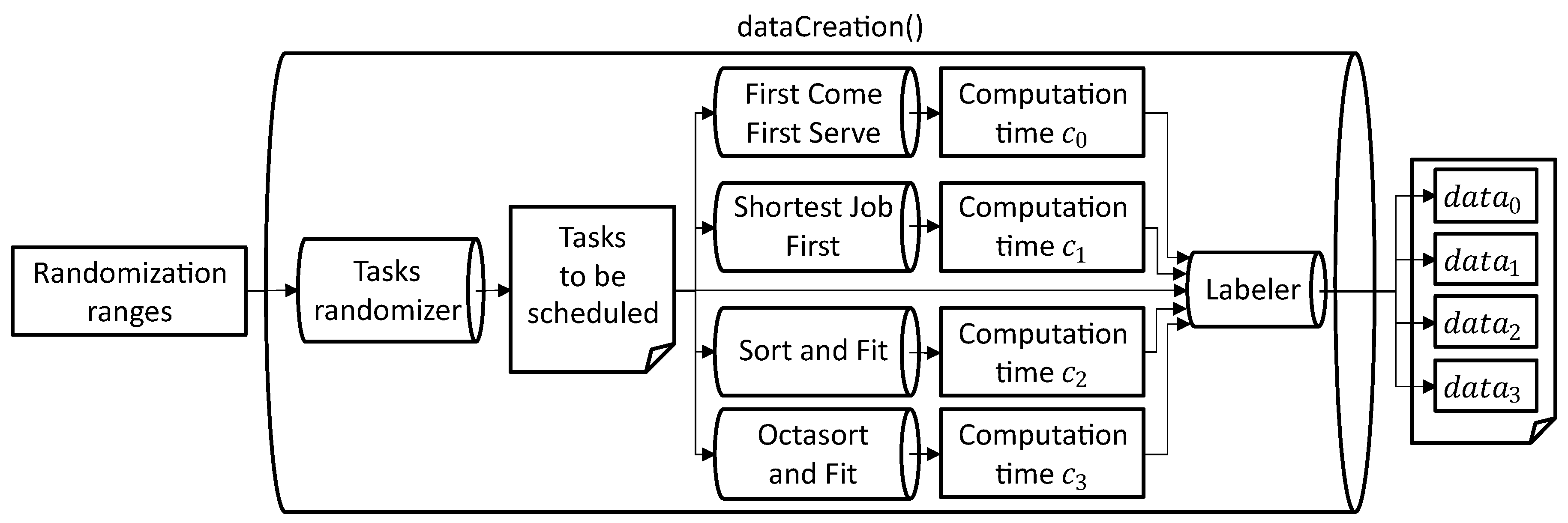
Figure 6 shows the context diagram of dataCreation() operation. Based on the randomization ranges , , , the range for the tasks is , range for the number of resources taken by the tasks , and range for each resource constraint where dictate the controlled randomization of the tasks to be scheduled. Then, the randomized tasks are computed by each of the scheduling algorithms in sequence to get the computation time where is the computation time for FCFS, is SJF, is SnF, and is OnF. Based on the recorded computation time, the set of the computation deadline D is randomized following Property 1.
Property 1
(Set of computation deadline D).
Consider a set of recorded computation time where the values are . Set of computation deadline can be defined as , , , and . □
Finally, we can define the dataCreation() function as , , , where the , . While represents the input data to be fed into the MTL model, represents the data that the MTL model is expected to output. We generated the dataset by using the randomization ranges specified in Table 5.
4.2.2. Post-Training Log
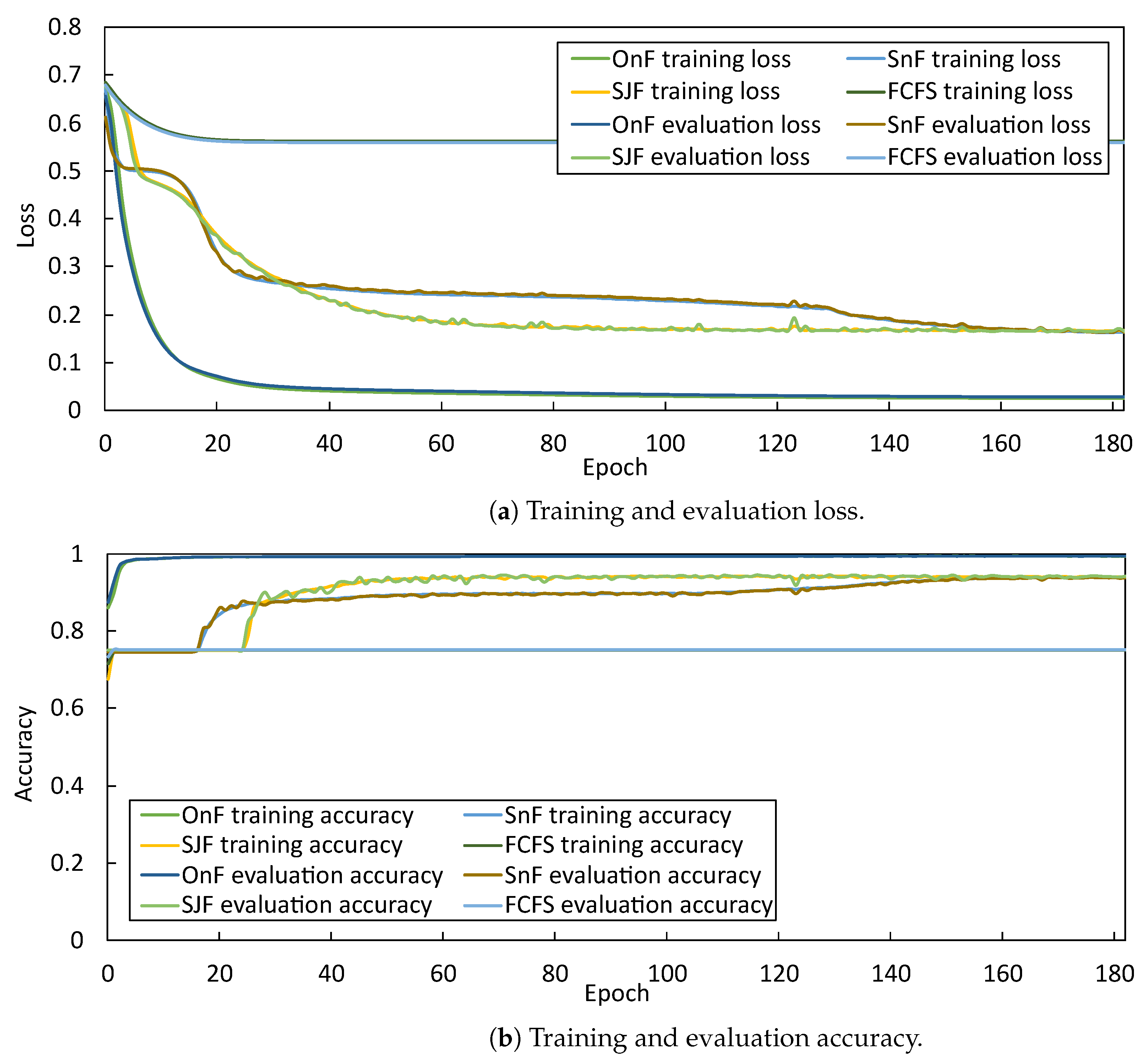
After training the MTL model on epoch 182, it gets , , , and of loss in choosing FCFS, SJF, and SnF. Meanwhile, for the evaluation loss, the model gets , , , and as shown in Figure 7a. The combined loss for the model is . Moving on, the MTL model gets , , , and of accuracy in choosing FCFS, SJF, SnF, and OnF. Meanwhile, for the evaluation accuracy, the model gets , , , and as shown in Figure 7b.
The figures that recorded the post-training log of the MTL model represent the learning curves of the exponential fall and rise to limit for Figure 7a,b. From there, we know the MTL model effortlessly retains the necessary information to classify the scheduling algorithm during the initial epochs before the rate falls into a constant. In other words, the MTL model requires shorter epoch numbers to have high accuracy in classifying the correct scheduling algorithm. Based on the shape of the learning curves and how the training and evaluation lines overlap each other for loss and accuracy, the MTL model does not suffer from the overfitting problem [30].
4.2.3. Cross-Validation Results
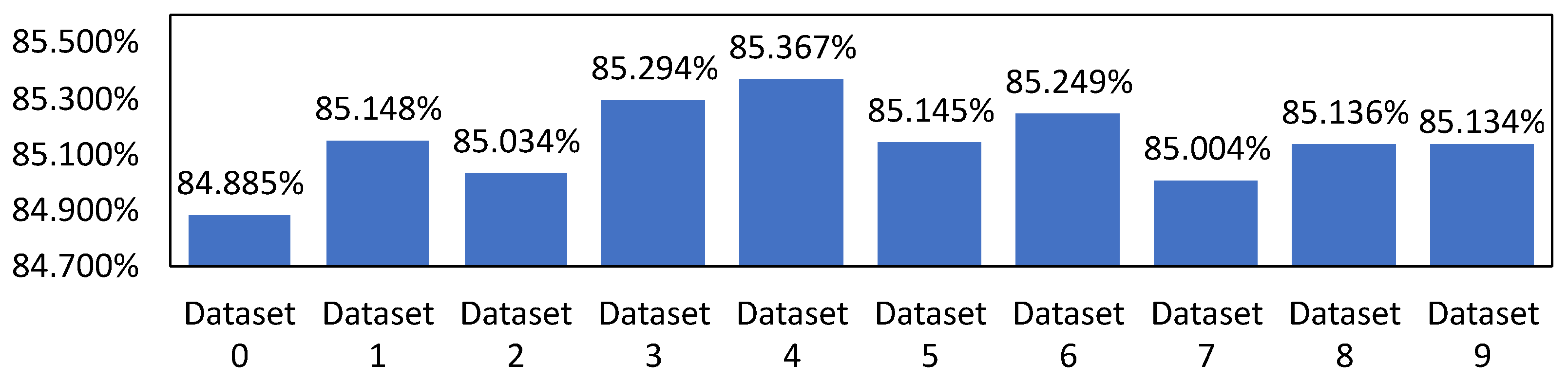
We performed cross-validation on ten new datasets not used to train the MTL model to validate the model’s accuracy in classifying the scheduling algorithm. Figure 8 shows that the model has an accuracy of above in choosing the scheduling algorithm with the best optimization plausible under the computation deadline. On average, it has an average accuracy of , which shows how effective the model is.
4.3. Benchmarking the Scheduling Framework
4.3.1. Benchmark Configuration
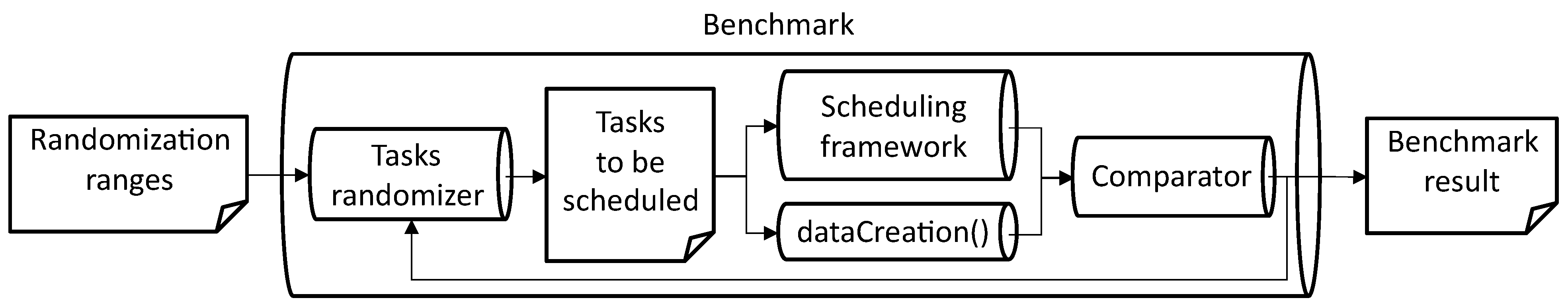
To evaluate our implementation of the scheduling framework, we create a benchmarking program to perform a stress test shown in Figure 9. Firstly, the benchmarking program creates a new set of tasks to be scheduled and process it with scheduling framework and dataCreation() in sequence. Then, the Comparator judges the accuracy of scheduling framework in meeting the computation deadline and the optimization percentage and compare it with the labeled data. This process repeats for 2500 times.
4.3.2. Benchmark Result
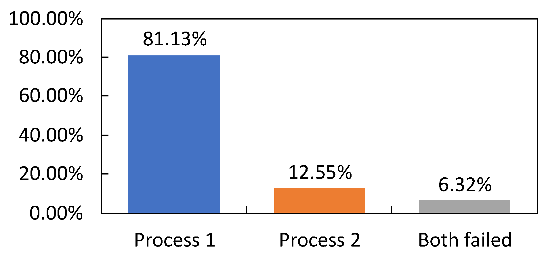
Figure 10 shows the relationship between Process 1 and Process 2 analyzed by the Comparator. From the result shown, we know the scheduling framework has an average of using the scheduler from Process 1 for and Process 2 for . In other words, Process 1 was able to meet the computation deadline to create the scheduler for an average of , while in the cases where Process 1 failed to meet the computation deadline, the scheduling framework used the scheduler generated by Process 2 where Process 2 has an average of meeting the computation deadline for an average of .
Comparing the scheduler generated by Process 1 that was able to meet the computation deadline with the result shown in Figure 8, we confirmed the average processing latency added by the TSS is negligible, which is 30.891 μs as measured by our benchmarking program. Our model has low processing latency, albeit the computational complexity for MTL is higher than FNN due to the fact that the proposed MTL model design has fewer nodes connecting between each layer. Furthermore, the dynamic range quantization also speeds up the computation by performing the calculation with lower precision.
Although with the implementation of Process 2 as the fallback scheduling algorithm to ensure a backup scheduler is available when Process 1 failed to meet the computation deadline, the benchmark result shows that our scheduling framework implementation has an average of for both processes unable to meet the computation deadline. In other words, in a situation where Process 1 is unable to create the scheduler under the computation deadline, there is a chance of Process 2 being unable to provide a backup scheduler. In this situation, the scheduling framework uses the scheduler from either Process 1 or 2 that completed the scheduler creation first. This behavior is due to Process 2 being assigned on the CPU core where the background tasks running on it affect the computation time.
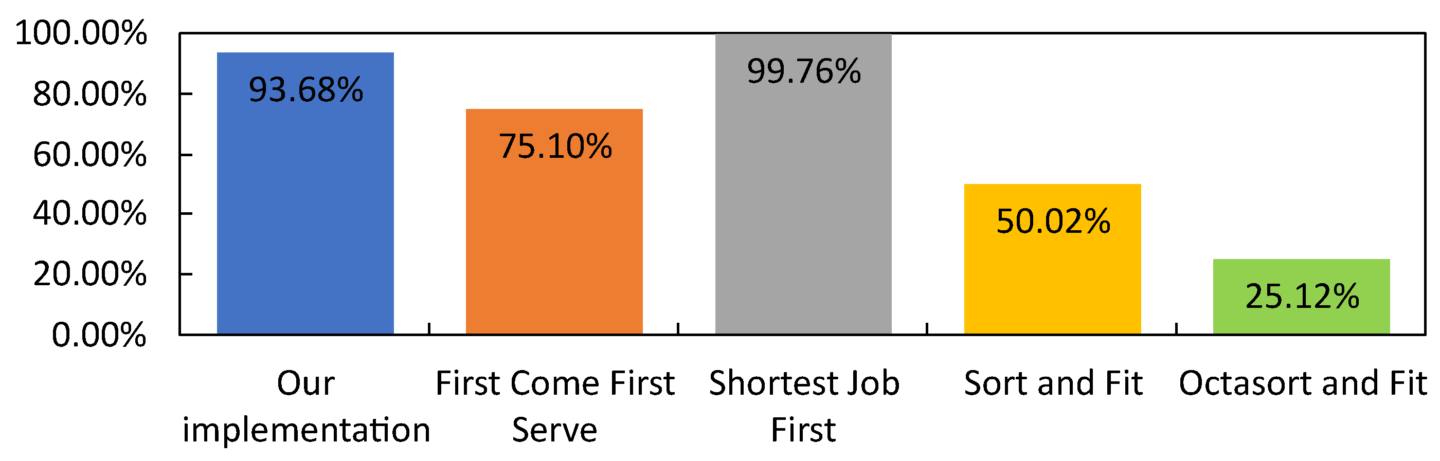
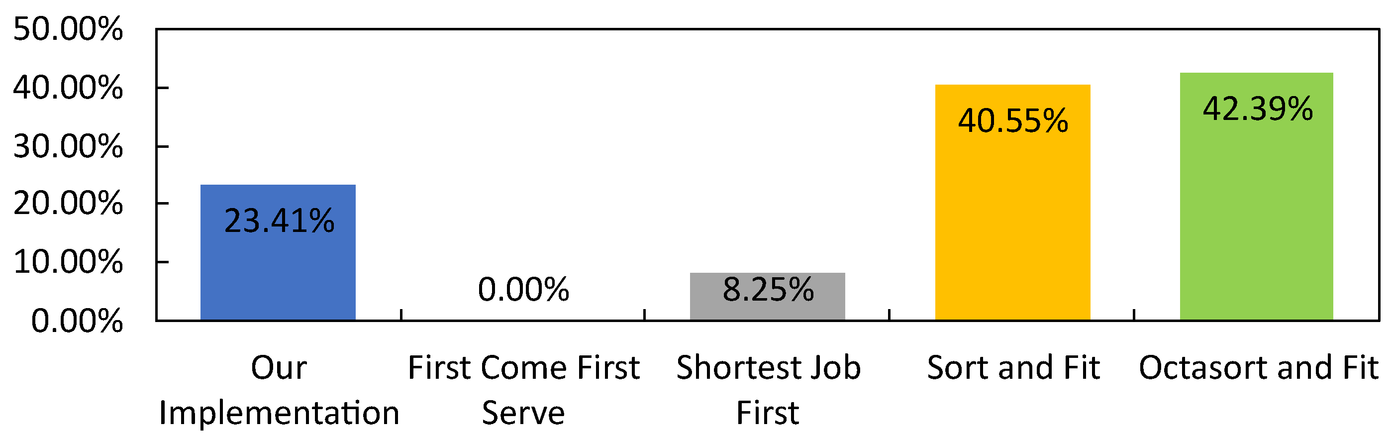
Figure 11 shows that our implementation has an average accuracy in meeting the computation deadline of . The only scheduling algorithm with the highest average accuracy in meeting the computation deadline is SJF, followed by our implementation, FCFS, SnF, and OnF. Although the result shows that SJF is better than our implementation in meeting the computation deadline, Figure 12 shows that SJF has the worst average optimization with FCFS as a base reference. Meanwhile, our implementation has an average of of optimization. Our results show that our implementation has good accuracy in meeting the computation deadline and scheduler optimization compared to the scheduling framework that only uses a single scheduling algorithm.
5. Validation
5.1. Simulating the Resource-Constrained Smart Office
To validate the effectiveness of our proposed TSS implementation on the scheduling framework, we simulate a medium-sized smart office building [31] system that is in the middle of upgrading the electrical power delivery with the internet connection. The system resources became constrained due to a decrease in system infrastructure. It makes single scheduling algorithm harder to find the best task execution arrangement to fit the available system resources under the computation deadline. With the increases in complexity of the scheduling problem, we expect that the TSS can optimize the scheduler before the computation deadline by switching the scheduling algorithm depending on the number of people inside the building. To ensure that the simulation model is close to the real-world problem, we only randomized the number of tasks and their duration. Meanwhile, the maximum number of active types of devices, the resources taken to execute the tasks, resource constraints, and the number of people inside the building follow the simulation rule defined in the next section.
5.2. Simulation Configuration
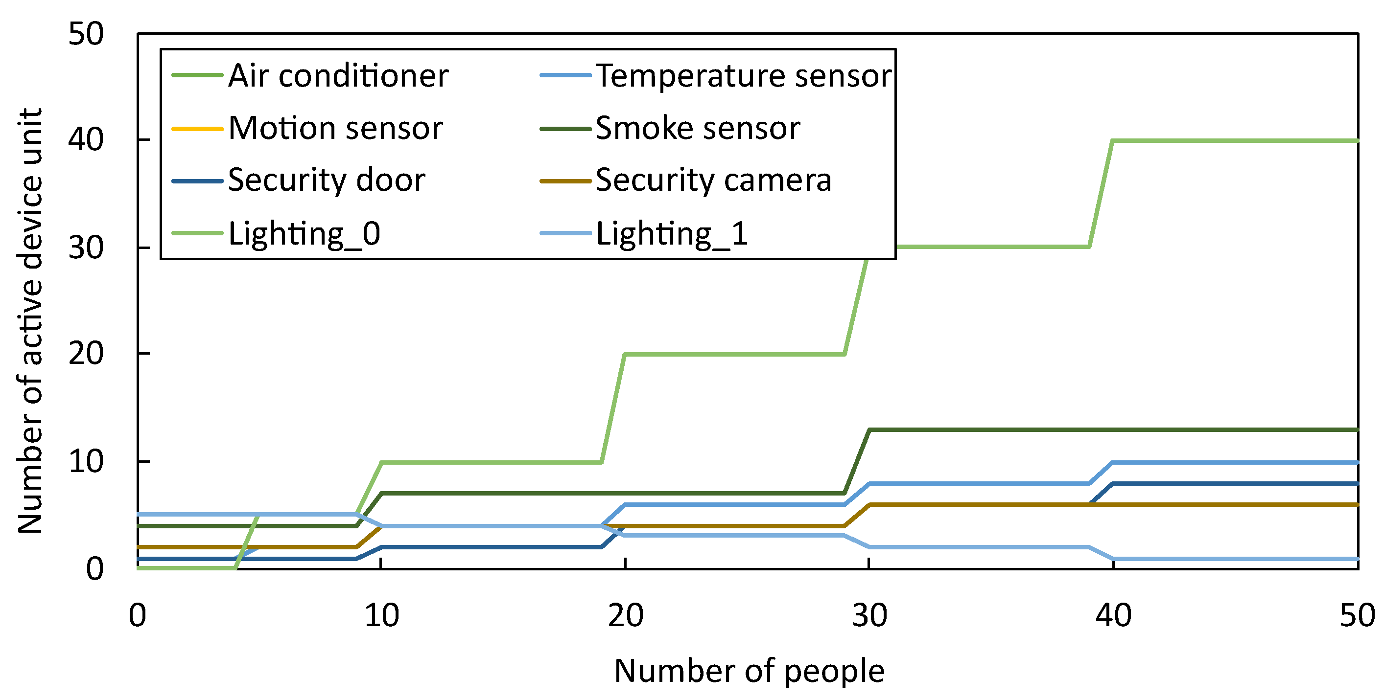
We simulated a smart office building system to schedule the IoT device units shown in Table 6, where a different number of units are installed and the number of resources consumed. The resources that act as a bottleneck in this system are the electricity and connectivity bandwidth for the local area network (LAN) and the wide area networks (WAN). For this simulation, the electricity constraint is 5000 W, the LAN constraint is 50 MB/s, and the WAN constraint is 100 MB/s. We configured the resource constraints large enough where only a small degree of optimization is plausible to make it hard to optimize the scheduler without choosing the correct scheduling algorithm. Based on the hourly number of people shown in Figure 13, the number of active device unit changes according to the activation rule shown in Figure 14.
Meanwhile, we dictate the computation deadline to change according to the number of people inside the building to provide a satisfying service. In Equation (3), represents the best-case time complexity of the fastest scheduling, represents the worst-case time complexity of the slowest scheduling algorithm, and represents the number of people. In the simulation, the value of the is s and the value of the is s. Based on these parameters, a new training dataset is randomized and used to train the same MTL model with no changes in training parameters previously used in the evaluation.
Finally, the unit’s task duration is randomized in the range of 0.1s to 100s, while the number of scheduled device units needed is randomized between 0 and the max active number of device units.
5.3. Simulation Result
5.3.1. Sampled Scheduling Algorithm Switching
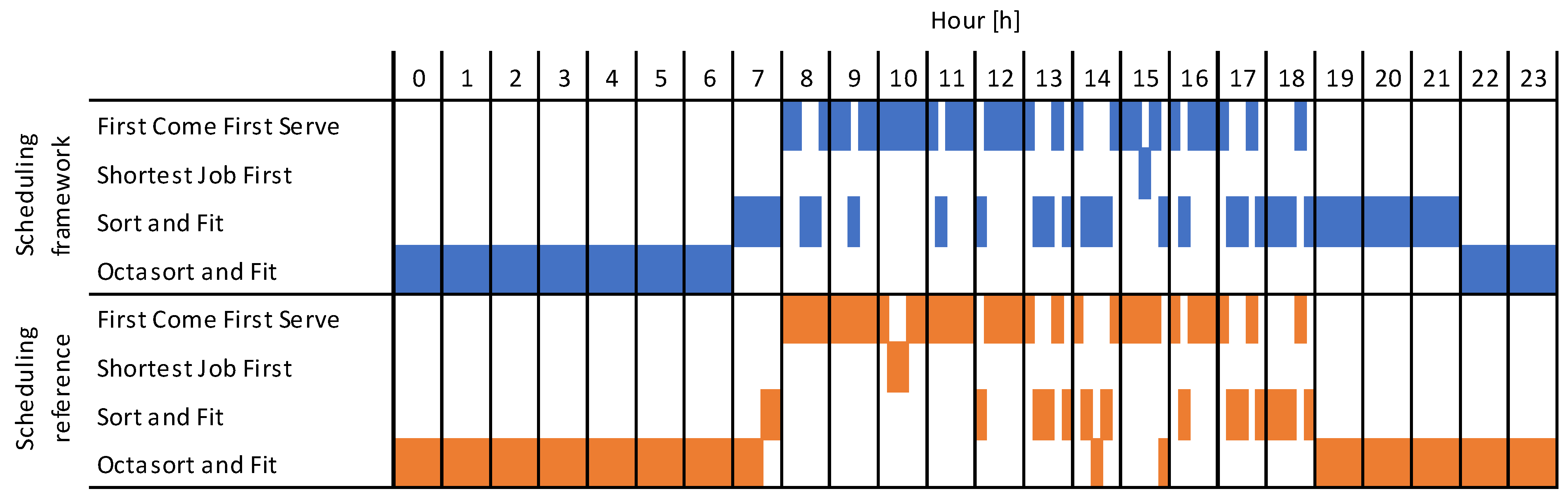
Figure 15 shows the comparison between the TSS-based scheduling framework with the correct scheduling algorithm switching called scheduling reference. To simplify the Gantt chart representation, we sampled the hourly result of the scheduling algorithms switching to five times from the original 1000 simulation data in one hour. As we can see, TSS leans toward the OnF scheduling algorithm with a low number of people, while TSS leans toward the FCFS with a high number of people. In other words, as the number of people inside the building increases, the scheduling algorithm chosen by the TSS changes from the longest computation time to the shortest computation time.
Although the Gantt chart for the scheduling framework and scheduling reference is almost similar, the plotted chart is slightly different at the peak hours. As we can see the chosen scheduling algorithm at 0800, the scheduling framework picked SnF 2 times out of 5 instead of FCFS. Referring back to Table 1, this is due to the close computation time taken by the OnF and SnF. By taking the average 24,000 scheduling result for one day, TSS classification accuracy is , which is lower than the classification accuracy we had from the benchmark result.
5.3.2. Deadline Accuracy and Optimization
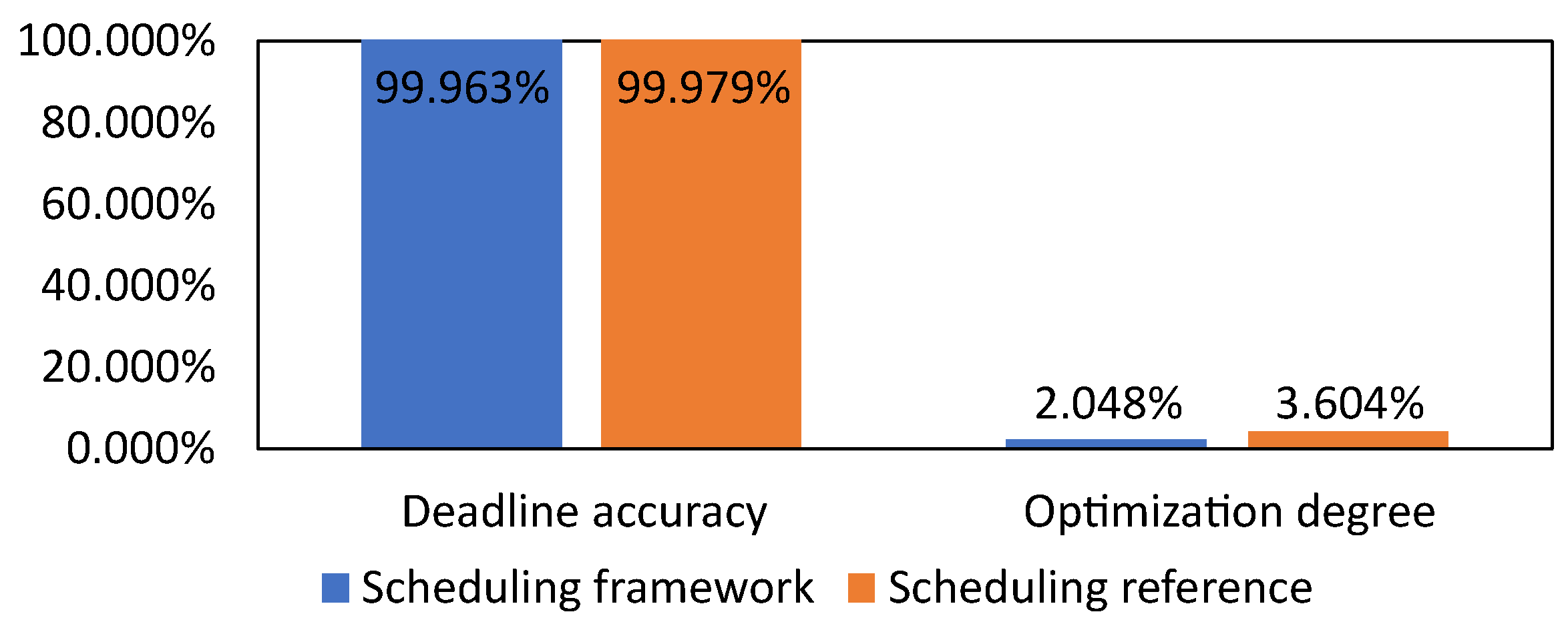
Figure 16 shows the average deadline accuracy and optimization degree calculated from 24,000 scheduler data. With the help of fallback scheduling algorithm implementation in the scheduling framework, it guaranteed almost of computation deadline accuracy. Furthermore, with resource constraints on the electricity and bandwidths not being small enough, the optimization degree on scheduling reference and scheduling framework is low, matching our configuration.
5.4. Discussion
Referring to the hourly number of people inside the building shown in Figure 13, the behavior of the TSS in picking the scheduling algorithm matches our expectation; whereas the number of people increases, TSS leans more toward the scheduling algorithm with the shortest computation time to meet the computation deadline. The computation deadline window shown in Equation (3) is not as tight as the benchmark program, where the computation deadline is randomized in a small margin. With more room in the computation deadline, SJF picked less than FCFS due to SJF has faster computation time than the FCFS. This result aligns with our expectations, where TSS prioritizes the computation deadline accuracy before the scheduling optimization.
Meanwhile, the TSS accuracy of identifying the correct scheduling algorithm would be low compared to the accuracy we obtained in Figure 8. With a system configuration with a low number of resource constraints, it becomes harder for the MTL to classify the correct scheduling algorithm due to the small number of resources that do not significantly affect the computation time. Furthermore, the noise added from the background operating system processes running during the simulation also influences the computation time, making things worse.
6. Conclusions
We explore the viability of using MTL to switch the scheduling algorithm in real time to achieve the best optimization plausible under the computation deadline. In case MTL makes a wrong decision, the implementation of the fallback scheduling algorithm can guarantee an average of of computation deadline accuracy based on our benchmark result. Moreover, our results show that the MTL model has accuracy in classifying the best scheduling algorithm for scheduling the tasks based on the parameters given. Although our smart office simulation shows a minuscule gain in optimization, we got an average of 99.963% computation deadline accuracy; there was 0.016% difference compared to the scheduling reference.
For future works, we aim to expand the TSS capability to tackle large-scale distributed scheduling, such as smart city for efficient city resources management, especially during a natural disaster where resources are not only limited to consumables but human resources as well.
Author Contributions
Data curation, M.H.B.K.; Formal analysis, M.H.B.K.; Funding acquisition, S.Y.; Investigation, M.H.B.K.; Methodology, M.H.B.K., M.A.B.A. and S.Y.; Project administration, S.Y. Resources, M.H.B.K.; Software, M.H.B.K.; Supervision, M.A.B.A. and S.Y.; Validation, M.H.B.K.; Writing–original draft, M.H.B.K.; Writing–review & editing, M.A.B.A. and S.Y. All authors have read and agreed to the published version of the manuscript.
Funding
This research was partially supported by Interface Corporation, Japan.
Conflicts of Interest
The authors declare no conflict of interest.
Appendix A

Listing A1.
Proposed MTL model implementation on the TensorFlow machine learning library.
 |
Listing A2.
Parameters used to compile the MTL model.
 |
References
- Yugha, R.; Chithra, S. A survey on technologies and security protocols: Reference for future generation IoT. J. Netw. Comput. Appl. 2020, 169, 1–13. [Google Scholar] [CrossRef]
- Al-Jarrah, M.A.; Yaseen, M.A.; Al-Dweik, A.; Dobre, O.A.; Alsusa, E. Decision Fusion for IoT-Based Wireless Sensor Networks. IEEE Internet Things J. 2020, 7, 1313–1326. [Google Scholar] [CrossRef]
- Ciuonzo, D.; Javadi, S.H.; Mohammadi, A.; Rossi, P.S. Bandwidth-Constrained Decentralized Detection of an Unknown Vector Signal via Multisensor Fusion. IEEE Trans. Signal Inf. Process. Over Netw. 2020, 6, 744–758. [Google Scholar] [CrossRef]
- Hwang, S.I.; Cheng, S.T. Combinatorial Optimization in Real-Time Scheduling: Theory and Algorithms. J. Comb. Optim. 2001, 5, 345–375. [Google Scholar] [CrossRef]
- Jha, H.; Chowdhury, S.; Ramya, G. Survey on various Scheduling Algorithms. Imp. J. Interdiscip. Res. 2017, 3, 1749–1752. [Google Scholar]
- Li, G.; Wu, Y.; Lin, D.; Zhao, S. Methods of Resource Scheduling Based on Optimized Fuzzy Clustering in Fog Computing. Sensors 2019, 19, 2122. [Google Scholar] [CrossRef] [PubMed] [Green Version]
- Aceto, G.; Ciuonzo, D.; Montieri, A.; Pescapé, A. DISTILLER: Encrypted traffic classification via multimodal multitask deep learning. J. Netw. Comput. Appl. 2021, 1–19. [Google Scholar] [CrossRef]
- Leem, S.; Yoo, I.; Yook, D. Multitask Learning of Deep Neural Network-Based Keyword Spotting for IoT Devices. IEEE Trans. Consum. Electron. 2019, 65, 188–194. [Google Scholar] [CrossRef]
- Rafique, M.; Haider, Z.; Mehmood, K.; Zaman, M.S.U.; Irfan, M.; Khan, S.; Kim, C.-H. Optimal Scheduling of Hybrid Energy Resources for a Smart Home. Energies 2018, 11, 3201. [Google Scholar] [CrossRef] [Green Version]
- Cauteruccio, F. A framework for anomaly detection and classification in Multiple IoT scenarios. Future Gener. Comput. Syst. 2021, 114, 322–335. [Google Scholar] [CrossRef]
- Cauteruccio, F.; Cinelli, L.; Fortino, G.; Savaglio, C.; Terracina, G.; Ursino, D.; Virgili, L. An approach to compute the scope of a social object in a Multi-IoT scenario. Pervasive Mob. Comput. 2020, 67, 101223. [Google Scholar] [CrossRef]
- Bebis, G.; Georgiopoulos, M. Feed-forward neural networks. IEEE Potentials 1994, 13, 27–31. [Google Scholar] [CrossRef]
- Kamilin, M.H.B.; Ahmadon, M.A.B.; Yamaguchi, S. Evaluation of Process Arrangement Methods Based on Resource Constraint for IoT System. In Proceedings of the 2020 8th International Conference on Information and Education Technology, Okayama, Japan, 28–30 March 2020; pp. 290–294. [Google Scholar]
- Choudhary, N.; Gautam, G.; Goswami, Y.; Khandelwal, S. A Comparative Study of Various CPU Scheduling Algorithms using MOOS Simulator. J. Adv. Shell Program. 2018, 5, 1–5. [Google Scholar]
- Ruder, S. An Overview of Multi-Task Learning in Deep Neural Networks. arXiv 2017, arXiv:1706.05098v1. [Google Scholar]
- Zhang, Q.; Wang, Z.; Wang, B.; Ohsawa, Y.; Hayashi, T. Feature Extraction of Laser Machining Data by Using Deep Multi-Task Learning. Information 2020, 11, 378. [Google Scholar] [CrossRef]
- Han, S.; Liu, X.; Han, X.; Wang, G.; Wu, S. Visual Sorting of Express Parcels Based on Multi-Task Deep Learning. Sensors 2020, 20, 6785. [Google Scholar] [CrossRef] [PubMed]
- Ahmadon, M.A.B.; Yamaguchi, S.; Mahamad, A.K.; Saon, S. Physical Device Compatibility Support for Implementation of IoT Services with Design Once, Provide Anywhere Concept. Information 2021, 12, 30. [Google Scholar] [CrossRef]
- Heger, J.; Grundstein, S.; Freitag, M. Online-scheduling using past and real-time data. An assessment by discrete event simulation using exponential smoothing. CIRP J. Manuf. Sci. Technol. 2017, 19, 158–163. [Google Scholar] [CrossRef]
- Jiang, X.; Guan, N.; Long, X.; Tang, Y.; He, Q. Real-time scheduling of parallel tasks with tight deadlines. J. Syst. Archit. 2020, 108, 101742. [Google Scholar] [CrossRef]
- Wu, C.X.; Liao, M.H.; Karatas, M.; Chen, S.Y.; Zheng, Y.J. Real-time neural network scheduling of emergency medical mask production during COVID-19. Appl. Soft Comput. 2020, 97, 106790. [Google Scholar] [CrossRef]
- Singh, D.; Singh, B. Investigating the impact of data normalization on classification performance. Appl. Soft Comput. 2020, 97, 105524. [Google Scholar] [CrossRef]
- Abadi, M.; Agarwal, A.; Barham, P.; Brevdo, E.; Chen, Z.; Citro, C. TensorFlow: Large-scale machine learning on heterogeneous systems. In Proceedings of the 12th USENIX Symposium on Operating Systems Design and Implementation (OSDI ’16), Savannah, GA, USA, 2–4 November 2016; pp. 265–283. [Google Scholar]
- tf.keras.callbacks.ModelCheckpoint. TensorFlow. 14 December 2020. Available online: www.tensorflow.org/api_docs/python/tf/keras/callbacks/ModelCheckpoint (accessed on 20 December 2020).
- tf.keras.callbacks.EarlyStopping. TensorFlow. 13 January 2021. Available online: www.tensorflow.org/api_docs/python/tf/keras/callbacks/EarlyStopping (accessed on 18 January 2021).
- Jacob, B.; Kligys, S.; Chen, B.; Zhu, M.; Tang, M.; Howard, A.; Kalenichenko, D. Quantization and Training of Neural Networks for Efficient Integer-Arithmetic-Only Inference. In Proceedings of the IEEE Conference on Computer Vision and Pattern Recognition (CVPR), Long Beach, CA, USA, 16–20 June 2018; pp. 2704–2713. [Google Scholar]
- Post-Training Quantization. TensorFlow. 9 December 2020. Available online: www.tensorflow.org/lite/performance/post_training_quantization (accessed on 2 January 2021).
- Anaconda. (Individual Edition 2020.02), Anaconda Software Distribution. Available online: www.anaconda.com (accessed on 7 May 2020).
- CUDA Toolkit. (10.1.243). Nvidia. Available online: developer.nvidia.com/cuda-toolkit (accessed on 28 May 2020).
- Ord, K. Data adjustments, overfitting and representativeness. Int. J. Forecast. 2020, 36, 195–196. [Google Scholar] [CrossRef]
- Papagiannidis, S.; Marikyan, D. Smart offices: A productivity and well-being perspective. Int. J. Inf. Manag. 2020, 51, 102027. [Google Scholar] [CrossRef]
Figure 1.
Overview of the smart office system.

Figure 2.
Overview of the task scheduling switcher.

Figure 3.
Deep neural network implementation of a hard parameter sharing for the multi-task learning.
Figure 3.
Deep neural network implementation of a hard parameter sharing for the multi-task learning.

Figure 4.
Multi-task learning (MTL) with a hard parameter sharing approach is used to choose the best scheduling algorithm.
Figure 4.
Multi-task learning (MTL) with a hard parameter sharing approach is used to choose the best scheduling algorithm.

Figure 5.
Implementation of the task scheduling switcher on the scheduling framework.

Figure 6.
Overview of how the dataCreation() function works to create the set of data.

Figure 7.
Plotted loss and accuracy from the post-training log on the generated dataset.

Figure 8.
Trained MTL model accuracy in classification with ten different datasets.

Figure 9.
Overview on the benchmarking program we used to test the scheduling framework.

Figure 10.
Average percentage of the framework processes able to meet the computation deadline.

Figure 11.
Average accuracy in meeting the computation deadline against previously proposed scheduling algorithms.
Figure 11.
Average accuracy in meeting the computation deadline against previously proposed scheduling algorithms.

Figure 12.
Average scheduler optimization when compared against the First Come First Serve as base.

Figure 13.
The number of people inside the office for one day.

Figure 14.
The number of device units activation rule based on the number of people.

Figure 15.
Comparison between the sampled scheduling framework and the scheduling reference.

Figure 16.
Average deadline accuracy and optimization degree for one day.

Table 1.
Comparison between each scheduling algorithm in computation and optimization.
| Scheduling Algorithm | Computation Time When Compared to Octasort and Fit | Task Execution Optimization When Compared to First Come First Serve |
|---|---|---|
| First Come First Serve | 91.76% | 0.00% |
| Shortest Job First | 95.67% | 8.29% |
| Sort and Fit | 50.87% | 40.76% |
| Octasort and Fit | 0.00% | 42.56% |
Table 2.
Comparison between previous research conducted in real-time scheduling.
| Scheduling Algorithm | Computation Time | Task Execution Optimization | Flexible Optimization |
|---|---|---|---|
| Sort and Fit | ✓ | ✓ | |
| Online Scheduling | ✓ | ||
| Federated Scheduling | ✓ | ||
| Deep Reinforcement Learning | ✓ | ✓ | |
| Task Scheduling Switcher | ✓ | ✓ | ✓ |
Table 3.
Parameters used to train the task scheduling switcher model.
| Training Parameters | Value |
|---|---|
| Dataset size | 100,000 |
| Epochs | 3000 |
| Batch size | 1000 |
| Training/Test | 7:3 |
Table 4.
Notebook specification used in this evaluation.
| Type | OS | CPU | GPU | RAM |
|---|---|---|---|---|
| Specification | Windows 10 Pro 10.0.19042 Build 19042 | Intel i7-7700HQ 4 Cores (8 threads) 2.807GHz | GeForce GTX 1050 Ti Mobile variant | 12 GB |
Table 5.
Randomization ranges to generate the set of tasks to be scheduled.
| Randomization Ranges | Values |
|---|---|
| Number of tasks | 3∼100 |
| Number of resources | 1∼10 |
| Resource constraint | 10∼100 |
Table 6.
Device parameters used in the simulation.
| Type of Device | Number of Unit | Resource Taken by One Unit | ||
|---|---|---|---|---|
| Electric [W] | Local Area Network [MB/s] | Wide Area Network [MB/s] | ||
| Air conditioner | 10 | 400 | 12 | 12 |
| Temperature sensor | 10 | 15 | 4 | 6 |
| Motion sensor | 8 | 20 | 6 | 8 |
| Smoke sensor | 13 | 16 | 10 | 15 |
| Security door | 8 | 100 | 3 | 5 |
| Security camera | 6 | 100 | 10 | 12 |
| Lighting_0 | 40 | 20 | 1 | 1 |
| Lighting_1 | 5 | 10 | 1 | 1 |
Publisher’s Note: MDPI stays neutral with regard to jurisdictional claims in published maps and institutional affiliations. |
© 2021 by the authors. Licensee MDPI, Basel, Switzerland. This article is an open access article distributed under the terms and conditions of the Creative Commons Attribution (CC BY) license (https://creativecommons.org/licenses/by/4.0/).
Share and Cite
MDPI and ACS Style
Bin Kamilin, M.H.; Bin Ahmadon, M.A.; Yamaguchi, S. Multi-Task Learning-Based Task Scheduling Switcher for a Resource-Constrained IoT System. Information 2021, 12, 150. https://0-doi-org.brum.beds.ac.uk/10.3390/info12040150
AMA Style
Bin Kamilin MH, Bin Ahmadon MA, Yamaguchi S. Multi-Task Learning-Based Task Scheduling Switcher for a Resource-Constrained IoT System. Information. 2021; 12(4):150. https://0-doi-org.brum.beds.ac.uk/10.3390/info12040150
Chicago/Turabian StyleBin Kamilin, Mohd Hafizuddin, Mohd Anuaruddin Bin Ahmadon, and Shingo Yamaguchi. 2021. "Multi-Task Learning-Based Task Scheduling Switcher for a Resource-Constrained IoT System" Information 12, no. 4: 150. https://0-doi-org.brum.beds.ac.uk/10.3390/info12040150
Note that from the first issue of 2016, this journal uses article numbers instead of page numbers. See further details here.