
Multi-Objective Optimization of a Task-Scheduling Algorithm for a Secure Cloud
by
 ,
,
Wei Li
1, 
Qi Fan
1,
Fangfang Dang
2,
Yuan Jiang
1,
Haomin Wang
1,
Shuai Li
2 and
Xiaoliang Zhang
1,* 1
School of Control and Computer Engineering, North China Electric Power University, Beijing 102206, China
2
The State Grid Henan Information & Communication Company, Zhengzhou 450052, China
*
Author to whom correspondence should be addressed.
Information 2022, 13(2), 92; https://0-doi-org.brum.beds.ac.uk/10.3390/info13020092
Submission received: 5 January 2022
/
Revised: 11 February 2022
/
Accepted: 11 February 2022
/
Published: 15 February 2022
Abstract
:As more and more power information systems are gradually deployed to cloud servers, the task scheduling of a secure cloud is facing challenges. Optimizing the scheduling strategy only from a single aspect cannot meet the needs of power business. At the same time, the power information system deployed on the security cloud will face different types of business traffic, and each business traffic has different risk levels. However, the existing research has not conducted in-depth research on this aspect, so it is difficult to obtain the optimal scheduling scheme. To solve the above problems, we first build a security cloud task-scheduling model combined with the power information system, and then we define the risk level of business traffic and the objective function of task scheduling. Based on the above, we propose a multi-objective optimization task-scheduling algorithm based on artificial fish swarm algorithm (MOOAFSA). MOOAFSA initializes the fish population through chaotic mapping, which improves the global optimization capability. Moreover, MOOAFSA uses a dynamic step size and field of view, as well as the introduction of adaptive weight factor, which accelerates the convergence and improves optimization accuracy. Finally, MOOAFSA applies crossovers and mutations, which make it easier to jump out of a local optimum. The experimental results show that compared with ant colony (ACO), particle swarm optimization (PSO) and artificial fish swarm algorithm (AFSA), MOOAFSA not only significantly accelerates the convergence speed but also reduces the task-completion time, load balancing and execution cost by 15.62–28.69%, 66.91–75.62% and 32.37–41.31%, respectively.
1. Introduction
With the development of parallel computing, grid computing and distributed computing technologies, cloud computing can provide users with convenient access and flexible resource extension services, so it has been widely used. As an important branch of cloud computing, security cloud is a cloud that provides security protection. The security cloud uses the cloud computing technology to create and integrate security infrastructure resources and optimize security protection mechanisms to provide customers with overall security services.
In recent years, with the in-depth development of power informatization, more and more power applications and tasks are deployed in the cloud [1]. On the premise of protecting the power information system and preventing data leakage, the security cloud can continuously provide visual and highly reliable security services as needed, including firewall, intrusion detection, intrusion prevention and other security services. With more and more power business deployed to the security cloud, the task scheduling of the security cloud is facing challenges. In a secure cloud, task scheduling is a combinatorial optimization problem. The task schedule affects the efficiency of the whole secure cloud facility and plays a key role in improving the service quality of power business. The task-scheduling process in the security cloud is as follows. Firstly, the service traffic submitted by users is detected by the service traffic management module (The service traffic management module contains virtual security component resources, such as abnormal traffic detection), and abnormal traffic is separated out. Secondly, through the scheduling center module, the separated abnormal traffic is allocated to the corresponding virtual security component resources (VSCRs) in the security component resource pool. This process creates a mapping between the abnormal traffic and the VSCRs. The task-scheduling strategy adopted directly affects user satisfaction and the efficiency of task processing by the VSCRs. A good task-scheduling strategy can effectively reduce the task completion time and, thus, improve the real-time effectiveness of power information system network security. In addition, it can improve the utilization rate of virtual security components and reduce operating costs. Therefore, meeting the complex task-scheduling requirements under a variety of constraints is key to ensuring cloud security.
Because task scheduling for a secure cloud is an NP problem [2], it is not feasible to calculate all possible task-scheduling policies and select the best one. The complexity of this approach increases exponentially with the number of tasks and the number of virtual security resources. A heuristic algorithm can obtain a suboptimal solution that is infinitesimally close to the optimal solution through improvement and iteration. Therefore, a heuristic algorithm is one of the better methods for this type of problem [3].
In recent years, the artificial fish swarm algorithm [4] (AFSA) has been more and more widely used in path planning [5], parameter optimization for a proportional–integral–derivative controller [6], and optimization of the multi-stage ladder logistics in a transportation system [7]. AFSA has the advantages of fast convergence, good robustness, parallel processing, and global optimization. It was a breakthrough in combinatorial optimization. Scheduling tasks in a secure cloud is a combinatorial optimization problem, and all the virtual security resource nodes run in parallel. Therefore, AFSA has good advantages in constructing a task-scheduling and allocation strategy for a secure cloud.
In this paper, our main contributions of this work are as follows:
- We build a secure cloud task-scheduling model that combined with the power information system, which defines the relevant attributes of the scheduling model, the risk level of business traffic and the objective function of task scheduling.
- We combine the AFSA with the secure cloud task-scheduling model and propose a Multi-objective optimal scheduling algorithm MOOAFSA. During algorithm optimization, multi-objective optimization is carried out with execution time, cost and load balance as evaluation indexes so as to obtain the relatively optimal secure cloud task-scheduling strategy under current conditions.
- At the same time, we test some classical heuristic algorithms to build task-scheduling strategies in a secure cloud environment, evaluating our proposed strategy model in terms of convergence speed, task completion time, execution cost, and load balancing.
In summary, this paper proposes a multi-objective optimization task-scheduling algorithm for a secure cloud, and it uses AFSA to construct a task-scheduling strategy for the secure cloud environment. The rest of the paper is organized as follows. Section 2 discusses related works, Section 3 describes the scheduling model, Section 4 describes the proposed algorithms, Section 5 validates the model, and Section 6 concludes the paper.
2. Related Work
Secure clouds are an important part of cloud computing, and the task-scheduling policies adopted for a cloud environment can also be applied to a secure cloud. Table 1 shows the related works regarding the task-scheduling problems.
In order to deal with massive tasks, reasonably allocate tasks to the server in the shortest completion time and realize the load balance of the server, Chiang et al. [8] proposed a novel dispatching algorithm, called Advanced MaxSufferage algorithm (AMS), which can improve the dispatching efficiency in the cloud computing network.
Aiming at heterogeneous multi-cloud environment, Panda et al. [9] proposed two task-scheduling algorithms based on general SLA: service-level agreement-minimum completion time (SLA-MCT) and service-level agreement-min-min (SLA-Min-Min). The proposed algorithms support three levels of SLA determined by the customers and achieve an appropriate balance between manufacturing time and service gain cost.
Mao et al. [10] proposed Decima, a general-purpose scheduling service for data processing jobs with dependent stages. Decima learns scheduling policies through experience using modern reinforcement learning (RL) and neural network. The experimental results show that Decima improves average job completion time by at least 21% over hand-tuned scheduling heuristics, achieving up to 2× improvement during periods of high cluster load.
To improve server load balancing, Adhikari et al. [11] propose a new load balancing mechanism for a long-term process referred as load balancing resource clustering (LB-RC). The meta-heuristic Bat-algorithm is applied to obtain optimal resource clustering and their cluster centers for faster convergence. They also propose a new dynamic task assignment policy to achieve the minimum makespan and execution cost within the given constraints.
Narayanan et al. [12] proposed Gavel, a new cluster scheduler designed for DNN training in both on-premise and cloud deployments, that effectively incorporates heterogeneity in both hardware accelerators and workloads to generalize a wide range of existing scheduling policies. Gavel’s heterogeneity-aware policies allow a heterogeneous cluster to sustain higher input load, and improve end objectives such as makespan and average job completion time by 1.4× and 3.5× compared to heterogeneity-agnostic policies.
In Ref. [13], a Q-learning-based task-scheduling system for energy-proficient cloud computing (QEEC) is proposed to handle the issue of energy utilization in both scheduling and assignment planning. It was shown that the applying of M/M/S lining model can yield a more limited errand reaction time, which prompts improved energy effectiveness.
Devaraj et al. [14] proposed a new load balancing algorithm, which is a hybrid of firefly and Improved Multi-Objective Particle Swarm Optimization (FIMPSO) technique. FIMPSO algorithm achieved an effective average load for making and enhanced the essential measures like proper resource usage and response time of the tasks.
In order to solve the flexible task-scheduling problem in the cloud system, Li and Han [15] proposed a new task-scheduling algorithm (LABC) based on the artificial bee colony technique. The LABC algorithm defines three types of artificial bees (i.e., the employed bee, the onlooker bee, and the scout bee). Then, it models each solution as an integer string. In addition, various types of perturbation structures are considered during the task-scheduling problem to balance the exploitation and exploration ability.
Domanal et al. [16] proposed a novel HYBRID Bio-Inspired algorithm for task scheduling and resource management. The algorithm is a combination of improved particle swarm optimization algorithm and improved cat swarm optimization algorithm, which can effectively allocate cloud resources to perform customer tasks.
Mondal et al. [17] proposed time-varying-workload-Reinforcement Learning (TVW-RL), which is a Deep Reinforcement Learning (DRL)-based approach. TVW-RL exploit various temporal resource usage patterns of time-varying workloads as well as a technique for creating equivalence classes among a large number of production workloads to improve scalability of the method. The experimental results show that TVW-RL can significantly improve metrics for operational excellence for a cluster compared to the baselines.
Teylo et al. [18] proposed the Hibernation-Aware Dynamic Scheduler (HADS) that schedules Bag-of-Tasks (BoT) applications with deadline constraints in both hibernation prone spots VMs and on-demand VMs. HADS aims at minimizing the monetary costs of executing BoT applications on clouds ensuring that their deadlines are respected even in the presence of multiple hibernations.
Abualigah et al. [19] introduced a novel antlion algorithm (MALO) for taking care of multi-objective task-scheduling issues in cloud computing conditions. In the proposed technique, the multi-target nature of the issue goes from the same time limit as the makespan while boosting asset use. The proposed algorithm was upgraded by using elite-based differential advancement as a neighborhood search strategy to improve its misuse capacity and to try not to become caught in nearby optima.
To sum up, it can be found that the existing research has made great progress in the task scheduling of cloud computing, especially in the optimization of important indicators such as task completion time, execution cost, and load balancing. However, the power information system deployed on the secure cloud will face different types of business traffic, and each business traffic has different risk levels. The above research work has not conducted in-depth research on this. Therefore, we built a secure cloud task-scheduling model that combined with the power information system, which defines the risk level of business traffic and the objective function of task scheduling. On this basis, we use the MOOAFSA to achieve task scheduling on the secure cloud.
3. Scheduling Models
In this paper, combined with the power information system, we build a task-scheduling model for a secure cloud, as shown in Figure 1. In this scheduling model, the service traffic management module receives service traffic tasks (STTs) submitted by users and classifies and detects them. It separates the abnormal STTs and forwards it to the scheduling center along with the parameters. Then the traffic information system determines the type and demand of the STTs and produces a scheduling scheme sets. Next, the multi-objective optimization process is run for scheduling scheme sets, which are then sent to the schedule evaluation module. The optimal schedule scheme is selected according to the evaluation metrics. Finally, each STT is allocated to the VSCRs in each security component resource pool according to the optimal schedule scheme. The security component resource pool contains security component services such as Intrusion Detection System (IDS) [20] and Penetration Test [21].
3.1. Model Definition
The STT scheduling model in the secure cloud environment is defined as follows. Table 2 describes the abbreviations used for each model definition.
Definition 1.
To sum up, we define the as follows: The risk level is divided into four levels. Level 1 Risk: Abnormal STTs contains one of the attack types listed in Table 3. Level 2 Risk: Abnormal STTs contains both of the attack types listed in Table 3. Level 3 Risk: Abnormal STTs contains three of the attack types listed in Table 3. Level 4 Risk: Abnormal STTs contains all of the attack types listed in Table 3 at once. Note: the risk level of normal STTs is 0.
Definition 2.
Set of STTs , where is the STT, and is the number of STTs. The attributes are as follows: .
Definition 3.
Set of VSCRs , , where is the VSCR, and is the number of VSCRs. The attributes are as follows: .
Definition 4.
The execution time of a STT on a VSCR is
Thus, the execution time is related not only to the length of the STT but also to the risk level of the STT.
Definition 5.
The transmission time of a STT on a VSCR is
Definition 6.
The time consumed by a VSCR to process a STT is the sum of the transfer time and execution time:
Definition 7.
In power business, the VSCR can only process one STT at a time, and only after the current STT is finished can the next STT be processed. So multiple STTs assigned to VSCRs are processed serially, the completion time of a single VSCR is
Multiple VSCRs run in parallel, and the STT completion time is
Definition 8.
The processing cost of a STT includes the sum of computing cost, bandwidth cost, memory cost (n power business, the memory size is the peak memory during the run), and storage cost on the VSCR. A secure cloud environment is heterogenous, so the VSCRs have different levels of performance. Therefore, unit costs are used. The total cost is
where
Definition 9.
The load on a VSCR takes into account not only the length of the STTs assigned to it but also its performance level. The load on a VSCR is expressed as follows:
whereandare the weight coefficients of the computing capacity and bandwidth of the VSCRs, respectively. Thus, the average load is
The metric for the load balance is then
A smallerindicates that the overall load is better balanced over the VSCRs.
3.2. Objective Function
The metrics used to evaluate a schedule are the STT completion time, cost, and load balance. They have different numbers of dimensions and different units so that they can be compared to each other. They are normalized:
The methods most commonly used to transform multiple objectives into a single objective are linear weighting, constraints, and linear programming. Considering the heterogeneity and dynamics of a secure cloud environment, a linear strategy is used to allocate the weights of the three metrics dynamically:
where , , and are the preference degree of the algorithm to STT completion time, execution cost, and load balancing, respectively. and are the maximum iteration time and current iteration time for the artificial fish swarm, respectively. The smaller the value of the target function , the more reasonable the allocation scheme is.
4. Proposed Algorithms
AFSA is an optimization algorithm based on the self-organizing behavior of animals or swarm intelligence. Inspired by the collective behavior of fish, it was proposed by Dr. Xiaolei Li [4]. The characteristics of the two main parameters of the algorithm are listed in Table 4. The algorithm was improved by combining it with the STT scheduling model for a secure cloud. Moreover, the algorithm was enhanced to minimize the value of the target function .
4.1. Enhanced Chaotic Tent Mapping
AFSA often uses randomly generated data for its initial population when solving optimization problems. This can lead to an uneven population distribution. It can be difficult to retain the diversity of the population, and it easily falls into a local optimum. Thus, the search result of the algorithm is poor. Therefore, we introduced a chaotic mapping mechanism when initializing each artificial fish.
Chaos is common in nonlinear systems, and a chaotic variable has the characteristics of randomness, ergodicity, and regularity within a certain range [23]. According to previous studies, tent mapping can perform better than other mappings [24]. Therefore, due to the characteristics of AFSA, a tent map with good ergodicity and fast convergence was adopted in this paper to generate chaotic sequences. It is expressed as follows:
The expression for a chaotic tent map after a Bernoulli shift transformation is
In a chaotic tent sequence, there are small periods and unstable periodic points. To avoid a chaotic tent sequence falling into small periodic points or unstable periodic points during an iteration, a random variable is introduced into the original chaotic tent map:
Then, after the transformation, Equation (19) is expressed as follows:
where is the number of artificial fish. The introduction of random variables not only keeps the randomness, ergodicity, and regularity of the chaotic tent map but can also effectively avoid an iteration falling into small periodic points and unstable periodic points.
Based on the above enhanced tent mapping, the features of an AFSA in a secure cloud environment are added so that Equation (21) is adjusted as follows:
where is the serial number of the artificial fish and is the serial number of the STTs.
The specific steps for initializing an artificial fish swarm using a tent mapping are in the Algorithm 1:
| Algorithm 1. Enhanced chaotic mapping initializes artificial fish |
| Input: an m-dimensional vector, . |
| Output: the initial population . |
| Process: |
|
4.2. Enhanced Step Size and View
According to the analysis in Table 2, the artificial fish should have a large field of view and step length in the early iterations so that the algorithm converges fast and can jump out of a local optimum. In the later stages, the artificial fish should have a smaller field of view and step size so that the algorithm can search more precisely and to improve the overall accuracy. Therefore, the field of view and step size in AFSA have similar trends. Thus, adopting a dynamic step size and field of view is best for searching:
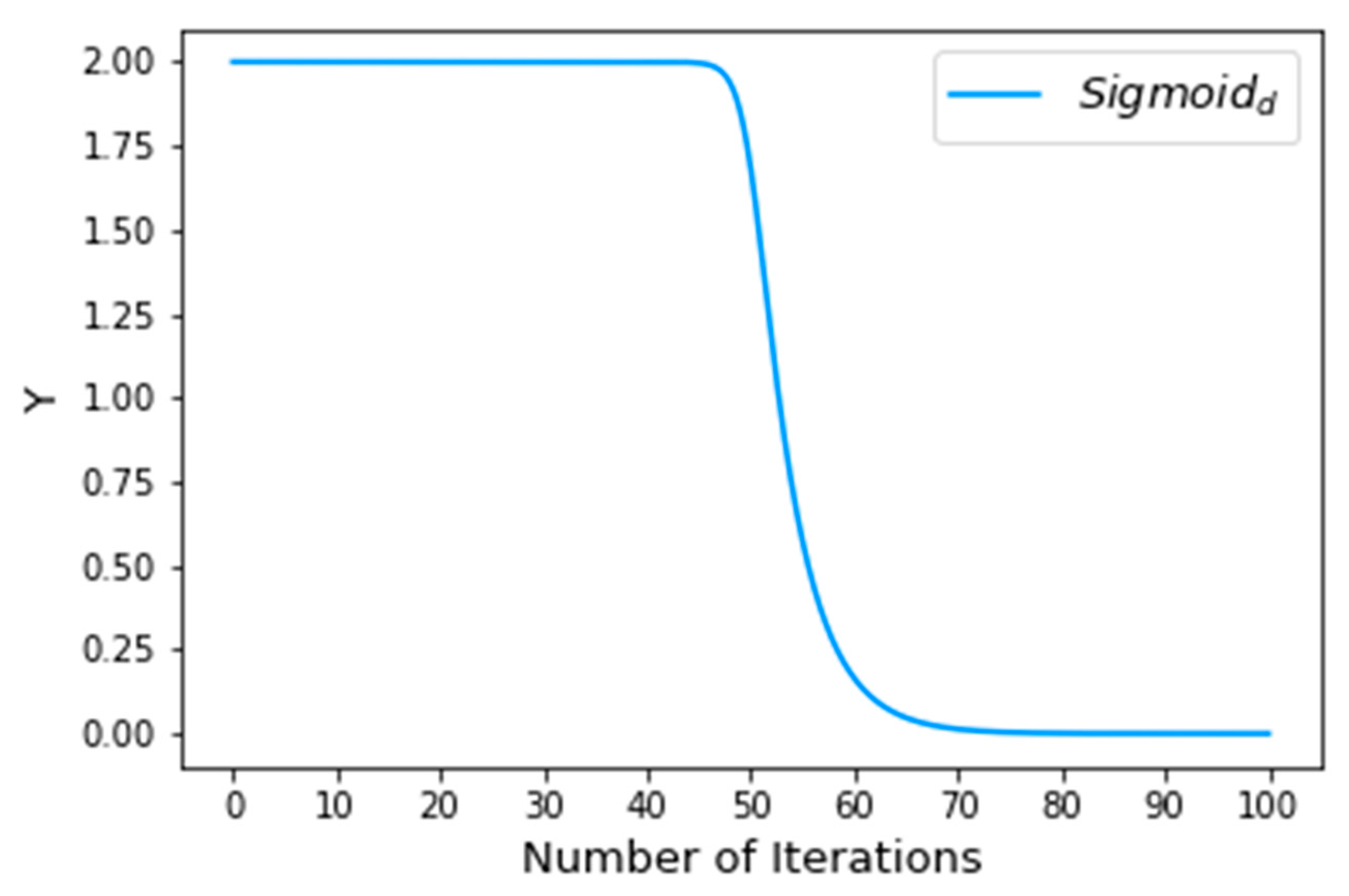
where is the step length and is the visual field of the artificial fish. Here, we used a deformed sigmoid function:
where is the current iteration number and is the maximum number of iterations. In this paper, we set = 100. The deformed sigmoid function is shown in Figure 2.
In the initial stages, the artificial fish’s field of view and step size are larger, which is conducive to speeding up the convergence and jumping out of a local optimum. The initial decay rate of the deformed sigmoid function is relatively slow, so the artificial fish has enough time to identify the optimal space with its larger field of view and can jump out of a local optimum to the global optimum with its larger step size. In the later stages, the field of view and step size are smaller, but the artificial fish has enough time for a refined search in the neighborhood of the global optimum to improve the accuracy of the solution found.
4.3. Adaptive Weight Factor
As can be seen from Section 4.2, the artificial fish can use a dynamic step size and field of view, which improves the convergence speed and optimization accuracy of the algorithm. However, when the artificial fish is moving from one local optimum, it may reach another local optimum beyond the global optimum because the dynamic step size cannot be adjusted according to the real-time artificial fish state. Alternatively, it may linger near the global optimum and converge to the global optimum only when the step size is small enough, which reduces the convergence speed. Thus, we propose an adaptive weight factor:
For an artificial fish with current state , it explores the next state where
When the artificial fish moves from state to state , if , then the current position of the artificial fish is far from the global optimum, so the step size needs to be as large as possible to accelerate the convergence. Moreover, if is close to , then the artificial fish is currently in a good neighborhood. Therefore, a smaller step size is better for refining the search to adjacent areas, which can improve the optimization accuracy of the algorithm.
4.4. Crossover and Mutation
Because AFSA may easily fall into a local optimum in the late stages, a crossover or mutation is applied. This approach gives it a stronger ability to jump out of a local optimum, thus improving the possibility of reaching the global optimum.
The prerequisites for performing crossover and mutation operations are as follows. Set a threshold . If the current optimum does not change after successive iterations, crossover and mutation operations will be carried out. Algorithm 2 is the specific step of crossover operation. Algorithm 3 is the specific step of mutation operation. Figure 3 is a schematic diagram of the crossover operation. Figure 4 is a schematic diagram of the mutation operation.
Crossover operation swaps components in one state with those in another state :
| Algorithm 2. Crossover operation |
| Input: the current population and . |
| Output: the new population . |
| Process: |
|
Mutation operation: This randomly changes a value in the state :
| Algorithm 3. Mutation operation |
| Input: the new population , and . |
| Output: the new population . |
| Process: |
|
4.5. Coding
Coding is used to map a problem into a model, as this can be more convenient and intuitive for finding a solution. In the design of AFSA, the selection of appropriate code directly affects the convergence speed and optimization accuracy of the algorithm.
At present, common coding methods include group coding, binary coding, and multi-value coding. For the STT scheduling problem in a secure cloud environment described in this paper, the group coding method can use multiple codes to represent the same allocation scheme, which is obviously not conducive for optimizing the search. In contrast, although the binary encoding method is unique, it is not conducive for visually displaying the allocation results. Moreover, suppose that the number of STTs is and the number of VSCRs is , then the search space for binary encoding is , while the search space for multi-value encoding is , which leads to a significantly better search efficiency. Moreover, the decoding of a multi-value encoding is simple, and the possibility of producing illegal solutions (a distribution scheme that is not unique) is eliminated when the artificial fish swims. Therefore, in this paper, we adopt multi-value coding for STT scheduling in a secure cloud environment.
Assume that the task-scheduling problem has m STTs and n VSCRs. It uses an assignment array, , where is the assignment . For example, indicates that the first STT is processed on the second VSCR, the second and fourth STTs are processed on the first VSCR, and the third STT is processed on the third VSCR.
4.6. Algorithm Process
A flowchart for MOOAFSA is shown in Figure 5. The main steps are in the Algorithm 4.
| Algorithm 4. MOOAFSA |
| Input: randomly generate a random vector of size , . |
| Output: the optimal scheduling scheme. |
| Process: |
|
5. Performance Validation
In this paper, we use the cloud simulator CloudSim [25], which is an extensible and universal simulation framework, to simulate the STT scheduling experiment.
5.1. Experimental Environment and Parameter Setting
The experiments were carried out with an Intel Xeon E5-2680 processor with 64 GB of memory running the Linux 64-bit operating system. The language used was Java.
During the experiment, we conducted the following two groups of experiments respectively, as shown in Table 5. Among them, the number of STTs started at 50 and was incremented by 50 until the maximum of 500 was reached.
To better simulate a real secure cloud platform, a reasonable and effective task-scheduling model was constructed. The ranges for the parameter values for the VSCRs and STTs are listed in Table 6. When creating VSCRs and STTs, the experimental parameters were randomly selected from the range but with uniform allocation in order to simulate computing resources with different levels of performance and STTs with different lengths.
In the experiments, different algorithms were compared. Because the algorithm parameters have a significant influence on the performance of the model, parameters common to more than one algorithm were set to the same value. At the same time, in order to ensure the fairness of the experiment, our experiment adopts the following methods: according to Refs. [26,27], we obtain the parameter recommended values of ant colony algorithm (ACO) and particle swarm optimization (PSO) algorithm, respectively. On this basis, we debug and optimize the algorithm parameters in combination with the simulation environment of this experiment and obtain the optimal value of the current algorithm as a comparative experiment. The specific parameters are shown in Table 7.
5.2. Experimental Results
To assess the performance of the STT scheduling strategy proposed in this paper, MOOAFSA was experimentally compared with ACO, PSO, and AFSA. The metrics used to evaluate the performance were the convergence speed, STT completion time, load balancing, and execution cost.
5.2.1. Rate of Convergence
The convergence of the algorithms was compared for 500 abnormal STTs and normal 500 STTs for 100 iterations. The experimental results are shown in Figure 6 and Figure 7.
As can be seen from the figures, compared with the other three algorithms, MOOAFSA converged fastest and had the highest convergence accuracy, for 500 abnormal STTs or 500 normal STTs. For ACO, the convergence rate was too slow in the early stages due to the low pheromone concentration. At the later stages, the accumulated pheromone concentration was too high, so it easily fell into a local optimum. For PSO, the initial convergence rate was fast. However, in the later stages, the loss of diversity in the search space led to a slow convergence rate and an inability to jump out of a local extreme value, resulting in premature convergence. AFSA had a fast convergence speed in the early stages, but in the later stages, due to the large step size and field of view, it could not converge to the optimal solution, resulting in oscillations and low optimization accuracy. MOOAFSA had the best convergence because chaotic tent mapping was used to initialize the artificial fish swarm, which effectively maintained the diversity of the population, inhibited the algorithm from falling into a local optimum, and improved the global search ability. Moreover, in MOOAFSA, the step size of the artificial fish were both optimized by using an adaptive weight factor. The algorithm dynamically adjusted the field of view and step size of the artificial fish during the iterations to accelerate the global convergence and improve the optimization accuracy. Finally, MOOAFSA applied crossovers and mutations to improve its ability to jump out of a local optimum.
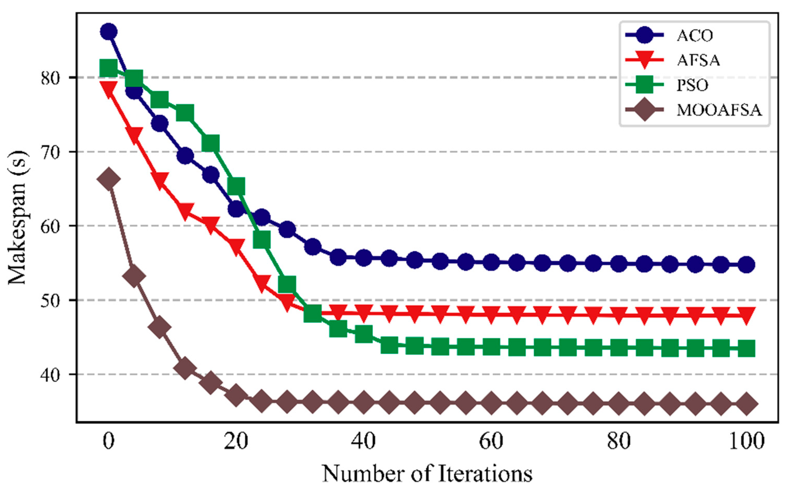
5.2.2. Completion Time
According to the experimental results shown in Figure 8 and Figure 9, we can see that MOOAFSA had an obviously lower completion time compared with the other three algorithms for different numbers of STTs. The completion times for ACO and PSO were initially very similar, but with an increase in the number of STTs, the completion times for ACO were significantly higher than for PSO. This is because the heuristic function of the ant colony algorithm is the reciprocal of the expected execution time of the STT on a virtual security resource. When the number of STTs to be scheduled was small, there were enough VSCRs and there was little resource competition among the STTs. As the number of STTs increased, ACO tended to allocate a large number of STTs to virtual security resource nodes with better performance, which made the overall completion time too long. Both PSO and AFSA tended to fall into a local optimum in the late stages, which increased the completion time. As the number of STTs increased, MOOAFSA had significantly lower completion times. Therefore, MOOAFSA performed best at scheduling a large number of STTs in a secure cloud.
As can be seen from Table 9, compared with ACO, AFSA, and PSO, the STT completion times (abnormal STTs) for MOOAFSA was reduced by an average of 15.62–28.69%, and the STT completion times (normal STTs) for MOOAFSA was reduced by an average of 10.84–17.44%. These results demonstrate the superiority of MOOAFSA in terms of completion time.
5.2.3. Load Balancing
As can be seen from Figure 10 and Figure 11, the load balancing performance of ACO, PSO, and AFSA gradually deteriorated with an increase in the number of STTs, whereas MOOAFSA balanced the load well. The metric for load balancing was lower for MOOAFSA than for the other three algorithms. With an increase in the number of STTs, for MOOAFSA, the metric for load balancing remained stable. This is because MOOAFSA quantified the load on different virtual security resources in a secure cloud environment and applied a dynamic load balancing strategy. MOOAFSA ensured that the load on the virtual secure resources was balanced, and this advantage became more obvious as the number of STTs increased.
As can be seen from Table 10, compared with ACO, AFSA, and PSO, the load balance degree (abnormal STTs) for MOOAFSA was reduced by an average of 66.91–75.62%, and the load balance degree (normal STTs) for MOOAFSA was reduced by an average of 74.26–78.58%. These results demonstrate the superiority of MOOAFSA in terms of load balance degree.
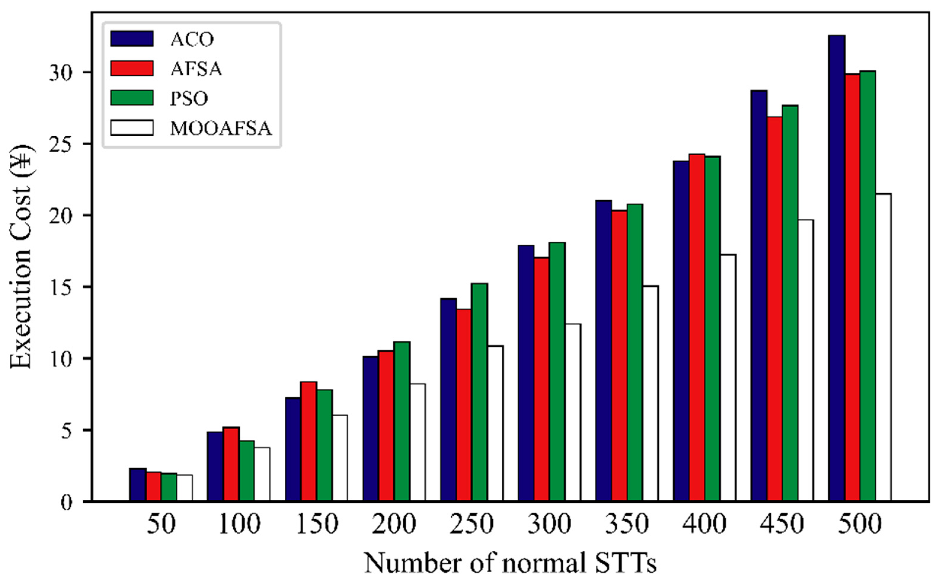
5.2.4. Execution Cost
Figure 12 and Figure 13 clearly shows that the overall execution costs for MOOAFSA were significantly lower than those for the other three algorithms. Further observation shows that as the number of STTs to be scheduled increased, the rate of increase of the execution costs for ACO, PSO, and AFSA was higher. This is because, for a large number of STTs, the competition for virtual security resources became intensified. ACO, PSO, and AFSA also consider the STT completion time when scheduling, so it was inevitable that some STTs were assigned to virtual security resource nodes with a relatively high execution cost, thus increasing the overall execution cost. In contrast, MOOAFSA considers the execution cost when scheduling STTs. Under the same conditions, MOOAFSA always tended to assign STTs to virtual secure resource nodes with a relatively low execution cost, which reduced the overall execution cost to some extent.
As can be seen from Table 11, compared with ACO, AFSA, and PSO, the execution cost (abnormal STTs) for MOOAFSA was reduced by an average of 32.3–41.31%, and the execution cost (normal STTs) for MOOAFSA was reduced by an average of 23.91–25.25%. These results demonstrate the superiority of MOOAFSA in terms of execution cost.
In conclusion, MOOAFSA performed better than ACO, AFSA, or PSO in terms of convergence speed, STT completion time, load balancing, and execution cost. Therefore, the STT scheduling strategy proposed in this paper is feasible.
6. Conclusions
In order to improve the STT scheduling of power business deployed on secure cloud, we build a secure cloud task-scheduling model that combined with the power information system. On this basis, we proposed MOOAFSA. MOOAFSA initializes the fish population through chaotic mapping, which improves the global optimization capability. Moreover, MOOAFSA uses a dynamic step size and field of view, as well as the introduction of adaptive weight factor, which accelerates the convergence and improves optimization accuracy. Finally, MOOAFSA applies crossovers and mutations, which make it easier to jump out of a local optimum. Our experimental results show that compared with ACO, PSO, and AFSA, the proposed algorithm had better convergence speed, STT completion time, load balancing, and execution cost. Moreover, as the number of the STTs increased, the advantages of MOOAFSA became more significant. Therefore, MOOAFSA is suitable for STT scheduling in a secure cloud environment.
In future work, we will study fault tolerance in a secure cloud environment and consider how to combine fault tolerance with the algorithm proposed in this paper to enhance the reliability of STT scheduling for a secure cloud.
Author Contributions
Conceptualization, W.L. and Q.F.; methodology, Q.F. and Y.J.; software, Q.F. and H.W.; validation, Q.F.; resources, Q.F. and H.W.; writing–original draft preparation, Q.F.; writing–review and editing, Q.F., F.D., S.L. and X.Z. All authors have read and agreed to the published version of the manuscript.
Funding
This work was financially supported by the science and technology project of State Grid Henan Electric Power Company: “Research and application of key technologies of adaptive protection for State Grid Cloud Security” (Grand No. SGHAXT00YJJS2100034).
Institutional Review Board Statement
Not applicable.
Informed Consent Statement
Not applicable.
Data Availability Statement
Not applicable.
Conflicts of Interest
The authors declare no conflict of interest.
References
- Luo, X.; Zhang, S.; Litvinov, E. Practical Design and Implementation of Cloud Computing for Power System Planning Studies. Smart Grid. IEEE Trans. Smart Grid 2018, 10, 2301–2311. [Google Scholar] [CrossRef]
- Anushree, B.; Arul Xavier, V.M. Comparative Analysis of Latest Task Scheduling Techniques in Cloud Computing environment. In Proceedings of the Second International Conference on Computing Methodologies and Communication (ICCMC 2018), Erode, India, 15–16 February 2018; pp. 608–611. [Google Scholar]
- Han, P.; Du, C.; Chen, J. A DEA Based Hybrid Algorithm for Bi-objective Task Scheduling in Cloud Computing. In Proceedings of the 5th IEEE International Conference on Cloud Computing and Intelligence Systems (CCIS 2018), Nanjing, China, 23–25 November 2018; pp. 63–67. [Google Scholar]
- Li, X.L.; Qian, J.X. Studies on artificial fish swarm optimization algorithm based on decomposition and coordination techniques. J. Circuits Syst. 2003, 1, 1–6. [Google Scholar]
- Qi, B.; Xiong, L.; Wang, L.; Chen, Z.; Huang, L. A Weights and Improved Adaptive Artificial Fish Swarm Algorithm for Path Planning. In Proceedings of the 2019 IEEE 8th Joint International Information Technology and Artificial Intelligence Conference (ITAIC), Chongqing, China, 24–26 May 2019; pp. 1698–1702. [Google Scholar]
- Xin-yue, L.; Kai-yao, Y.; Dong-min, X. The Research on the Coordinated Control System of PID Neural Network Based on Artificial Fish Swarm Algorithm. In Proceedings of the Chinese Control and Decision Conference (CCDC 2016), Yinchuan, China, 28–30 May 2016; pp. 3065–3068. [Google Scholar]
- Fu, M.; Fei, T.; Zhang, L.; Li, H. Research on Location Optimization of Low-Carbon Cold Chain Logistics Distribution Center by FWA-Artificial Fish Swarm Algorithm. In Proceedings of the International Conference on Communications, Information System and Computer Engineering (CISCE 2021), Beijing, China, 14–16 May 2021; pp. 529–533. [Google Scholar]
- Chiang, M.L.; Hsieh, H.C.; Tsai, W.C.; Ke, M.C. An improved task scheduling and load balancing algorithm under the heterogeneous cloud computing network. In Proceedings of the 2017 IEEE 8th International Conference on Awareness Science and Technology (iCAST), Taichung, Taiwan, 8–10 November 2017; pp. 290–295. [Google Scholar]
- Panda, S.K.; Jana, P.K. SLA-based task scheduling algorithms for heterogeneous multi-cloud environment. J. Supercomput. 2017, 73, 2730–2762. [Google Scholar] [CrossRef]
- Mao, H.; Schwarzkopf, M.; Venkatakrishnan, S.B.; Meng, Z.; Alizadeh, M. Learning Scheduling Algorithms for Data Processing Clusters. In Proceedings of the ACM Special Interest Group on Data Communication, Beijing, China, 19–23 August 2019; pp. 270–288. [Google Scholar]
- Adhikari, M.; Nandy, S.; Amgoth, T. Meta heuristic-based task deployment mechanism for load balancing in IaaS cloud. J. Netw. Comput. Appl. 2019, 128, 64–77. [Google Scholar] [CrossRef]
- Narayanan, D.; Santhanam, K.; Kazhamiaka, F.; Phanishayee, A.; Zaharia, M. Heterogeneity-Aware Cluster Scheduling Policies for Deep Learning Workloads. In Proceedings of the 14th USENIX Symposium on Operating Systems Design and Implementation, Banff, AB, Canada, 4–6 November 2020; pp. 481–498. [Google Scholar]
- Ding, D.; Fan, X.; Zhao, Y.; Kang, K.; Yin, Q.; Zeng, J. Q-learning based dynamic task scheduling for energy-efficient cloud computing. Future Gener. Comput. Syst. 2020, 108, 361–371. [Google Scholar] [CrossRef]
- Devaraj, A.F.S.; Elhoseny, M.; Dhanasekaran, S.; Lydia, E.L.; Shankar, K. Hybridization of firefly and Improved Multi-Objective Particle Swarm Optimization algorithm for energy efficient load balancing in Cloud Computing environments. J. Parallel Distrib. Comput. 2020, 142, 36–45. [Google Scholar] [CrossRef]
- Li, J.Q.; Han, Y.Q. A hybrid multi-objective artificial bee colony algorithm for flexible task scheduling problems in cloud computing system. Clust. Comput. 2020, 23, 2483–2499. [Google Scholar] [CrossRef]
- Domanal, S.G.; Guddeti, R.M.R.; Buyya, R. A hybrid bio-inspired algorithm for scheduling and resource management in cloud environment. IEEE Trans. Serv. Comput. 2020, 13, 3–15. [Google Scholar] [CrossRef]
- Mondal, S.S.; Sheoran, N.; Mitra, S. Scheduling of time-varying workloads using reinforcement learning. In AAAI Conference on Artificial Intelligence; AAAI Press: Palo Alto, CA, USA, 2021; Volume 35, pp. 9000–9008. [Google Scholar]
- Teylo, L.; Arantes, L.; Sens, P.; Drummond, L. A dynamic task scheduler tolerant to multiple hibernations in cloud environments. Clust. Comput. 2021, 24, 1051–1073. [Google Scholar] [CrossRef]
- Abualigah, L.; Diabat, A. A novel hybrid antlion optimization algorithm for multi-objective task scheduling problems in cloud computing environments. Clust. Comput. 2021, 24, 205–223. [Google Scholar] [CrossRef]
- Shelke, M.P.K.; Sontakke, M.S.; Gawande, A.D. Intrusion detection system for cloud computing. Int. J. Sci. Technol. Res. 2012, 1, 67–71. [Google Scholar]
- Casola, V.; De Benedictis, A.; Rak, M.; Villano, U. Towards automated penetration testing for cloud applications. In Proceedings of the 2018 IEEE 27th International Conference on Enabling Technologies: Infrastructure for Collaborative Enterprises (WETICE), Paris, France, 27–29 June 2018; pp. 24–29. [Google Scholar]
- Lingkang, Z.; Yuwei, L.; Xue, J. Detection of Abnormal Data Flow at Network Boundary of Renewable Energy Power System. In Proceedings of the 2020 IEEE 3rd International Conference on Automation, Electronics and Electrical Engineering (AUTEEE), Shenyang, China, 20–22 November 2020; pp. 309–312. [Google Scholar]
- Gao, Z.; Zhao, J.; Li, S.; Hu, R. The Improved Equilibrium Optimization Algorithm with Tent Map. In Proceedings of the 5th International Conference on Computer and Communication Systems (ICCCS 2020), Shanghai, China, 15–18 May 2020; pp. 343–346. [Google Scholar]
- Gao, Z.; Zhao, J.; Hu, Y.; Chen, H. The Improved Harris Hawk Optimization Algorithm with the Tent Map. In Proceedings of the 3rd International Conference on Electronic Information Technology and Computer Engineering (EITCE 2019), Xiamen, China, 18–20 October 2019; pp. 336–339. [Google Scholar]
- Rani, E.; Kaur, H. Study on fundamental usage of CloudSim simulator and algorithms of resource allocation in cloud computing. In Proceedings of the 2017 8th International Conference on Computing, Communication and Networking Technologies (ICCCNT), Delhi, India, 3–5 July 2017; pp. 1–7. [Google Scholar]
- Duan, H.; Ma, G.; Liu, S. Experimental study of the adjustable parameters in basic ant colony optimization algorithm. In Proceedings of the 2007 IEEE Congress on Evolutionary Computation, Singapore, 25–28 September 2007; pp. 149–156. [Google Scholar]
- Jiang, M.; Luo, Y.P.; Yang, S.Y. Stochastic convergence analysis and parameter selection of the standard particle swarm optimization algorithm. Inf. Process. Lett. 2007, 102, 8–16. [Google Scholar] [CrossRef]
- Wu, C.; Toosi, A.N.; Buyya, R.; Ramamohanarao, K. Hedonic Pricing of Cloud Computing Services. IEEE Trans. Cloud Comput. 2021, 9, 182–196. [Google Scholar] [CrossRef] [Green Version]
- Kandpal, M.; Patel, K. Pricing Model for Revenue Generation using Recurrent Neural Network for Cloud Service Provider. In Proceedings of the 3rd International Conference on Trends in Electronics and Informatics (ICOEI 2019), Tirunelveli, India, 23–25 April 2019; pp. 988–992. [Google Scholar]
Figure 1.
STT scheduling model for a secure cloud.

Figure 2.
Deformed sigmoid function ( = 100).

Figure 3.
Crossover operation.

Figure 4.
Mutation operation.

Figure 5.
Flow chart for MOOAFSA.

Figure 6.
Comparison of convergence (number of abnormal STTs was 500).

Figure 7.
Comparison of convergence (number of normal STTs was 500).

Figure 8.
Comparison of STT completion times for different numbers of abnormal STTs.

Figure 9.
Comparison of STT completion times for different numbers of normal STTs.

Figure 10.
Comparison of load balancing for different numbers of abnormal STTs.

Figure 11.
Comparison of load balancing for different numbers of normal STTs.

Figure 12.
Comparison of execution cost for different numbers of abnormal STTs.

Figure 13.
Comparison of execution cost for different numbers of normal STTs.


Table 1.
Related works regarding task scheduling.
| Reference | Year | Algorithm | Indicator | Advantage |
|---|---|---|---|---|
| [8] | 2017 | AMS | Makespan Load balancing | AWS can obtain good task completion time and achieve load balancing in cloud computing network. |
| [9] | 2017 | SLA-MCT SLA-Min-Min | Makespan Resource Utilization Cost | The proposed algorithm achieves a proper balance between manufacturing time and service gain cost. |
| [10] | 2019 | Decima | Makespan | Decima can help improve resource utilization by automatically learning highly efficient, workload-specific scheduling policies. Decima’s policies are particularly effective during periods of high cluster load. |
| [11] | 2019 | LB-RC | Makespan Execution cost Load balancing | LB-RC algorithm can reduce the execution time and completion time of tasks while meeting deadlines, and maintain the load balance of resources. |
| [12] | 2020 | Gavel | Makespan Throughput Average job completion time Fairness | Gavel uses a decoupled round-based scheduling mechanism to ensure that the computed optimal allocation is realized. Gavel’s heterogeneity-aware policies improve end objectives both on a physical and simulated cluster. |
| [13] | 2020 | QEEC | Average response time Energy consumption | Maximizing the service capability of each virtual machine can effectively reduce the energy consumption in the cloud environment. |
| [14] | 2020 | FIMPSO | Makespan Load balancing Throughput Resource Utilization | FIMPSO achieved effective average load for making and enhanced the essential measures like proper resource usage and response time of the tasks. |
| [15] | 2020 | LABC | Makespan Fitness value Average calculation time | LABC algorithm has strong development ability and local search ability. |
| [16] | 2020 | HYBRID Bio-Inspired | Makespan Load balancing Response time Resource Utilization | HYBRID Bio-Inspired algorithm realizes resource load balancing, reduces execution time and improves resource utilization. |
| [17] | 2021 | TVW-RL | Resource Utilization Resource Fragmentation Resource Overshoot | TVW-RL improves resource utilization, reduces resource fragments and the number of machines used. |
| [18] | 2021 | HADS | Monetary costs | HADS can minimize the monetary costs of bag-of-tasks, respecting the application’s deadline and avoiding temporal failures. |
| [19] | 2021 | MALO | Makespan Load balancing Response time | For large search space, MALO has faster convergence speed and is suitable for large-scale scheduling problems. |
Table 2.
Description of acronyms used in the proposed model definition.
| Symbol | Description | Symbol | Description |
|---|---|---|---|
| The length of the STT | The size of the STT before execution | ||
| The size of the STT after execution | The type of the STT | ||
| The risk level of the STT | The computing capacity of the VSCR | ||
| The bandwidth of the VSCR | The running memory of the VSCR | ||
| The number of CPUs of the VSCR | The storage size of the VSCR | ||
| Time consumed by VSCR to execute STT | Assignment relation between STT and VSCR | ||
| Transfer time of STT on VSCR | Time consumed by VSCR to complete STT | ||
| Unit computation cost | Unit bandwidth cost | ||
| Unit memory cost | Unit storage cost | ||
| Performance of VSCR | Load on VSCR | ||
| Average load on all VSCRs | System load evaluation metrics | ||
| The category of the VSCR |
Table 3.
Attack type of abnormal STTs.
| Type | Harm |
|---|---|
| Traditional network attacks [22] | For example, distributed denial of service attack (DDoS). It can make use of some defects of network protocol and operating system to carry out network attack, fill the server with a large number of information to be replied, consume network bandwidth or system resources, and cause the network or system to be overloaded and paralyzed to stop providing normal network services. |
| Invisible penetration and scanning [22] | This kind of attack means that the attacker initiates an intrusion from outside the target network in order to steal or destroy important assets in the target network. During this period, the attacker continues to use several vulnerabilities in the target network to invade and finally complete a series of attacks on the target. |
| Hide disguised communications [22] | It is a kind of antagonism network attack, using the hidden means of invasion, and its network communication is disguised as or concealed in the normal legal network data flow to avoid terminal level and network level of safety inspection in order to reside for a long time and can control the victim host or device, achieve the goal of continuing to steal information or long-term control using. |
| Attack aimed at application layer vulnerabilities [22] | Hackers send disguised data requests to users for loopholes in the application layer so as to achieve the purpose of illegal data theft, illegal data tampering, system paralysis and other attacks. |
Table 4.
Main parameter characteristics of AFSA.
| Parameter | Value | Advantages | Disadvantages |
|---|---|---|---|
| Step size | Too high | There are fewer iterations and convergence is faster. | Optimization accuracy is not high, and oscillations can occur outside a certain range (the number of iterations increases, and the convergence is slower). |
| Too low | Optimization accuracy is improved. | There are more iterations, convergence is slow, and it may easily fall into a local optimum. | |
| Field of view | Too wide | Global search capability is enhanced and the convergence is faster. | Optimization accuracy is low. |
| Too narrow | Local search ability is enhanced and optimization accuracy is improved. | Convergence is slow. |
Table 5.
Experimental environment.
| Experiment | Object | Number |
|---|---|---|
| Experiment 1 | VSCR | 15 |
| Abnormal STTs | 50–500 | |
| Experiment 2 | VSCR | 15 |
| Normal STTs | 50–500 |
Table 6.
Parameters for the secure cloud model.
| Object | Parameter | Value |
|---|---|---|
| VSCR | Processing speed (MIPS): | 200–500 |
| Bandwidth (Mb/s): | 50–200 | |
| Memory (GB): | 2–16 | |
| Number of CPU cores: | 2–8 | |
| Storage capacity (GB): | 50–200 | |
| Category: | 1–8 | |
| STT | Length of the STT (MI): | 2000–6000 |
| Pre-execution size (MB): | 200–300 | |
| Post-execution size (MB): | 200–300 | |
| Category: | 1–8 | |
| Risk level: | 1–4 |
Table 7.
Parameters for the algorithms.
| Algorithm | Parameter | Value |
|---|---|---|
| AFSA, MOOAFSA | Number of attempts: | 3 |
| Step length: | 2.5 | |
| Field of vision: | 3.5 | |
| Crowding factor: | 2 | |
| Threshold: | 5 | |
| MOOAFSA | Computing power weight: | 0.75 |
| Bandwidth size weight: | 0.25 | |
| ACO | Information heuristic factor: | 2.5 |
| Expectation heuristic factor: | 5.5 | |
| Information volatile factor: | 0.35 | |
| Pheromone increment: | 100 | |
| PSO | Learning factor 1: | 1.5 |
| Learning factor 2: | 2 | |
| Inertial factor: | 0.9 | |
| ACO, PSO, AFSA, MOOAFSA | Number of iterations: | 100 |
| Population size: | 40 |
Table 8.
Unit prices for the VSCR.
| Resource Type | Unit Pricing | Unit Price |
|---|---|---|
| CPU | CNY per core per hour | 0.46 |
| RAM | CNY per GB per hour | 0.04 |
| Bandwidth | CNY per Mbps per hour | 0.03 |
| Disk | CNY per GB per hour | 0.008 |
Table 9.
Comparison of STT completion times for different numbers of STTs.
| Number of VSCRs | Number of STTs | STT Completion Time (s) | |||||||
|---|---|---|---|---|---|---|---|---|---|
| Abnormal | Normal | ||||||||
| ACO | AFSA | PSO | MOOAFSA | ACO | AFSA | PSO | MOOAFSA | ||
| 15 | 50 | 47.84 | 41.01 | 42.37 | 26.72 | 5.36 | 5.12 | 5.24 | 5.06 |
| 100 | 89.63 | 71.32 | 80.91 | 50.83 | 10.68 | 9.30 | 9.63 | 9.18 | |
| 150 | 127.46 | 101.58 | 123.12 | 90.12 | 16.98 | 17.63 | 16.42 | 13.25 | |
| 200 | 142.50 | 139.55 | 151.01 | 128.38 | 20.35 | 19.14 | 19.87 | 17.09 | |
| 250 | 204.43 | 176.66 | 191.31 | 156.27 | 23.97 | 23.01 | 24.58 | 21.32 | |
| 300 | 245.75 | 219.78 | 234.43 | 187.49 | 29.83 | 26.32 | 28.87 | 25.27 | |
| 350 | 279.37 | 241.89 | 276.53 | 210.12 | 34.29 | 30.41 | 33.12 | 27.89 | |
| 400 | 366.94 | 288.26 | 314.57 | 255.48 | 37.61 | 34.59 | 35.97 | 30.21 | |
| 450 | 389.96 | 310.25 | 354.69 | 283.37 | 40.16 | 38.09 | 39.05 | 32.99 | |
| 500 | 426.24 | 344.31 | 394.48 | 296.22 | 54.78 | 47.89 | 43.52 | 36.04 | |
Table 10.
Comparison of load balancing for different numbers of STTs.
| Number of VSCRs | Number of STTs | Load Balance Degree | |||||||
|---|---|---|---|---|---|---|---|---|---|
| Abnormal | Normal | ||||||||
| ACO | AFSA | PSO | MOOAFSA | ACO | AFSA | PSO | MOOAFSA | ||
| 15 | 50 | 3.12 | 3.53 | 4.51 | 1.04 | 2.73 | 2.97 | 3.15 | 0.81 |
| 100 | 3.65 | 3.31 | 4.48 | 1.95 | 3.06 | 3.16 | 3.46 | 0.94 | |
| 150 | 4.24 | 3.62 | 5.17 | 1.72 | 3.57 | 3.32 | 3.89 | 1.16 | |
| 200 | 5.31 | 3.98 | 5.83 | 1.84 | 3.85 | 3.51 | 4.25 | 1.07 | |
| 250 | 5.88 | 4.11 | 5.92 | 1.73 | 4.03 | 3.67 | 4.61 | 1.01 | |
| 300 | 6.67 | 4.56 | 5.98 | 1.32 | 4.19 | 3.82 | 4.79 | 0.93 | |
| 350 | 7.49 | 5.23 | 6.89 | 1.23 | 4.52 | 4.01 | 5.01 | 0.97 | |
| 400 | 8.02 | 5.99 | 7.53 | 1.30 | 4.89 | 4.17 | 5.37 | 0.91 | |
| 450 | 8.87 | 6.83 | 8.60 | 1.21 | 5.17 | 4.33 | 5.72 | 0.85 | |
| 500 | 10.26 | 7.95 | 9.89 | 1.18 | 5.88 | 4.77 | 6.01 | 0.83 | |
Table 11.
Comparison of execution cost for different numbers of STTs.
| Number of VSCRs | Number of STTs | Execution Cost (¥) | |||||||
|---|---|---|---|---|---|---|---|---|---|
| Abnormal | Normal | ||||||||
| ACO | AFSA | PSO | MOOAFSA | ACO | AFSA | PSO | MOOAFSA | ||
| 15 | 50 | 24.01 | 18.96 | 16.98 | 11.10 | 2.31 | 2.05 | 1.96 | 1.85 |
| 100 | 36.12 | 38.04 | 33.02 | 17.01 | 4.87 | 5.19 | 4.26 | 3.78 | |
| 150 | 76.22 | 61.42 | 67.21 | 34.13 | 7.23 | 8.36 | 7.81 | 6.03 | |
| 200 | 85.88 | 78.12 | 87.16 | 49.79 | 10.12 | 10.51 | 11.16 | 8.24 | |
| 250 | 122.14 | 98.93 | 110.20 | 60.32 | 14.15 | 13.44 | 15.23 | 10.87 | |
| 300 | 150.67 | 113.42 | 131.12 | 89.27 | 17.88 | 17.03 | 18.09 | 12.42 | |
| 350 | 178.20 | 148.96 | 157.63 | 114.56 | 21.02 | 20.31 | 20.76 | 15.06 | |
| 400 | 219.21 | 200.16 | 239.64 | 168.23 | 23.78 | 24.26 | 24.09 | 17.24 | |
| 450 | 282.42 | 264.33 | 273.15 | 203.17 | 28.67 | 26.87 | 27.64 | 19.66 | |
| 500 | 344.25 | 312.56 | 325.47 | 238.17 | 32.54 | 29.84 | 30.06 | 21.48 | |
Publisher’s Note: MDPI stays neutral with regard to jurisdictional claims in published maps and institutional affiliations. |
© 2022 by the authors. Licensee MDPI, Basel, Switzerland. This article is an open access article distributed under the terms and conditions of the Creative Commons Attribution (CC BY) license (https://creativecommons.org/licenses/by/4.0/).
Share and Cite
MDPI and ACS Style
Li, W.; Fan, Q.; Dang, F.; Jiang, Y.; Wang, H.; Li, S.; Zhang, X. Multi-Objective Optimization of a Task-Scheduling Algorithm for a Secure Cloud. Information 2022, 13, 92. https://0-doi-org.brum.beds.ac.uk/10.3390/info13020092
AMA Style
Li W, Fan Q, Dang F, Jiang Y, Wang H, Li S, Zhang X. Multi-Objective Optimization of a Task-Scheduling Algorithm for a Secure Cloud. Information. 2022; 13(2):92. https://0-doi-org.brum.beds.ac.uk/10.3390/info13020092
Chicago/Turabian StyleLi, Wei, Qi Fan, Fangfang Dang, Yuan Jiang, Haomin Wang, Shuai Li, and Xiaoliang Zhang. 2022. "Multi-Objective Optimization of a Task-Scheduling Algorithm for a Secure Cloud" Information 13, no. 2: 92. https://0-doi-org.brum.beds.ac.uk/10.3390/info13020092
Note that from the first issue of 2016, this journal uses article numbers instead of page numbers. See further details here.