
Editing Compression Dictionaries toward Refined Compression-Based Feature-Space

Department of Computer and Network Engineering, University of Electro-Communications, Tokyo 182-8585, Japan
*
Author to whom correspondence should be addressed.
Information 2022, 13(6), 301; https://0-doi-org.brum.beds.ac.uk/10.3390/info13060301
Submission received: 14 April 2022
/
Revised: 5 June 2022
/
Accepted: 10 June 2022
/
Published: 15 June 2022
(This article belongs to the Section Information Theory and Methodology)
Abstract
:This paper investigates how to construct a feature space for compression-based pattern recognition which judges the similarity between two objects x and y through the compression ratio to compress x with y (’s dictionary). Specifically, we focus on the known framework called PRDC, which represents an object x as a compression-ratio vector (CV) that lines up the compression ratios after x is compressed with multiple different dictionaries. By representing an object x as a CV, PRDC makes it possible to apply vector-based pattern recognition techniques to the compression-based pattern recognition. For PRDC, the dimensions, i.e., the dictionaries determine the quality of the CV space. This paper presents a practical technique to modify the chosen dictionaries in order to improve the performance of pattern recognition substantially: First, in order to make the dictionaries independent from each other, our method leaves any word shared by multiple dictionaries in only one dictionary and assures that any pair of dictionaries have no common words. Next, we transfer words among the dictionaries, so that all the dictionaries may keep roughly the same number of words and acquire the descriptive power evenly. The application to real image classification shows that our method increases classification accuracy by up to 8% compared with the case without our method, which demonstrates that our approach to keep the dictionaries independent is effective.
1. Introduction
With the prevalence of various new types of multimedia data in the big-data era, universal techniques to examine their characteristics at low cost without human intervention have been demanded more. Typical statistical pattern recognition involves the statistical modeling of data which accompanies the complicated configuration of parameters. Therefore, it does not necessarily meet this demand. Deep learning requires many training data and takes a long training time. Thus, it also does not satisfy the above demand.
By contrast, compression-based pattern recognition is a basically parameter-free approach toward automatic data analysis and can deal with any data types such as music, genome, and images universally at low cost, once they can be represented as strings. In principle, this approach measures the similarity between two objects x and y with the compression ratio to compress x with y (’s dictionary). NCD (Normalized Compression Distance) [1] is the most well-known representative of this technique and calculates the distance between two objects. Thus, NCD is fit for pattern recognition techniques based on the distance matrix such as spectral clustering [2] and agglomerative hierarchical clustering. In fact, it is quite common in compression-based pattern recognition to illustrate the clustering result as the Quartet tree [3] derived from the distance matrix. However, pattern recognition techniques based on the distance matrix often suffer from the inherent huge time complexity of , where n equals the number of data points. Moreover, application of NCD to vector-based techniques such as the k-means clustering and the SVM (Support Vector Machine) [4] classification is not immediate. Although the kernel trick can combine the SVM with NCD without representing objects as vectors [5], it will not generate general-purpose feature vectors that may be applied to any vector-based machine learning algorithms.
By contrast, Watanabe et al. developed a framework called PRDC (Pattern Representation on Data Compression) [6] in order to make use of the vector-based pattern recognition techniques, where an object x is expressed as an N-dimensional compression-ratio vector (CV) that lists the compression ratios to compress x with various N dictionaries. The performance of PRDC is strongly influenced by the N dictionaries spanning the compression vector space (CV space hereafter).
This paper proposes to modify the CV space for PRDC in order to enhance its quality. First, we edit the N base dictionaries and guarantee that any pair of dictionaries have no common words in order to make them independent from each other. Then, we reassign the remaining words to the N base dictionaries, so that each base dictionary may consist of roughly the same number of words. Our word reassignment still preserves the condition that any two base dictionaries share no common words. Specifically, we develop two types of word reassignment algorithms. The first algorithm REVIVAL does not change the original N base dictionaries radically. Thus, the i-th final base dictionary consists of a subset of the words held by the i-th original base dictionary. By contrast, the second algorithm VOCAB actively gathers words from multiple original base dictionaries and packs them into a single identical dictionary. The application to real image classification shows that both of our two methods improve pattern recognition accuracy as compared with the case without them.
This paper is organized as follows: Section 2 briefly reviews the related works on compression-based pattern recognition. Section 3 presents our new method to edit the dictionaries spanning the CV space. Section 4 describes the experimental evaluation and the discussion. Section 5 concludes this paper.
We remark here that this paper expands the contents of our international conference paper [7].
2. Literature Review: Compression-Based Pattern Recognition
This section summarizes the related works on compression-based pattern recognition. The compression-based pattern recognition has the advantage that it can be applied to general-purpose data such as Twitter data [8], music [9], image analysis [10,11], malware detection [12], and bioinformatics [13]. Throughout this section, we assume that objects are represented as one-dimensional strings.
2.1. Compression Distance
Originally, compression-based pattern recognition proposes to measure the dissimilarity between two objects without examining their minute structures. Let x and y be two objects. For instance, NCD computes the distance between x and y as in Equation (1)
where represents the size of the compressed version of x, and signifies the size of the file obtained by compressing the concatenation of x and y. The more common substrings x and y share, the smaller NCD () becomes because we can compress more compactly. According to [14], NCD implicitly maps x and y to a very high-dimensional compression feature space, where the number of dimensions equals the number of words in the compression dictionary. However, NCD does not produce feature vectors for x and y after all.
NDD (Normalized Dictionary Distance) [15] and FCD [16] (Fast Compression Distance) pay attention to the dictionaries yielded by the compressors like LZW (Lempel–Ziv–Welch) [17]. Different from NCD, both of them calculate the distance without the overhead incurred in data compression because they compare the dictionaries of x and y directly without compressing x with y (’s dictionary). Here, the dictionary of x consists of x’s substrings called words discovered when the compressor scans x. NMD [18,19] (Normalized Multiset Distance) counts how often the words in the dictionary appear in the object and exploits this information for the distance computation.
Recently, Field et al. [20] detected the boundaries in a data stream by measuring the SLID (Sliding Information Distance) between two adjacent sections, where the SLID measures the dissimilarity between the compression dictionaries extracted from the two sections.
2.2. PRDC
PRDC represents an object as an N-dimensional compression-ratio vector (CV). First, PRDC somehow decides a set of N base dictionaries , each of which is responsible for one dimension at the CV space. Then, the CV for an object x denoted by is defined as
Here, indicates the length of x, while presents the size of x after compressed by . Therefore, becomes the compression ratio of x via . Now that x is mapped to , we can make use of any vector-based pattern recognition technique such as SVM. PRDC relies on the LZW data compressor to derive dictionaries from strings.
For PRDC, the choice of N base dictionaries decides the performance of pattern recognition. As is desired for any feature space, each dimension should exhibit different properties. In [6], the developers of PRDC choose the base dictionaries as follows. Suppose that we have M objects, i.e., M strings at hand. They first construct an L-dimensional temporal CV space S by picking up L objects from T uniformly at random and by creating L temporal dictionaries from these L objects. Then, every object x in T is converted to the temporal CV referred to as in S. Next, after clustering the temporal CVs into N clusters in S, N representative objects are selected in such a way that a single representative object is chosen per cluster. As for the clustering in S, they implemented the k-means method [6,21]. Finally, these N objects provide the N base dictionaries which define the final CV space . In this way, PRDC expects to collect dictionaries of independent characteristics by selecting them from separated clusters. However, we consider that this idea does not always produce a good final CV space . Note that the axes in the temporal CV space S may be correlated, as they are chosen simply at random. When this phenomenon occurs, the clustering is performed on the shrunk S which actually has less than L dimensions, and will be damaged and cannot realize adequate pattern recognition. As a comprehensive metaphor, think of the clustering of pixel colors in one image. If we cluster the colors on the shrunk two-dimensional color space composed of “Red” and “Green” only, the representative colors will not realize effective color quantization.
From now on, we describe previous works other than PRDC that also construct a feature space by making use of data compression. Whereas PRDC [6] seeks the base dictionaries in an unsupervised way, Cilibrasi [22] chose them in a supervised way by selecting the equal number of representative objects evenly from all the object classes. That is, if one wants to obtain an N-dimensional CV space to address the classification problem involving C classes, objects are chosen per class. We refer to this method as “SUPERVISED” hereafter.
Ting et al. [23] utilized a compression distance vector for an object x, which lists the NCDs between x and multiple reference objects. Since they adopt all available objects as reference objects, the number of dimensions in grows as large as the total number of objects. To reduce the number of dimensions, [24] selects a moderate number of anchors (that is representative objects) from all of the objects. In the same way as PRDC, the compression distance vector spans a feature space based on data compression. However, it usually takes a longer time to generate than to generate because NCD must create the compression dictionary online while compressing objects.
Coltuc [25] et al. proposed another compression distance vector to represent an image x. In the compression distance vector for x, one coordinate value presents an NCD between x and an image which transforms x with simple geometric transforms such as circular shift and rotation. Unlike PRDC, their work assumes a specific pattern recognition task whose purpose is to recognize images which modify x with filtering, histogram equalization, and so on.
Finally, we refer to some previous works which correct the compression dictionaries. In order to speed up pattern classification, Ting et al. [26] defined the mean dictionary for multiple dictionaries, each of which originates from a training sample of the same class. They introduced a fast greedy algorithm to approximate the mean dictionary. Similarly, Contreras et al. [27] create a large dictionary per class by concatenating multiple dictionaries extracted from the training samples of the same class. It is true that these two methods construct a new dictionary by editing several known dictionaries. However, their goal is not to establish a good CV space, but to refine the k-NN classifier founded upon some compression distance.
3. Methods
Our research purpose is to construct a proper N-dimensional CV space. We consider this problem under a restriction that, to generate one N-dimensional CV, the data compression can be executed at most N times. Without this restriction, it is possible to compute a very high-dimensional compression vector by using a lot of dictionaries and to reduce the vector dimension to N with a PCA (Principal Component Analysis [28])-like technique. However, this approach spends too much time to compute an N-dimensional CV, as the heavy data compression operation must be iterated many times. Hence, this approach is not tolerable.
The core of compression-based pattern recognition has been to compute object-based dissimilarity measures like NCD. PRDC and SUPERVISED, which utilize the CV space, have also adopted this convention, such that one coordinate value of the CV for an object o represents the similarity value (that is, the compression ratio) between o and the real object associated with the axis of coordinates. The compression distance vector [23,24] also follows the convention. Our main contribution is to quit this convention so as to make a more useful CV space for pattern recognition. In particular, given a set of base dictionaries acquired by some dictionary selection algorithm such as PRDC and SUPERVISED, we devise a technique to edit them. As the result, in our scheme, one coordinate value of a CV does not represent the similarity value between a certain pair of real objects anymore.
Figure 1 illustrates how we modify the given N base dictionaries , where . Assume that these N base dictionaries have been chosen by some dictionary selection algorithm such as PRDC and SUPERVISED. First, to make the base dictionaries in D independent from each other, our method modifies them, so that no two dictionaries may have any common words. Section 3.1 will describe this process in detail. As described later, since this process prioritizes dictionaries with smaller subscripts, shall hold more words than if after the common words are deleted. Therefore, in the next step, we further modify the assignment of words to dictionaries, so that all of the dictionaries may consist of roughly the same number of words in order to enhance the expressive power of each dimension. This function will be explained in Section 3.2. We develop two kinds of word reassignment algorithms, that is, REVIVAL and VOCAB.
3.1. Removal of Common Words
Let be the N base dictionaries chosen by some dictionary selection algorithm to build an N-dimensional CV space. Usually, at this point, each member of D is generated by the data compression algorithm compressing some real object, and the dictionary selection algorithm tries to keep the dimensions of CV space independent from each other by choosing N objects of different features.
However, this strategy does not necessarily render the dimensions independent in practice. No matter how different the chosen objects are at the object level, the corresponding dictionaries can be correlated at the word level, as they share common words. That is, many words in are also likely to be contained in other dictionaries in D.
We mitigate this problem by editing the dictionaries, so that the dictionaries may become dissimilar at the word level. Our method modifies the dictionaries from to incrementally one by one. That is, it modifies (for ) after the i dictionaries from to are amended. Let and denote the set of words in before and after the modification, respectively. We examine every word w in and delete w, if w has already appeared in . Therefore, Equation (3) holds. Since for has already been modified before is processed, not but appears on the right-hand side of (3):
After all the base dictionaries are modified, it is guaranteed that any two different dictionaries in D never have any common words. Namely, for any satisfying , , . This proposition can be easily proved by induction. In this way, our modification algorithm raises the independence among the N base dictionaries at the word level.
Because the above algorithm behaves sensitively to the order of dictionaries, we sort the N dictionaries in advance. Here, we arrange the dictionaries in descending order of uniqueness in order to give higher priority to more unique dictionaries. We measure the uniqueness of a dictionary d by counting the number of words in d that are also included in the other dictionaries in D. This quantity is symbolized as and defined in Equation (4). We regard d as more unique, as becomes smaller:
After all, the dictionaries are sorted in the increasing order of . Thus, the most unique dictionary that has the least words common to the other dictionaries becomes .
3.2. Word Reassignment
After removing all the common words, any two dictionaries become independent at the word level. However, at this moment, it holds that tends to consist of fewer words as i increases because the common words between and () were removed not from , but from . Hence, it is worried that the dictionaries with large subscripts cannot compress objects well, so that the dimension with large subscripts in the CV space might not have enough expressive power. To settle down this problem, we reassign the words among the N dictionaries, so that all the dictionaries may hold roughly the same number of words. We develop two word reassignment algorithms, both of which assure that no two dictionaries have common words after the reassignment. The first algorithm is named “REVIVAL”, since it revives some of the words into the base dictionaries which were driven out from them in removing common words. The second algorithm initially creates a large vocabulary by merging all of the remaining words in the N base dictionaries. Then, about the same number of words out of the vocabulary are assigned to each base dictionary. The second algorithm is named “VOCAB”. Note that, whereas REVIVAL preserves the structure of base dictionaries which LZW extracts from real objects, VOCAB actively destroys it.
3.2.1. REVIVAL Method
originally stored the word set just after LZW extracted it from some real object. Then, after the common words were removed, the word set was shrank to . Namely, the words in were deleted from .
Let . REVIVAL tries to assign M words evenly to the N base dictionaries by reviving deleted words. REVIVAL manages a list U of base dictionaries for which the deleted words have not been revived yet. At the beginning, all of the N base dictionaries belong to U, i.e., .
REVIVAL repeats choosing the base dictionary in U with the fewest words and reviving deleted words for it, until all of the N base dictionaries have been processed. REVIVAL is outlined as follows.
- Step 1:
- The dictionary with the fewest words is selected from U.Let d be the dictionary chosen here.
- Step 2:
- Some words that were removed from d in the past are probabilistically revived and added to d. To prohibit a revived word w from existing in multiple dictionaries simultaneously, we delete w from the dictionary which was holding it just before.
- Step 3:
- REVIVAL removes d from U. This removal of d from U means that d is fixed. Therefore, any word in d never vanishes from d anymore. If after d is removed, REVIVAL stops because all of the base dictionaries have already been processed. Otherwise, REVIVAL goes back to Step 1.
REVIVAL is a randomized algorithm: Step 2 makes use of the probability to select the words to be revived without bias. To realize Steps 2 and 3, REVIVAL manages two subsets of for each (): The first subset memorizes the words currently stored in . The second subset contains the set of words which were deleted from previously but have a chance to be revived in the future. Before the execution of REVIVAL, and .
Suppose that REVIVAL picks from U in the k-th iteration, where . Then, in the first iterations, REVIVAL processes the dictionaries other than . In these iterations, whenever Step 2 revives a word into some dictionary , w must be deleted from because w cannot belong to and at the same time. Moreover, when Step 3 fixes some dictionary , the words belonging to must be excluded from to assure that they never disappear from subsequently. When the k-th iteration processes , Step 2 revives each word in with a probability of . The expected number of words in after the k-th iteration equals
as is stated at the beginning of this subsection.
3.2.2. VOCAB Method
VOCAB first creates a vocabulary V by merging all the words remaining in the N base dictionaries, i.e., . Then, VOCAB sorts the words in V in lexicographic order and evenly assigns words to all the N base dictionaries in order. Thanks to this policy, each base dictionary gathers words having similar prefixes.
By considering both REVIVAL and VOCAB, we can examine which is more effective to keep the structure of base dictionaries obtained from some real objects like REVIVAL or to discard it completely like VOCAB.
3.3. Implementation Details
Now, let us briefly mention the implementation details of REVIVAL. Because REVIVAL removes some words from the compression dictionary, some prefix of a word in the dictionary might not belong to the very dictionary. Note that this phenomenon never takes place in the standard LZW.
We represent a dictionary for the LZW compression as a trie and attach to each node in the trie a single bit which indicates if the word associated with the node is valid or not. Then, we can delete the word by simply changing the bit of the node to ‘invalid’. See Figure 2 for illustration in which the valid (invalid respectively) bit is expressed with the figure ‘1’ (‘0’ respectively). String compression with this dictionary proceeds as follows. To encode a string, we repeat seeking the longest word in the trie that matches the current pointer of the string, as is the same as the standard LZW. Then, if this word is not valid, we serially output the codes for all the single characters composing the word. For example, suppose that the current string pointer begins with the phrase ‘dceb’. Then, the longest matching word in the dictionary becomes ‘dce’ in Figure 2. Since this word is invalid, the codes for ‘d’, ‘c’, and ‘e’ are outputted one by one.
4. Results
To examine the effectiveness of our dictionary editing method, we conduct experiments on image classification. Be aware that, through these experiments, we do not intend to argue that our method is comparable to the state-of-the-art methods devised in the research community on image processing which use many sophisticated and dedicated image features and image representation, e.g., [29]. In principle, compression-based pattern recognition is suitable for new applications about which efficient handling methods are not established. This paper deals with the known image dataset simply because we can easily get the ground-truth and evaluate the algorithms objectively. Thus, what is important in this paper is to show that our method goes beyond the previous compression-based pattern recognition algorithms.
We test on the following two image datasets whose information is summarized in Table 1.
- The UC Merced land use dataset [29]: This dataset consists of 21 classes corresponding to various land cover and land use types. We choose five classes { (a) forest, (b) river, (c) intersection, (d) denseresidential, (e) building}, and randomly select 100 images for each class. Thus, the experimental dataset consists of 5 × 100 = 500 images. Figure 3 shows the instance images for these five classes.
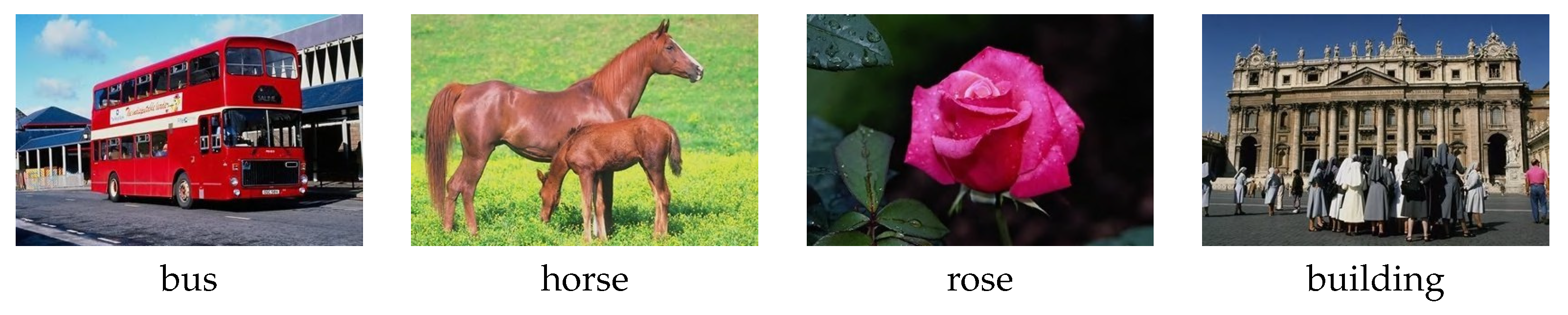
- The Wang database [30]: This image database collects 1000 images from the Corel photo stock database and consists of 100 images for 10 object classes {africa people, beaches, buildings, buses, dinosaurs, elephants, roses, horses, mountains, foods}. Figure 4 shows the four images out of this database.
To treat images in the compression-based pattern recognition, they must be converted to one-dimensional strings beforehand: First, we transform a pixel in an image into a character according to its Lab color in such a way that the Lab color space is quantized into 64 levels by dividing each color axis into four segments. Then, the image is represented as a string by concatenating the characters in the scanning of the image row by row. This way of raster-scan is called the Row-Major [31].
We implemented the whole of our method in C++ language with the g++ compiler. We wrote the program code of the LZW algorithm by ourselves. We relied on the C++ API of the OpenCV library to read images.
We measure the quality of a CV space with the preciseness of image classification that is evaluated with the leave-one-out method as follows. Let A and C be the number of images and class categories in the image database, respectively. For the UC Merced land use dataset, we have and , while and for the Wang database. A query image selected from the A images is classified into one of the C classes with the K-NN classifier that performs the K-NN similar image retrieval against the remaining images where . Let be the number of query images categorized into the ground-truth class. Then, the accuracy rate is defined as .
The maximum number of words in an LZW dictionary is set to 4096.
4.1. Comparison of Accuracy Rate
We compare the recognition accuracy rate between the raw base dictionaries created by the dictionary selection algorithm and those modified by our editing methods REVIVAL and VOCAB. The experiment procedure proceeds as follows: First, an arbitrary dictionary selection algorithm chooses the base dictionaries and lets them span the compression-based feature space. Then, REVIVAL and VOCAB modify the chosen base dictionaries and span the two other CV spaces with the modified dictionaries. Then, we compare the accuracy rate of CV space between the raw base dictionaries and those modified by our methods REVIVAL/VOCAB. To highlight the effect of word reassignment, we also prepare the base dictionaries which simply exclude the common words from the raw base dictionaries without reassigning words according to the procedure in Section 3.1. This method is named as “NO_COMMON”.
We implement the two dictionary selection algorithms in the literature, i.e., PRDC [6] and SUPERVISED [9]. Regarding PRDC, we let the temporal CV space have the same number of dimensions as the final CV space. According to the notations in Section 2.2, . On the other hand, SUPERVISED is implemented in such a way that the N base dictionaries are derived by randomly gathering objects per class.
Figure 5 shows the accuracy rates achieved by various base dictionaries for the UC MERCED dataset, when the dictionary selection algorithm is PRDC. In this graph, the raw base dictionaries are assigned a legend “PRDC”. Figure 6 presents the result when the dictionary selection algorithm is SUPERVISED. Again, the raw base dictionaries are assigned a legend “SUPERVISED”. Here, we vary N, and the number of base dictionaries is in the range from 5 to 35. Since both PRDC and SUPERVISED are randomized algorithms, the average values over 10 trials are plotted.
In both of the graphs, REVIVAL, VOCAB, and NO_COMMON are more accurate than the raw base dictionaries except for the only case when for VOCAB. Thus, our approach to raise the independence among the base dictionaries by prohibiting any common words definitely enhances the quality of the CV spaces.
For instance, for , the accuracy rate becomes 0.747 for REVIVAL, while PRDC attains the accuracy rate of 0.666. Therefore, the performance gain of REVIVAL relative to PRDC grows 11.2%. Similarly, the accuracy rates for REVIVAL and SUPERVISED become 0.735 and 0.676 when , so that the relative performance gain becomes 10.9%. Remarkably, PRDC and SUPERVISED are hard to increase the accuracy rate by augmenting the number of dimensions for . These results are interpreted as follows: The approach to choose various dictionaries based on the object-level dissimilarity fails to enrich the variety of chosen dictionaries for large N values, since many words are common to multiple dictionaries. By contrast, our method smartly keeps the dictionaries independent of one another even for large N values by imposing the constraint that any word belongs to only one dictionary. In fact, for , the 10 dictionaries hold about 26,900 words in total after the common words are removed, whereas they possess 40,960 words originally. Therefore, of the words in the dictionaries are redundant and deteriorate the independence among dimensions.
Next, NO_COMMON is always defeated by REVIVAL except when the dictionary selection algorithm is PRDC and . This result can be explained in the following way: As stated in Section 3.2, in NO_COMMON, a base dictionary stores a few words, if i is sufficiently large. Since such cannot compress objects well, the dimension associated with does not have rich expressive ability and is dominated by other dimensions with smaller subscripts. To illustrate the above situation comprehensively, we examine the variance over 500 compression vectors calculated from the 500 images in the UC Merced dataset per dimension. The two pie charts in Figure 7 summarize the variance of each dimension for REVIVAL and NO_COMMON, when . Starting from the top, the pie charts arrange the variances of all the dimensions in counterclockwise order. For NO_COMMON, the variance of almost monotonically decreases as i augments. The reason why the variance becomes low is that the compression ratio becomes large and close to 1 for many objects. Thus, for instance, , , and have by far larger variances than the last 10 dictionaries and dominate them in compression vectors. Thus, the backward dimensions are not very useful for pattern recognition. By contrast, REVIVAL suppresses such dimensions whose variances are extremely high or low, since all the dictionaries have the same number of words. Thus, the dimensions in the CV space cooperate better in REVIVAL than in NO_COMMON.
Finally, REVIVAL outperforms VOCAB for the UC Merced Dataset. This result implies that the base dictionaries are desirable to retain the structure of raw base dictionaries derived from real objects rather than to destroy it completely. We will discuss this point later after reporting the recognition accuracy for the Wang database.
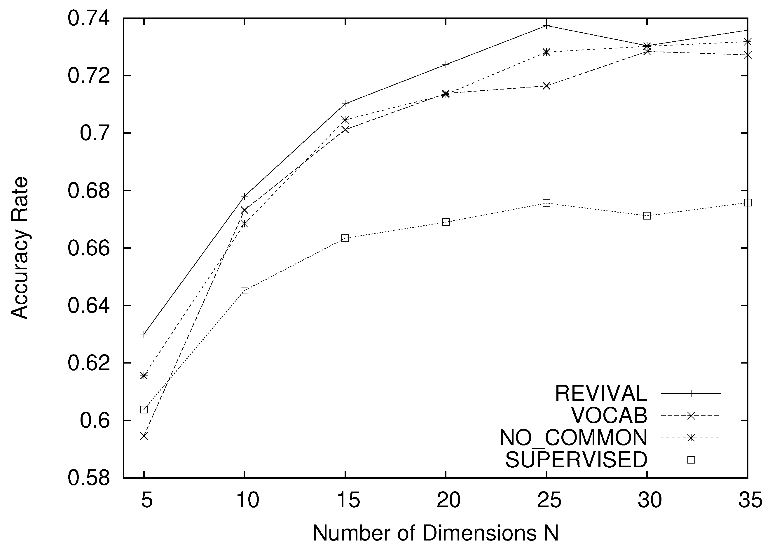
For the Wang database, Figure 8 and Figure 9 illustrate the accuracy rate when the dictionary selection algorithm is PRDC and SUPERVISED, respectively. To obtain exactly the same number of base dictionaries from the 10 object classes, N is set to be a multiple of 10, when we deal with SUPERVISED. In the same way as the UC Merced dataset,
- REVIVAL, VOCAB and NO_COMMON evidently achieve higher accuracy rates for any N than the raw base dictionaries.
- REVIVAL outperforms NO_COMMON regardless of the dictionary selection algorithm.
However, this experiment gets one significant difference from the result with the UC Merced dataset: VOCAB is the most accurate and excels to REVIVAL. We consider that this difference is attributed to the nature of the pattern recognition task. For the UC Merced dataset, we need to infer the class of land cover. This recognition task is very similar to texture recognition. Thus, every part of an image is uniformly useful for class recognition. On the other hand, the Wang database demands to recognize objects such as horses, elephants, buildings, roses, foods, and buses. An image with an instance of these classes usually consists of the foreground and the background as in Figure 4, and only the foreground is the objective of recognition. Here, a compression dictionary , which LZW generates from , mixes the words from ’s foreground region and those from ’s background region. Then, even if compresses a test image well, it does not always mean that ’s foreground does exist in because it is possible that contains ’s background only. In this way, is not optimized for the detection of ’s foreground. REVIVAL and NO_COMMON inherit this property, since they try to retain the structure of . VOCAB uses a base dictionary which collects words whose prefixes are similar. In the context of image processing, words with similar prefixes correspond to pixel sequences with similar colors. Thus, the base dictionaries in VOCAB are tailored to recognize the foreground or the foreground component of a uniform color. After all, VOCAB works accurately, since some dimensions in the CV can measure the likelihood of existence for the foreground (or foreground components).
Thus, the experimental results for our two datasets indicate that the optimal construction of base dictionaries depends on the recognition task.
4.2. Independence among Feature Dimensions
Regarding REVIVAL and PRDC, we evaluate how the feature dimensions are correlated quantitatively with the UC Merced dataset. For , we first generate the compression-ratio vectors for all the 500 images. Then, we compute the Pearson correlation coefficients between the two dimensions i and j satisfying from the i-th coordinate values and the j-th coordinate values for the 500 CVs. The matrix in Table 2 summarizes the result where the element shows the absolute value of the correlation coefficient between the two dimensions i and j. In particular, the upper-right triangle submatrix displays the correlation coefficients for REVIVAL, whereas the lower-left triangle submatrix lists those for PRDC. This matrix reports the experimental result of a typical single trial. The matrix elements greater than 0.6 are written in boldface. Obviously, there are more figures in boldface in the lower-left submatrix than in the upper-left submatrix, which means that more dimension pairs are correlated in PRDC than in REVIVAL. The average value of correlation coefficients over all dimension pairs becomes 0.401 for PRDC and 0.320 for REVIVAL. Thus, we suppose that the high accuracy rate of REVIVAL is gained by increasing the independence among feature dimensions.
4.3. Execution Time
We evaluate how efficient our method becomes by comparing the execution time for the UC Merced dataset between REVIVAL and PRDC. The experimental platform is a PC with Intel Core i7-3770 CPU @3.40 GHz, 16 GB memory Fixing N to 20, we report the execution time for the next four procedures in Table 3.
- (Procedure 1) PRDC chooses the N base dictionaries at the beginning.
- (Procedure 2) modifies the N dictionaries in D.
- (Procedure 3) After the N dictionaries are determined, the CVs are generated for all the objects in the UC Merced Dataset.
- (Procedure 4) classifies every object in the dataset with the K-NN classifier in the leave-one-out manner.
Note that (Procedure 2) is necessary only for REVIVAL, and PRDC skips it. The other three procedures are performed by both REVIVAL and PRDC.
From Table 3, we can see that (Procedure 1) and (Procedure 3) dominate the total execution time. These two procedures are quite time-consuming, as they perform the LZW data compression many times. For example, to generate 20-dimensional CVs for the 500 objects in the UC Merced Dataset, we must repeat the LZW data compression 10,000 times. While the total execution time of REVIVAL is not very different from that of PRDC, the cost of our dictionary editing in (Procedure 2) is negligible relative to that of data compression in (Procedure 1) and (Procedure 3).
5. Conclusions
This paper studies the CV (compression-ratio vector) space for compression-based pattern recognition. We present a technique to modify the given base dictionaries which form the dimensions of the CV space. In particular, we edit the base dictionaries so that any two different base dictionaries never may have any common words. This technique increases the independence among the dimensions and raises the quality of the CV space. Although the above idea is quite natural, it has not been addressed so far in the research area of compression-based pattern recognition whose original concept is to evaluate the similarity between two real objects with the compression ratio. We break away from this concept and dare to modify the base dictionaries in order to make a refined CV space. To further improve the recognition accuracy, we also adjust the assignment of words to dictionaries after removing common words. In particular, we invent two methods REVIVAL and VOCAB. Whereas REVIVAL maintains the structure of raw base dictionaries which LZW extracts by compressing real objects to some extent, VOCAB dares to discard it completely.
In the application to image classification, our approach to eliminate common words from the base dictionaries achieved higher recognition accuracy than the base case without it. We confirmed that our method surely reduces the correlation coefficients among the dimensions of the CV space. We also showed that the word reassignment can improve the recognition accuracy as compared with the approach to simply delete common words. The experimental results with two image datasets show that the optimal word reassignment depends on the pattern recognition task.
An important future work of this research is to pursue the relation between the optimal word reassignment and the given dataset. Another research direction is to give a theoretical analysis, which explains the reason why our algorithm works well.
Author Contributions
Algorithm design and project administration: H.K., software implementation and experimental evaluation: S.O. and Y.N. All authors have read and agreed to the published version of the manuscript.
Funding
This work is supported by the Ministry of Education, Culture, Sports, Science and Technology, Grant-in-Aid for Scientific Research (C) 15K00148.
Institutional Review Board Statement
Not applicable.
Informed Consent Statement
Not applicable.
Data Availability Statement
For experimental evaluation, we used two datasets open to the public: Refer to http://weegee.vision.ucmerced.edu/datasets/landuse.html (accessed on 9 June 2022) to find the UC Merced Land Use dataset and to http://wang.ist.psu.edu/docs/related/ (accessed on 9 June 2022) to access the Wang dataset.
Conflicts of Interest
The authors declare no conflict of interest.
References
- Li, M.; Chen, X.; Li, X.; Ma, B.; Vitanyi, P. The Similarity Metric. IEEE Trans. Inf. Theory 2004, 50, 3250–3264. [Google Scholar] [CrossRef]
- Luxburg, U. A Tutorial on Spectral Clustering. Stat. Comput. 2007, 17, 395–416. [Google Scholar] [CrossRef]
- Cilibrasi, R.L.; Vitányi, P.M. A Fast Quartet tree heuristic for hierarchical clustering. Pattern Recognit. 2011, 44, 662–677. [Google Scholar] [CrossRef] [Green Version]
- Cristianini, N.; Ricci, E. Support Vector Machines. In Encyclopedia of Algorithms; Kao, M.Y., Ed.; Springer: Boston, MA, USA, 2008; pp. 928–932. [Google Scholar] [CrossRef]
- Cilibrasi, R.; Vitanyi, P. Clustering by compression. IEEE Trans. Inf. Theory 2005, 51, 1523–1545. [Google Scholar] [CrossRef] [Green Version]
- Watanabe, T.; Sugawara, K.; Sugihara, H. A new pattern representation scheme using data compression. IEEE Trans. Pattern Anal. Mach. Intell. 2002, 24, 579–590. [Google Scholar] [CrossRef]
- Koga, H.; Nakajima, Y.; Toda, T. Effective construction of compression-based feature space. In Proceedings of the 2016 International Symposium on Information Theory and Its Applications (ISITA), Monterey, CA, USA, 30 October–2 November 2016; pp. 116–120. [Google Scholar]
- Nishida, K.; Banno, R.; Fujimura, K.; Hoshide, T. Tweet Classification by Data Compression. In Proceedings of the 2011 International Workshop on DETecting and Exploiting Cultural diversity on the Social Web, Glasgow, UK, 24 October 2011; pp. 29–34. [Google Scholar] [CrossRef]
- Cilibrasi, R.; Vitányi, P.; De Wolf, R. Algorithmic Clustering of Music Based on String Compression. Comput. Music J. 2004, 28, 49–67. [Google Scholar] [CrossRef]
- Li, M.; Zhu, Y. Image Classification via LZ78 Based String Kernel: A Comparative Study. In Proceedings of the 10th Pacific-Asia Conference on Advances in Knowledge Discovery and Data Mining, Singapore, 9–12 April 2006; pp. 704–712. [Google Scholar] [CrossRef]
- Cerra, D.; Datcu, M. Expanding the Algorithmic Information Theory Frame for Applications to Earth Observation. Entropy 2013, 15, 407–415. [Google Scholar] [CrossRef]
- Borbely, R.S. On normalized compression distance and large malware. J. Comput. Virol. Hacking Tech. 2015, 12, 235–242. [Google Scholar] [CrossRef] [Green Version]
- Hagenauer, J.; Mueller, J. Genomic analysis using methods from information theory. Proceedings of IEEE Information Theory Workshop, San Antonio, TX, USA, 24–29 October 2004; pp. 55–59. [Google Scholar]
- Sculley, D.; Brodley, C.E. Compression and Machine Learning: A New Perspective on Feature Space Vectors. In Proceedings of the Data Compression Conference, Snowbird, UT, USA, 28–30 March 2006; p. 332. [Google Scholar] [CrossRef] [Green Version]
- Macedonas, A.; Besiris, D.; Economou, G.; Fotopoulos, S. Dictionary Based Color Image Retrieval. J. Vis. Commun. Image Represent. 2008, 19, 464–470. [Google Scholar] [CrossRef]
- Cerra, D.; Datcu, M. A fast compression-based similarity measure with applications to content-based image retrieval. J. Vis. Commun. Image Represent. 2012, 23, 293–302. [Google Scholar] [CrossRef] [Green Version]
- Welch, T. A Technique for High-Performance Data Compression. Computer 1984, 17, 8–19. [Google Scholar] [CrossRef]
- Besiris, D.; Zigouris, E. Dictionary-based color image retrieval using multiset theory. J. Vis. Commun. Image Represent. 2013, 24, 1155–1167. [Google Scholar] [CrossRef]
- Uchino, T.; Koga, H.; Toda, T. Improved Compression-Based Pattern Recognition Exploiting New Useful Features. In Pattern Recognition and Image Analysis; Springer International Publishing: Cham, Switzerland, 2017; pp. 363–371. [Google Scholar]
- Field, R.; Quach, T.T.; Ting, C. Efficient Generalized Boundary Detection Using a Sliding Information Distance. IEEE Trans. Signal Process. 2020, 68, 6394–6401. [Google Scholar] [CrossRef]
- Zhang, N.; Watanabe, T. Topic Extraction for Documents Based on Compressibility Vector. IEICE Trans. 2012, 95-D, 2438–2446. [Google Scholar] [CrossRef] [Green Version]
- Cilibrasi, R. Statistical Inference Through Data Compression. Ph.D. Thesis, Institute for Logic, language and Computation, Universiteit van Amsterdam, Amsterdam, The Netherlands, 2007. [Google Scholar]
- Ting, C.; Field, R.; Fisher, A.; Bauer, T. Compression Analytics for Classification and Anomaly Detection Within Network Communication. IEEE Trans. Inf. Forensics Secur. 2019, 14, 1366–1376. [Google Scholar] [CrossRef]
- Casella, G.; Berger, R. Statistical Inference; Duxbury Resource Center: Duxbury, MA, USA, 2001. [Google Scholar]
- Coltuc, D.; Datcu, M.; Coltuc, D. On the Use of Normalized Compression Distances for Image Similarity Detection. Entropy 2018, 20, 99. [Google Scholar] [CrossRef] [PubMed] [Green Version]
- Ting, C.; Johnson, N.; Onunkwo, U.; Tucker, J.D. Faster classification using compression analytics. In Proceedings of the 2021 International Conference on Data Mining Workshops (ICDMW), Auckland, New Zealand, 7–10 December 2021; pp. 813–822. [Google Scholar] [CrossRef]
- Contreras, I.; Arnaldo, I.; Krasnogor, N.; Hidalgo, J.I. Blind optimisation problem instance classification via enhanced universal similarity metric. Memetic Comput. 2014, 6, 263–276. [Google Scholar] [CrossRef]
- Jolliffe, I.T. Principal Component Analysis; Springer: Berlin, Germany; New York, NY, USA, 1986. [Google Scholar]
- Yang, Y.; Newsam, S. Bag-of-visual-words and Spatial Extensions for Land-use Classification. In Proceedings of the 18th SIGSPATIAL International Conference on Advances in Geographic Information Systems, San Jose, CA, USA, 2–5 November 2010; pp. 270–279. [Google Scholar] [CrossRef]
- Wang, J.; Li, J.; Wiederhold, G. SIMPLIcity: Semantics-Sensitive Integrated Matching for Picture LIbraries. IEEE Trans. Pattern Anal. Mach. Intell. 2001, 23, 947–963. [Google Scholar] [CrossRef] [Green Version]
- Mortensen, J.; Wu, J.; Furst, J.; Rogers, J.; Raicu, D. Effect of Image Linearization on Normalized Compression Distance. In Signal Processing, Image Processing and Pattern Recognition; Springer: Berlin/Heidelberg, Germany, 2009; Volume 61, pp. 106–116. [Google Scholar]
Figure 1.
Our proposed method.

Figure 2.
Trie representing a modified dictionary.

Figure 3.
UC Merced land use dataset.

Figure 4.
Wang database.

Figure 5.
Accuracy rate for UC Merced land use dataset: PRDC.

Figure 6.
Accuracy rate for UC Merced land use dataset: SUPERVISED.

Figure 7.
Variance of coordinate values in compression-ratio vectors per dimension: Comparison between REVIVAL and NO_COMMON. For NO_COMMON, more dimensions take very small variances and are not descriptive than REVIVAL.
Figure 7.
Variance of coordinate values in compression-ratio vectors per dimension: Comparison between REVIVAL and NO_COMMON. For NO_COMMON, more dimensions take very small variances and are not descriptive than REVIVAL.

Figure 8.
Accuracy rate for Wang database: PRDC.

Figure 9.
Accuracy rate for Wang database: SUPERVISED.


Table 1.
Datasets in our experiments.
| Dataset | UC Merced Land Use | Wang |
|---|---|---|
| Number of images | 500 | 1000 |
| Number of classes | 5 | 10 |
| Class Name | ||
| 1 | forest | africa people |
| 2 | river | beaches |
| 3 | intersection | buildings |
| 4 | denseresidential | buses |
| 5 | building | dinosaurs |
| 6 | elephants | |
| 7 | roses | |
| 8 | horses | |
| 9 | mountains | |
| 10 | foods | |
Table 2.
Correlation coefficient between feature dimensions (absolute values); upper-right triangle submatrix: REVIVAL, lower-left triangle submatrix: PRDC.
Table 2.
Correlation coefficient between feature dimensions (absolute values); upper-right triangle submatrix: REVIVAL, lower-left triangle submatrix: PRDC.
| 0.340 | 0.508 | 0.160 | 0.581 | 0.598 | 0.530 | 0.496 | 0.463 | 0.173 | ||
| 0.011 | 0.509 | 0.536 | 0.824 | 0.114 | 0.218 | 0.045 | 0.275 | 0.213 | ||
| 0.285 | 0.714 | 0.016 | 0.516 | 0.455 | 0.187 | 0.359 | 0.218 | 0.484 | ||
| 0.199 | 0.387 | 0.118 | 0.539 | 0.242 | 0.234 | 0.148 | 0.142 | 0.120 | ||
| 0.214 | 0.878 | 0.843 | 0.238 | 0.288 | 0.453 | 0.046 | 0.322 | 0.175 | ||
| 0.540 | 0.074 | 0.143 | 0.476 | 0.168 | 0.664 | 0.133 | 0.675 | 0.252 | ||
| 0.081 | 0.649 | 0.832 | 0.006 | 0.810 | 0.217 | 0.170 | 0.740 | 0.061 | ||
| 0.650 | 0.268 | 0.160 | 0.116 | 0.114 | 0.718 | 0.166 | 0.217 | 0.045 | ||
| 0.357 | 0.374 | 0.314 | 0.174 | 0.272 | 0.815 | 0.146 | 0.831 | 0.001 | ||
| 0.386 | 0.650 | 0.585 | 0.160 | 0.648 | 0.361 | 0.725 | 0.591 | 0.563 |
Table 3.
Comparison of execution time between REVIVAL and PRDC.
| REVIVAL | PRDC | |
|---|---|---|
| (1) Selection of Initial Base Dictionaries [ms] | 23,551 | 23,516 |
| (2) Dictionary Modification [ms] | 342 | 0 |
| (3) Generation of CVs [ms] | 25,734 | 24,358 |
| (4) Object Classification [ms] | 57 | 56 |
Publisher’s Note: MDPI stays neutral with regard to jurisdictional claims in published maps and institutional affiliations. |
© 2022 by the authors. Licensee MDPI, Basel, Switzerland. This article is an open access article distributed under the terms and conditions of the Creative Commons Attribution (CC BY) license (https://creativecommons.org/licenses/by/4.0/).
Share and Cite
MDPI and ACS Style
Koga, H.; Ouchi, S.; Nakajima, Y. Editing Compression Dictionaries toward Refined Compression-Based Feature-Space. Information 2022, 13, 301. https://0-doi-org.brum.beds.ac.uk/10.3390/info13060301
AMA Style
Koga H, Ouchi S, Nakajima Y. Editing Compression Dictionaries toward Refined Compression-Based Feature-Space. Information. 2022; 13(6):301. https://0-doi-org.brum.beds.ac.uk/10.3390/info13060301
Chicago/Turabian StyleKoga, Hisashi, Shota Ouchi, and Yuji Nakajima. 2022. "Editing Compression Dictionaries toward Refined Compression-Based Feature-Space" Information 13, no. 6: 301. https://0-doi-org.brum.beds.ac.uk/10.3390/info13060301
Note that from the first issue of 2016, this journal uses article numbers instead of page numbers. See further details here.