

Wavelet-Based Classification of Enhanced Melanoma Skin Lesions through Deep Neural Architectures
 , , and
Abstract
:1. Introduction
2. Related Works
2.1. Need for the Study
2.2. Contribution of the Research Article
- (i)
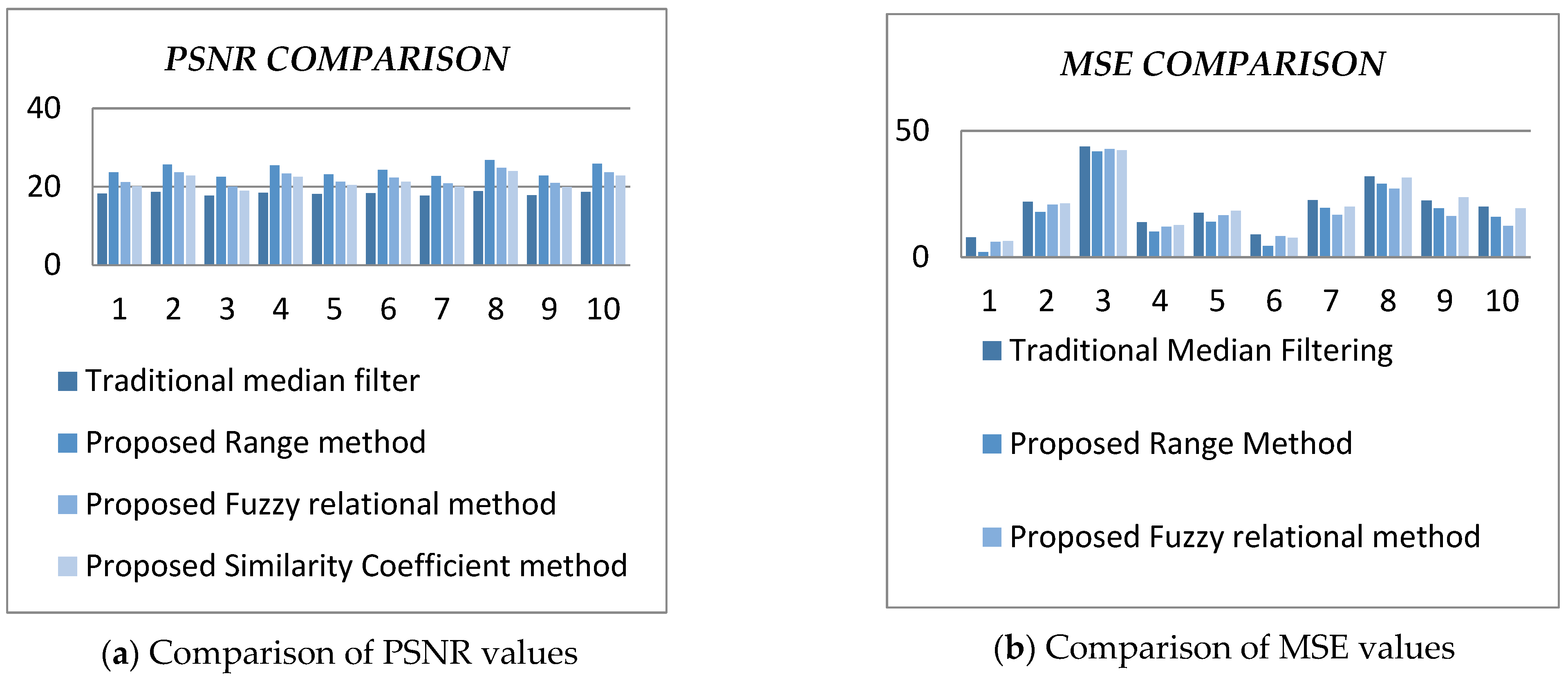
- A novel pre-processing method was used as a basis for median filtering. The traditional median filter was hybridized with the Range method (Algorithm 1), Fuzzy Relational method (Algorithm 2), and Similarity coefficient method (Algorithm 3);
- (ii)
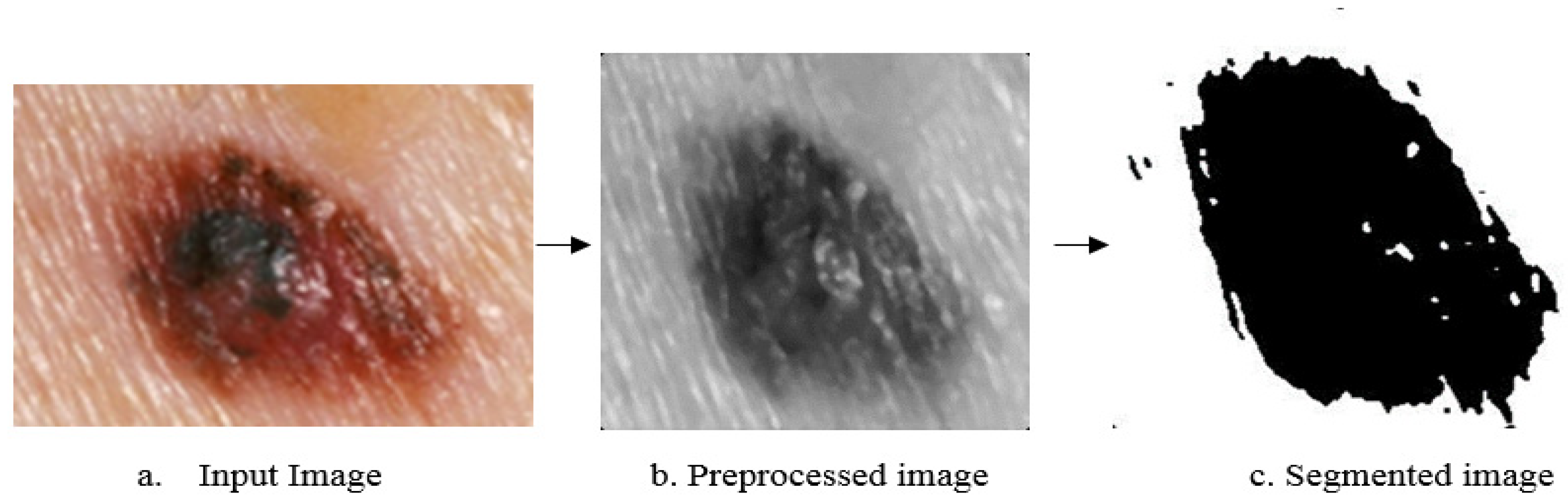
- Segmentation was imparted using Normalized Otsu’s segmentation [18];
- (iii)
- Feature extraction was performed with Wavelet coefficients (DB4, Symlets, RBIO);
- (iv)
- Classification was performed using ANN, SVM, and ANFIS. The proposed algorithms were implemented with melanoma skin lesion images and enhanced for further processing. The quality factor of the enhanced image was then measured with statistical measures such as Peak Signal to Noise Ratio (PSNR) and Mean Square Error (MSE).
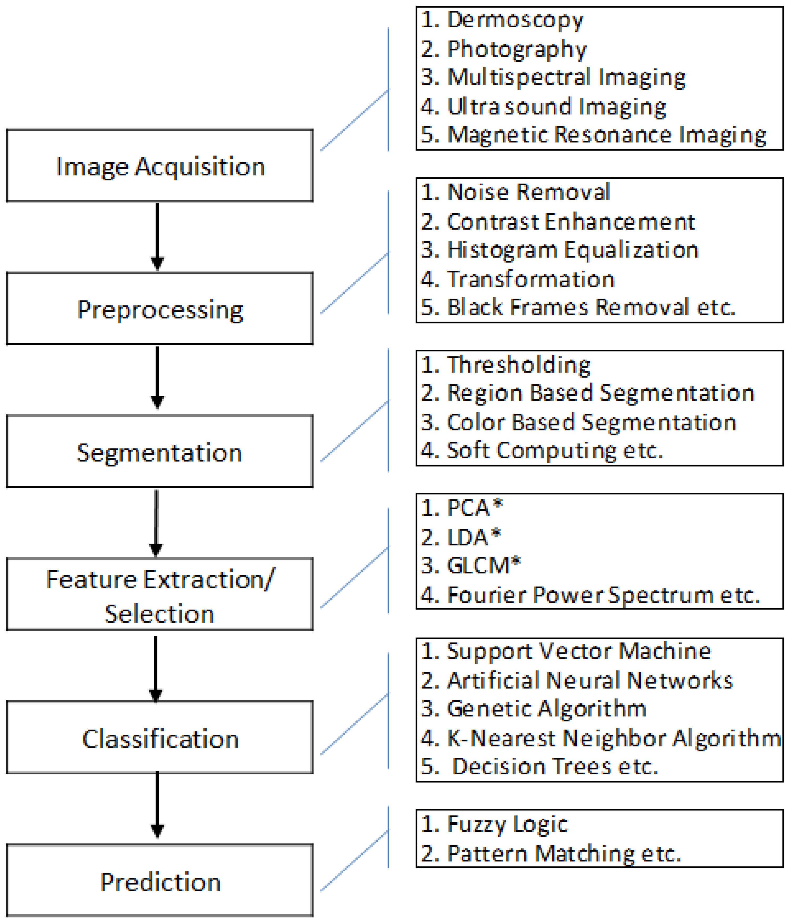
3. Proposed Methodology
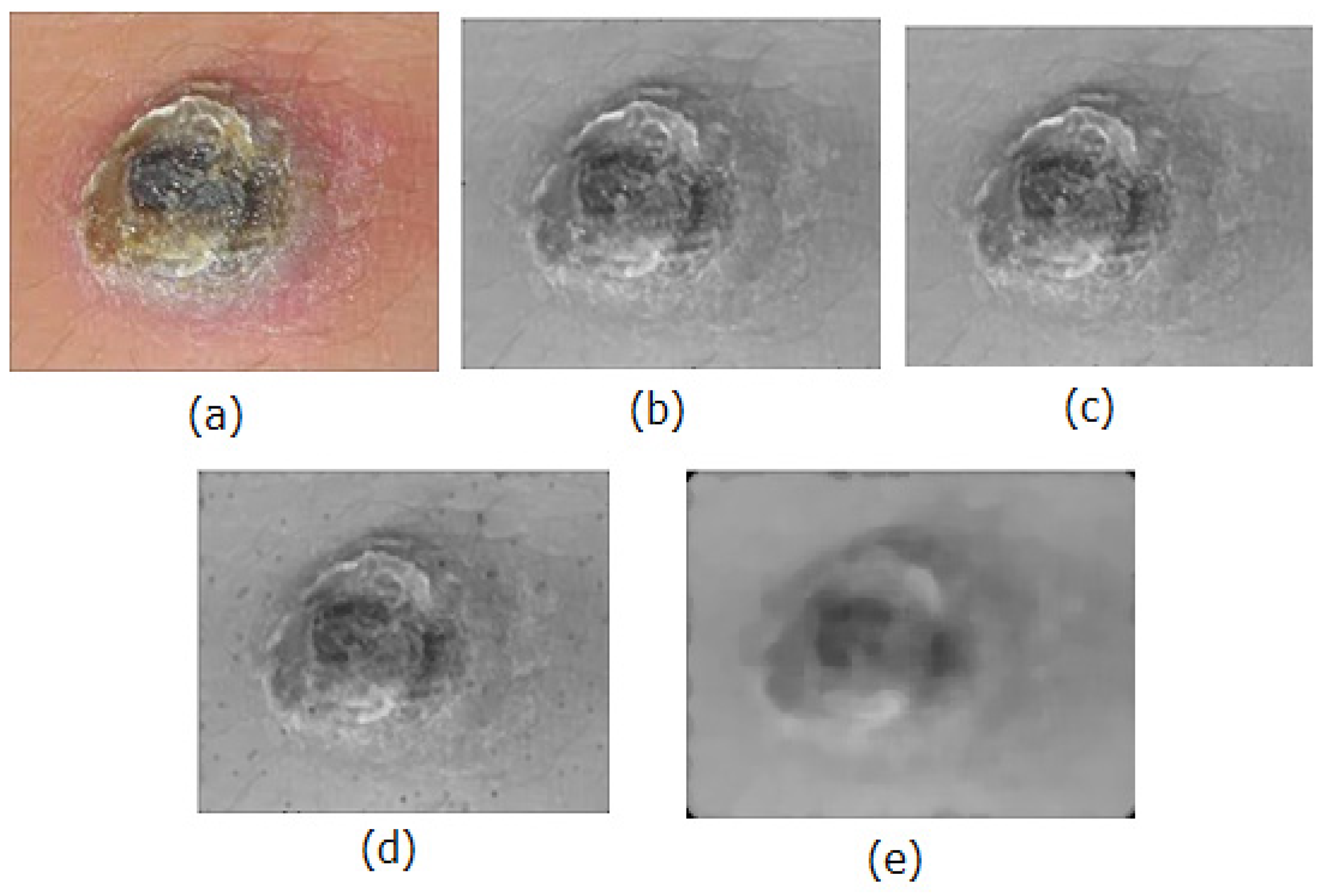
3.1. Image Enhancement through an Enhanced Median Filter
3.1.1. Algorithm for Range Method
| Algorithm 1: Range Method. |
| Input: Gray scale image of melanoma/benign skin lesion Output: Enhanced image
|
3.1.2. Algorithm for Fuzzy Relational Method
| Algorithm 2: Fuzzy Relational Method. |
| Input: Gray scale image of melanoma/benign skin lesion Output: Enhanced image
|
3.1.3. Algorithm for Similarity Coefficient Method
| Algorithm 3: Similarity Coefficient Method. |
| Input: Grayscale image of melanoma/benign skin lesion Output: Enhanced image
|
3.2. Segmentation
3.2.1. Entropy Features
3.2.2. Approximate Entropy (ApEn)
3.2.3. Sample Entropy (SamEn)
3.2.4. Shannon Entropy (ShEn)
3.2.5. Log Energy Entropy (LogEn)
3.2.6. Threshold Entropy (ThEn)
3.2.7. Sure Entropy (SrEn)
3.2.8. Norm Entropy (NmEn)
3.3. Statistical Features
- where i = matrix of low/high-frequency components, = matrix element, M × N is the size of the coefficient matrix.
- if the vector has an odd number of values. , where m, n = two mid values if the vector has an even number of values. The median of the matrix gives the central tendency of the matrix.
- Standard deviation , where m n = Window size, represent the Input of r rows and c columns.
- The median absolute deviation is the measure of average absolute deviations from a central point with respect to the median. It is defined as the where m(X) = median of the values in a matrix or dataset, = element of a matrix, and mn = total number of elements.
- Mean absolute deviation also provides the average absolute deviations from a central point with respect to the mean value of the matrix. It is defined as where m(X) = mean, = element of a matrix, mn = total number of elements.
- Mathematically, the Norm is the total length of all the vectors in a vector space or matrices. The higher the norm value, the bigger the matrix is. Here, L1 norm and L2 norm were derived for the wavelet coefficients.
- L1 norm is also called Sum Absolute Difference, and it is the difference between two vectors which can be defined as where x = elements of the vector and i = index value.
- L2 norm is generally called the Euclidean norm, and it gives the vector difference. It is a sum of squared difference denoted by x = elements of the vector, and i = index value. The range is the takeaway between the maximum and minimum value of the vector space, and it is defined by .
Feature Selection
3.4. Classification
ANFIS
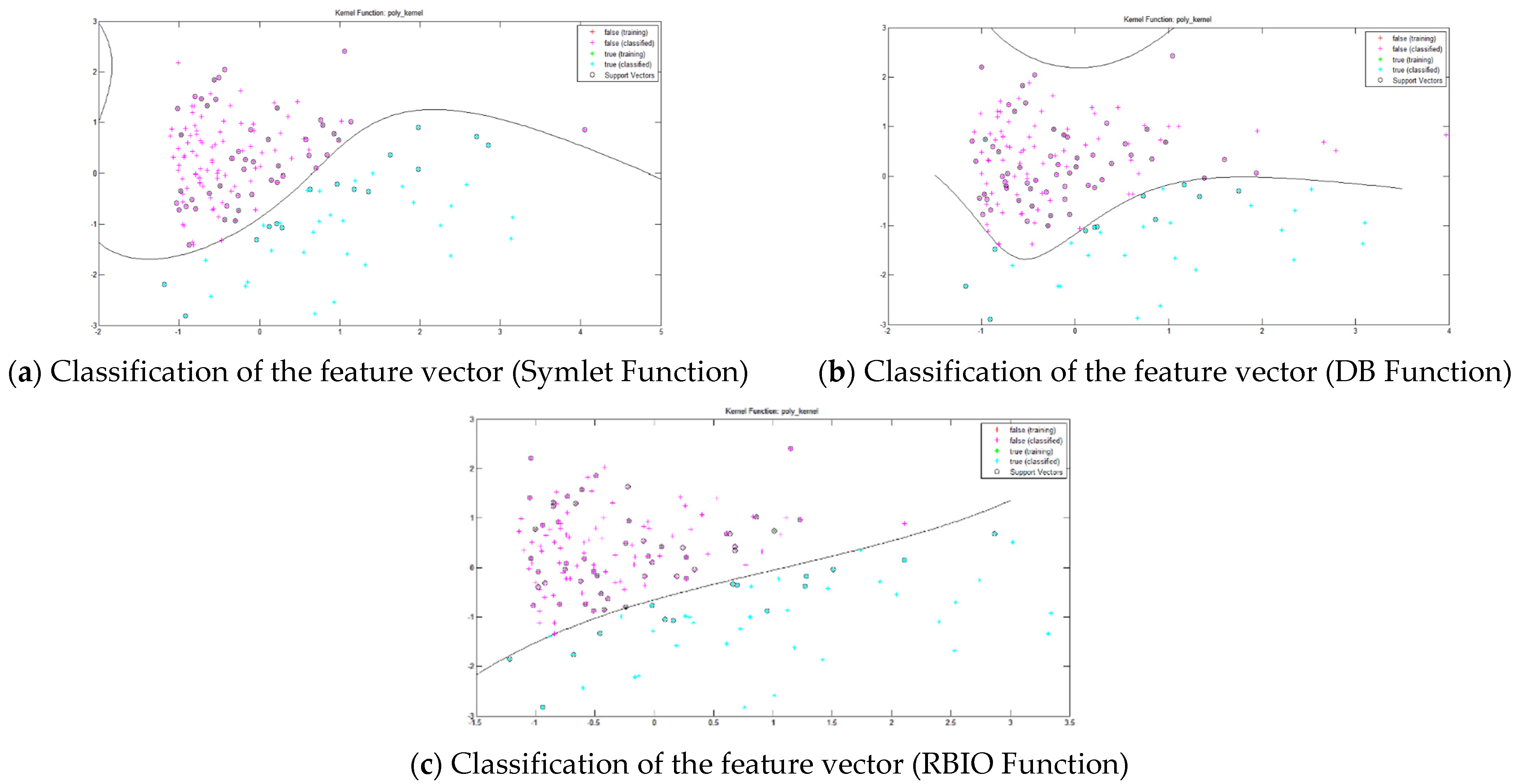
3.5. SVM
4. Experimentation Results
4.1. Normalized Otsu’s Segmentation
4.2. Discussion
- The classification accuracy obtained from DLNN through the Symlet function was higher than all other machine learning algorithms for the used dataset.
- Clearly, selecting entropy-based features yielded higher classification accuracy than selecting the mean and variance of the wavelet coefficients.
- We obtained a subtle difference (0.07%) between the spatial and frequency domain classification accuracy.
4.3. Limitations
5. Conclusions and Future Work
Author Contributions
Funding
Informed Consent Statement
Data Availability Statement
Acknowledgments
Conflicts of Interest
References
- Available online: http://www.cancer.org/cancer/skincancer-melanoma/detailedguide/melanoma-skin-cancer-key-statistics (accessed on 10 September 2021).
- Chatterjee, I. Artificial Intelligence and Patentability: Review and Discussions. Int. J. Mod. Res. 2021, 1, 15–21. [Google Scholar]
- Gupta, V.K.; Shukla, S.K.; Rawat, R.S. Crime tracking system and people’s safety in India using machine learning approaches. Int. J. Mod. Res. 2022, 2, 1–7. [Google Scholar]
- Gulati, S.; Bhogal, R.K. Classification of Melanoma from Dermoscopic Images Using Machine Learning. In Smart Intelligent Computing and Applications; Springer: Berlin/Heidelberg, Germany, 2020; pp. 345–354. [Google Scholar]
- Khan, M.A.; Sharif, M.; Akram, T.; Bukhari, S.A.; Nayak, R.S. Developed Newton-Raphson based deep features selection framework for skin lesion recognition. Pattern Recognit. Lett. 2020, 129, 293–303. [Google Scholar] [CrossRef]
- Rodrigues, D.D.; Ivo, R.F.; Satapathy, S.C.; Wang, S.; Hemanth, J.; Rebouças Filho, P.P. A new approach for classification skin lesion based on transfer learning, deep learning, and IoT system. Pattern Recognit. Lett. 2020, 136, 8–15. [Google Scholar] [CrossRef]
- Seeja, R.D.; Suresh, A. Deep Learning Based Skin Lesion Segmentation and Classification of Melanoma Using Support Vector Machine (SVM). Asian Pac. J. Cancer Prev. 2019, 20, 1555–1561. [Google Scholar]
- Abbas, Q.; Celebi, M.E. DermoDeep-A classification of melanoma-nevus skin lesions using multi-feature fusion of visual features and deep neural network. Multimed. Tools Appl. 2019, 78, 23559–23580. [Google Scholar] [CrossRef]
- Premaladha, J.; Ravichandran, K.S. Novel Approaches for Diagnosing Melanoma Skin Lesions through Supervised and Deep Learning Algorithms. J. Med. Syst. 2016, 40, 1–12. [Google Scholar] [CrossRef]
- Kruk, M.; Swiderski, B.; Osowski, S.; Kurek, J.; Słowińska, M.; Walecka, I. Melanoma recognition using extended set of descriptors and classifiers. EURASIP J. Image Video Process. 2015, 1, 1–10. [Google Scholar] [CrossRef] [Green Version]
- Premaladha, J.; Ravichandran, K.S. Detection of Melanoma Skin Lesions Using Phylogeny. Natl. Acad. Sci. Lett. 2015, 38, 333–338. [Google Scholar] [CrossRef]
- Alrashed, F.A.; Alsubiheen, A.M.; Alshammari, H.; Mazi, S.I.; Al-Saud, S.A.; Alayoubi, S.; Kachanathu, S.J.; Albarrati, A.; Aldaihan, M.M.; Ahmad, T.; et al. Stress, Anxiety, and Depression in Pre-Clinical Medical Students: Prevalence and Association with Sleep Disorders. Sustainability 2022, 14, 11320. [Google Scholar] [CrossRef]
- Premaladha, J.; Ravichandran, K.S. Quantification of Fuzzy Borders and Fuzzy Asymmetry of Malignant Melanomas. Proc. Natl. Acad. Sci. India Sect. A Phys. Sci. 2015, 85, 303–314. [Google Scholar]
- Schaefer, G.; Krawczyk, B.; Celebi, M.E.; Iyatomi, H. An ensemble classification approach for melanoma diagnosis. Memetic Comput. 2014, 6, 233–240. [Google Scholar]
- Liu, Z.; Sun, J.; Smith, L.; Smith, M.; Warr, R. Distribution quantification on dermoscopy images for computer-assisted diagnosis of cutaneous melanomas. Med. Biol. Eng. Comput. 2012, 50, 503–513. [Google Scholar] [CrossRef] [PubMed]
- Shukla, S.K.; Gupta, V.K.; Joshi, K.; Gupta, A.; Singh, M.K. Self-aware Execution Environment Model (SAE2) for the Performance Improvement of Multicore Systems. Int. J. Mod. Res. 2022, 2, 17–27. [Google Scholar]
- Sharma, T.; Nair, R.; Gomathi, S. Breast Cancer Image Classification using Transfer Learning and Convolutional Neural Network. Int. J. Mod. Res. 2022, 2, 8–16. [Google Scholar]
- Premaladha, J.; Priya, M.L.; Sujitha, S.; Ravichandran, K.S. Normalised Otsu’s Segmentation Algorithm for Melanoma Diagnosis. Indian J. Sci. Technol. 2015, 8, 1. [Google Scholar] [CrossRef]
- Janani, P.; Premaladha, J.; Ravichandran, K.S. Image Enhancement Techniques: A Study. Indian J. Sci. Technol. 2015, 8, 1–12. [Google Scholar] [CrossRef]
- Giotis, I.; Molders, N.; Land, S.; Biehl, M.; Jonkman, M.F.; Petkov, N. MED-NODE: A computer-assisted melanoma diagnosis system using non-dermoscopic images. Expert Syst. Appl. 2015, 42, 6578–6585. [Google Scholar]
- Yuan, X.; Martínez, J.-F.; Eckert, M.; López-Santidrián, L. An Improved Otsu Threshold Segmentation Method for Underwater Simultaneous Localization and Mapping-Based Navigation. Sensors 2016, 16, 1148. [Google Scholar] [CrossRef] [Green Version]
- Surowka, G. Symbolic learning supporting early diagnosis of melanoma. In Proceedings of the 2010 Annual International Conference of the IEEE Engineering in Medicine and Biology, Buenos Aires, Argentina, 31 August–4 September 2010; Volume 31, pp. 4104–4107. [Google Scholar]
- Surowka, G. Supervised learning of melanocytic skin lesion images. In Proceedings of the IEEE Conference on Human System Interactions, Kraków, Poland, 25–27 May 2008; pp. 121–125. [Google Scholar]
- Fassihi, N.; Shanbehzadeh, J.; Sarafzadeh, A.; Ghasemi, E. Melanoma diagnosis by the use of wavelet analysis based on morphological operators. In Proceedings of the International Multiconference of Engineers and Computer Scientists, Hong Kong, China, 16–18 March 2011; pp. 16–18. [Google Scholar]
- D’Alessandro, B.; Dhawan, A.P.; Mullani, N. Computer aided analysis of epi-illumination and transillumination images of skin lesions for diagnosis of skin cancers. In Proceedings of the 2011 Annual International Conference of the IEEE Engineering in Medicine and Biology Society, Boston, MA, USA, 30 August–3 September 2011; pp. 3434–3438. [Google Scholar]
- Garnavi, R.; Aldeen, M.; Bailey, J. Computer-aided diagnosis of melanoma using border-and wavelet-based texture analysis. IEEE Trans. Inf. Technol. Biomed. 2012, 16, 1239–1252. [Google Scholar]
- Pincus, S.M. Approximate entropy as a measure of system complexity. Proc. Natl. Acad. Sci. USA 1991, 88, 2297–2301. [Google Scholar] [CrossRef] [PubMed] [Green Version]
- Bruhn, J.; Ropcke, H.; Hoeft, A. Approximate entropy as an electroencephalographic measure of anesthetic drug effect during desflurane anesthesia. Anesthesiology 2001, 92, 715–726. [Google Scholar]
- Attallah, O.; Sharkas, M.A.; Gadelkarim, H. Deep Learning Techniques for Automatic Detection of Embryonic Neurodevelopmental Disorders. Diagnostics 2020, 10, 27. [Google Scholar] [CrossRef] [PubMed] [Green Version]
- Zhang, Z.; Pan, H.; Wang, X.; Lin, Z. Machine Learning-Enriched Lamb Wave Approaches for Automated Damage Detection. Sensors 2020, 20, 1790. [Google Scholar] [CrossRef] [Green Version]
- Richman, J.S.; Moorman, J.R. Physiological time series analysis using approximate entropy and sample entropy. Am. J. Physiol. Heart Circ. 2000, 278, H2039–H2049. [Google Scholar] [CrossRef] [Green Version]
- Shannon, C.E.; Weaver, W. The Mathematical Theory of Communication; University of Illinois Press: Champaign, IL, USA, 1964; pp. 1–117. [Google Scholar] [CrossRef] [Green Version]
- Coifman, R.R.; Wickerhauser, M.V. Entropy-based algorithms for best basis selection. IEEE Trans. Inf. Theory 1992, 38, 713–718. [Google Scholar] [CrossRef] [Green Version]
- Sabeti, M.; Katebi, S.; Boostani, R. Entropy and complexity measures for EEG signal classification of schizophrenic and control participants. Artif. Intell. Med. 2009, 47, 263–274. [Google Scholar] [CrossRef]
- Aydın, S.; Saraoglu, H.M.; Kara, S. Log energy entropy-based EEG classification with multilayer neural networks in seizure. Ann. Biomed. Eng. 2009, 37, 2626–2630. [Google Scholar]
- Avci, D. An expert system for speaker identification using adaptive wavelet sure entropy. Expert Syst. Appl. 2009, 36, 6295–6300. [Google Scholar]
- Turkoglu, I.; Arslan, A.; Ilkay, E. An Intelligent system for diagnosis of the heart valve diseases with wavelet packet natural Networks. Comput. Biol. Med. 2003, 33, 319–331. [Google Scholar] [CrossRef]
- Duda, R.; Hart, P.; Stork, D. Pattern Classification, 2nd ed.; John Wiley and Sons: New York, NY, USA, 2006; ISBN 978-0-471-05669-0. [Google Scholar]
- Premaladha, J.; Surendra Reddy, M.; Hemanth Kumar Reddy, T.; Sri Sai Charan, Y.; Nirmala, V. Recognition of Facial Expression Using Haar Cascade Classifier and Deep Learning. In Inventive Communication and Computational Technologies; Ranganathan, G., Fernando, X., Shi, F., Eds.; Lecture Notes in Networks and Systems; Springer: Singapore, 2022; Volume 311. [Google Scholar] [CrossRef]
- Codella, N.; Rotemberg, V.; Tschandl, P.; Celebi, M.E.; Dusza, S.; Gutman, D.; Helba, B.; Kalloo, A.; Liopyris, K.; Marchetti, M.; et al. Skin lesion analysis toward melanoma detection 2018: A challenge hosted by the international skin imaging collaboration (ISIC). arXiv 2019, arXiv:1902.03368. [Google Scholar]
- Mustafa, S.; Dauda, A.B.; Dauda, M. Image processing and SVM classification for melanoma detection. In Proceedings of the 2017 International Conference on Computing Networking and Informatics (ICCNI), Ota, Nigeria, 29–31 October 2017; pp. 1–5. [Google Scholar] [CrossRef]
- Kaur, R.; GholamHosseini, H.; Sinha, R.; Lindén, M. Melanoma Classification Using a Novel Deep Convolutional Neural Network with Dermoscopic Images. Sensors 2022, 22, 1134. [Google Scholar] [CrossRef] [PubMed]
- Iqbal, I.; Younus, M.; Walayat, K.; Kakar, M.U.; Ma, J. Automated multi-class classification of skin lesions through deep convolutional neural network with dermoscopic images. Comput. Med. Imaging Graph. 2021, 88, 101843. [Google Scholar] [CrossRef] [PubMed]
- Shukla, P.; Verma, A.; Abhishek Verma, S.; Kumar, M. Interpreting SVM for medical images using Quadtree. Multimed. Tools Appl. 2020, 79, 29353–29373. [Google Scholar] [CrossRef] [PubMed]
- Ahmad, F.; Shahid, M.; Alam, M.; Ashraf, Z.; Sajid, M.; Kotecha, K.; Dhiman, G. Levelized Multiple Workflow Allocation Strategy under Precedence Constraints with Task Merging in IaaS Cloud Environment. IEEE Access 2022, 10, 92809–92827. [Google Scholar] [CrossRef]
- Kumar, R.; Dhiman, G. A Comparative Study of Fuzzy Optimization through Fuzzy Number. Int. J. Mod. Res. 2021, 1, 1–14. [Google Scholar]
- Hosny, K.M.; Kassem, M.A.; Foaud, M.M. Classification of skin lesions using transfer learning and augmentation with Alex-net. PLoS ONE 2019, 14, e0217293. [Google Scholar] [CrossRef] [PubMed]


| Entropy Features | Statistical Features |
|---|---|
|
|
| Images | Traditional Median Filter | Range Method | Fuzzy Relational Method | Similarity Coefficient Method | ||||
|---|---|---|---|---|---|---|---|---|
| PSNR | MSE | PSNR | MSE | PSNR | MSE | PSNR | MSE | |
| 1.jpg | 18.21 | 7.78 | 23.63 | 2.04 | 21.13 | 6.04 | 20.15 | 6.44 |
| 2.jpg | 18.67 | 21.91 | 25.68 | 17.90 | 23.68 | 20.79 | 22.81 | 21.2 |
| 3.jpg | 17.74 | 43.67 | 22.52 | 41.73 | 20.02 | 42.71 | 18.97 | 42.23 |
| 4.jpg | 18.43 | 13.75 | 25.43 | 10.09 | 23.38 | 12.99 | 22.53 | 12.59 |
| 5.jpg | 18.10 | 17.46 | 23.09 | 13.99 | 21.29 | 16.55 | 20.42 | 18.39 |
| 6.jpg | 18.33 | 8.93 | 24.32 | 4.37 | 22.32 | 8.26 | 21.27 | 7.67 |
| 7.jpg | 17.74 | 22.60 | 22.68 | 19.39 | 20.88 | 16.72 | 20.03 | 19.89 |
| 8.jpg | 18.81 | 31.86 | 26.82 | 28.98 | 24.78 | 27.08 | 23.91 | 31.48 |
| 9.jpg | 17.77 | 22.33 | 22.77 | 19.26 | 20.97 | 16.26 | 19.92 | 23.66 |
| 10.jpg | 18.65 | 20.01 | 25.89 | 15.94 | 23.69 | 12.34 | 22.84 | 19.24 |
| S.no | Classification Technique | Accuracy (%) | Sensitivity (%) | Specificity (%) | Kappa (%) | Precision (%) | F1 Score (%) | Training Time (in Minutes) | Testing Time (in Seconds) | |
|---|---|---|---|---|---|---|---|---|---|---|
| 1. | SVM [41] | 80.00 | 86.29 | 55.36 | 73.05 | 86.21 | 71.43 | 46.42 | 379 | |
| 2. | DCNN [42] | 81.41 | 81.88 | 89.12 | 81.80 | 81.30 | 81.05 | 48.64 | 372 | |
| 3. | Neural Network [43] | 91.25 | 91.32 | 90.03 | 89.21 | 91.97 | 91.47 | 49.03 | 362 | |
| 4. | SVM QuadTree Tree [44] | 86.04 | 93.44 | 68.00 | 78.07 | 87.69 | 90.47 | 48.42 | 396 | |
| Proposed Methodologies | DB | ANN | 85.75 | 88.70 | 82.30 | 71.20 | 85.69 | 87.17 | 48.82 | 360 |
| ANFIS | 84.51 | 87.85 | 80.53 | 68.60 | 84.08 | 85.92 | 48.96 | 374 | ||
| SVM | 89.32 | 90.96 | 87.47 | 78.50 | 90.14 | 90.55 | 44.01 | 342 | ||
| DLNN | 86.50 | 88.85 | 83.63 | 72.70 | 86.94 | 87.88 | 38.99 | 264 | ||
| Real AdaBoost | 84.41 | 87.85 | 80.53 | 68.60 | 84.08 | 85.92 | 46.49 | 392 | ||
| Modest AdaBoost | 84.46 | 87.85 | 80.53 | 68.60 | 84.08 | 85.92 | 46.21 | 388 | ||
| Gentle AdaBoost | 87.62 | 89.93 | 84.98 | 75.10 | 87.99 | 88.95 | 45.95 | 372 | ||
| Hybrid AdaBoost | 90.24 | 91.99 | 88.04 | 80.20 | 90.50 | 91.24 | 46.36 | 391 | ||
| Symlet | ANN | 90.21 | 91.99 | 88.04 | 80.20 | 90.50 | 91.24 | 48.62 | 362 | |
| ANFIS | 89.41 | 90.96 | 87.47 | 78.50 | 90.14 | 90.55 | 48.92 | 381 | ||
| SVM | 89.92 | 91.32 | 87.03 | 79.30 | 90.50 | 90.99 | 44.21 | 333 | ||
| DLNN | 93.62 | 94.59 | 92.45 | 87.10 | 94.09 | 94.34 | 38.90 | 252 | ||
| Real AdaBoost | 86.73 | 89.17 | 83.67 | 73.00 | 86.94 | 88.04 | 46.81 | 382 | ||
| Modest AdaBoost | 87.04 | 88.95 | 84.77 | 73.80 | 87.99 | 88.47 | 46.49 | 372 | ||
| Gentle AdaBoost | 90.13 | 91.82 | 88.01 | 80.00 | 90.50 | 91.16 | 46.32 | 370 | ||
| Hybrid AdaBoost | 91.88 | 92.65 | 90.55 | 83.20 | 92.65 | 92.65 | 46.63 | 394 | ||
| RBIO | ANN | 86.39 | 89.11 | 83.11 | 72.50 | 86.40 | 87.74 | 49.02 | 359 | |
| ANFIS | 87.65 | 89.93 | 84.98 | 75.10 | 87.99 | 88.95 | 49.89 | 390 | ||
| SVM | 89.52 | 90.97 | 87.67 | 78.70 | 90.32 | 90.65 | 45.06 | 352 | ||
| DLNN | 89.44 | 90.96 | 87.47 | 78.50 | 90.14 | 90.55 | 39.04 | 277 | ||
| Real AdaBoost | 84.95 | 88.51 | 80.69 | 69.50 | 84.08 | 86.24 | 46.96 | 394 | ||
| Modest AdaBoost | 86.31 | 89.11 | 83.11 | 72.50 | 86.40 | 87.74 | 46.21 | 382 | ||
| Gentle AdaBoost | 89.69 | 90.97 | 87.67 | 78.70 | 90.32 | 90.65 | 47.33 | 399 | ||
| Hybrid AdaBoost | 90.17 | 91.82 | 88.01 | 80.00 | 90.50 | 91.16 | 47.04 | 401 | ||
Publisher’s Note: MDPI stays neutral with regard to jurisdictional claims in published maps and institutional affiliations. |
© 2022 by the authors. Licensee MDPI, Basel, Switzerland. This article is an open access article distributed under the terms and conditions of the Creative Commons Attribution (CC BY) license (https://creativecommons.org/licenses/by/4.0/).
Share and Cite
Jayaraman, P.; Veeramani, N.; Krishankumar, R.; Ravichandran, K.S.; Cavallaro, F.; Rani, P.; Mardani, A. Wavelet-Based Classification of Enhanced Melanoma Skin Lesions through Deep Neural Architectures. Information 2022, 13, 583. https://0-doi-org.brum.beds.ac.uk/10.3390/info13120583
Jayaraman P, Veeramani N, Krishankumar R, Ravichandran KS, Cavallaro F, Rani P, Mardani A. Wavelet-Based Classification of Enhanced Melanoma Skin Lesions through Deep Neural Architectures. Information. 2022; 13(12):583. https://0-doi-org.brum.beds.ac.uk/10.3390/info13120583
Chicago/Turabian StyleJayaraman, Premaladha, Nirmala Veeramani, Raghunathan Krishankumar, Kattur Soundarapandian Ravichandran, Fausto Cavallaro, Pratibha Rani, and Abbas Mardani. 2022. "Wavelet-Based Classification of Enhanced Melanoma Skin Lesions through Deep Neural Architectures" Information 13, no. 12: 583. https://0-doi-org.brum.beds.ac.uk/10.3390/info13120583