The (T, L)-Path Model and Algorithms for Information Dissemination in Dynamic Networks

1
College of Computational Science, Zhongkai University of Agriculture and Engineering, Guangzhou 510000, China
2
School of Data and Computer Science, Sun Yat-sen University, Guangzhou 510006, China
*
Author to whom correspondence should be addressed.
Information 2018, 9(9), 212; https://0-doi-org.brum.beds.ac.uk/10.3390/info9090212
Submission received: 5 July 2018
/
Revised: 16 August 2018
/
Accepted: 19 August 2018
/
Published: 24 August 2018
Abstract
:A dynamic network is the abstraction of distributed systems with frequent network topology changes. With such dynamic network models, fundamental distributed computing problems can be formally studied with rigorous correctness. Although quite a number of models have been proposed and studied for dynamic networks, the existing models are usually defined from the point of view of connectivity properties. In this paper, instead, we examine the dynamicity of network topology according to the procedure of changes, i.e., how the topology or links change. Following such an approach, we propose the notion of the “instant path” and define two dynamic network models based on the instant path. Based on these two models, we design distributed algorithms for the problem of information dissemination respectively, one of the fundamental distributing computing problems. The correctness of our algorithms is formally proved and their performance in time cost and communication cost is analyzed. Compared with existing connectivity based dynamic network models and algorithms, our procedure based ones are definitely easier to be instantiated in the practical design and deployment of dynamic networks.
1. Introduction
Due to the rapid development of wireless technologies, the dynamic network is attracting more and more attention from researchers on study of distributed computing theory. A dynamic network is the general abstraction of networks with frequent topology changes [1,2,3,4]. The instances of dynamic networks cover various types of wireless networks, such as mobile ad hoc networks (MANET), wireless sensor networks (WSN), and vehicular ad hoc networks (VANET).
To cope with frequent topology changes of dynamic networks, quite a lot of work has been studied, including new system models and distributed algorithms. Distributed algorithms are designed to directly solve fundamental distributed computing problems such as naming, counting, and information dissemination [5,6,7,8,9] in dynamic networks. System models define and constrain the behaviors of underlying nodes or processes in a distributed system via abstractive assumptions and properties. Such assumptions and constraints are the basis and fundament of distributed algorithms, because arbitrary dynamic changes without any constraints will cause the impossibility of provable correctness in any computing task [10].
Most dynamic network models are defined by examining the effect of topology changes on network connectivity [3,10]. More precisely, they are concerned about whether the network is connected under topology changes rather than how these changes occur. Such connectivity based models are reasonable and useful because distributed computing applications certainly rely on the connectivity properties of networks. Based on these connectivity models, quite a number of fundamental distributed computing problems have been solved, including information dissemination.
However, connectivity based models have their shortcomings. As aforementioned, these models define network dynamicity in the point of view of connectivity properties of the network against dynamic topology changes. That is, they concern about the “result” of topology changes rather than the “procedure” of changes. Such an approach makes connectivity based models cannot be easily mapped to practical networks because there is no clue about how the nodes or links may change. Then, how to deploy a network with connectivity models is difficult.
Although there are some graphs based dynamic network models considering the time property of links (i.e., edges in the graph) [11,12], these models just provide methods to represent the change of network topologies and do not define the assumptions/constraints on these changes. Consequently, dynamic graph models cannot provide the properties/assumptions necessary to solve distributed computing problems. Shang [13,14] introduces a class of evolving range-dependent random graphs that gives a tractable framework for modeling. Since a probability is associated with the link between two agents, the information dissemination algorithm cannot get accurate results based on these models.
In this paper, we consider filling in the gap of “procedure” based dynamic network models. We first propose the notion of the “instant path”, which is the abstraction of the communication path between network nodes. With such a notion, we define two dynamicity models, named (T, l)-path and (T, l)*-path. These new models describe the topology dynamicity in terms of the procedure of communication paths, including node join and leave. Such models are more easily to be examined and observed in a real deployment of dynamic networks. With the new dynamic network models, we design several distributed algorithms for information dissemination.
Information dissemination is one of the fundamental problems in distributed computing, which is concerned with how to disseminate information to all the nodes in the network, with as little time cost and communication cost as possible [8,9]. The information dissemination problem is usually formalized as the k-token dissemination problem [10], where there are k tokens initially held by one or more network nodes and these tokens are finally disseminated to all nodes in the network.
Due to frequent topology changes, information dissemination or token dissemination in dynamic networks is much more challenging than in traditional network environments. Since information dissemination is a key fundamental problem in distributed computing, lots of work has been done for information dissemination in dynamic networks, and quite a number of algorithms have been designed for this problem [15,16,17]. However, all existing information dissemination algorithms assume connectivity based models, and consequently face the same problem of these models, i.e., they are difficult to be instantiated and observed in practical deployment.
Our proposed information dissemination algorithms are based on our new dynamic network models. We consider both 1-token dissemination and k-token dissemination, under the two models, respectively. Therefore, there are, in total, four algorithms proposed. The correctness of all the algorithms is formally proved and their performances in time cost and communication cost are analyzed.
The rest of the paper is organized as follows. Section 2 briefly reviews existing work on dynamic networks, including dynamic network models and information dissemination algorithms. The k-token problem and underlying system model are described in Section 3. In Section 4, we propose the concept of the instant path, and new dynamic network models, (T, l)-path and (T, l)*-path, and discusses relationships among different models. The algorithms based on the two models are presented in Section 5 and Section 6, respectively. Correctness proof together with cost analysis is presented following the description of each algorithm. Finally, Section 7 concludes the paper with future directions.
2. Related Work
Existing work on dynamic networks covers two major issues: dynamic network models and distributed algorithms. In this section, we first introduced the existing dynamic network models, and then reviewed existing algorithms for information dissemination in dynamic networks.
2.1. Dynamic Network Models
As aforementioned, existing dynamic network models describe network dynamicity according to either connectivity or the graph of the topology.
Graph-based dynamic network models are usually defined by extending the classical G(V, E) model [10], where V is the set of nodes in the network and E is the set of edges among the network nodes. By adding parameters to show topology dynamicity, Kempe et al. [11] proposed the temporal network model (G, λ), where λ is a set of labels to specify the time at which each edge e is available. Some researchers [2] view the dynamic network as the evolution of a topology graph consisting of a sequence of static graphs. Grindrod et al. [1] also adopted the view of graph evolution and defined a class of evolving range-dependent random graphs. Further, Clementi et al. [18] proposed Edge-Markovian dynamic graph, which considers the stochastic time-dependency in evolving graphs. Shang [19,20] studied the Estrada index of evolving graphs, and used linear algebra techniques to established general upper and lower bounds for these graph-spectrum based invariants through a couple of intuitive graph-theoretic measures, including the number of vertices or edges. Casteigts et al. [12] described the Time-Varying Graph (TVG) to integrate previous dynamic graph models, which present dynamic network as G = (V, E, T, ρ, ζ), where T is the lifetime of the network, ρ indicates whether a given edge is available, and ζ represents the time taken to cross an edge. By introducing two new elements C (the status of the node) and I (the cluster that the node belongs to), we extended the TVG to the cluster-based dynamic network in our previous work [13].
Obviously, these graph models mostly focus on how to represent the dynamic changing edges/links in a network rather than defining/constraining the behaviors of the network. Consequently, such models cannot be directly used to design fundamental distributed algorithms like information dissemination. Although the Edge-Markovian Graph [18] models the procedure of edge changes, the stochastic approach makes it not feasible for the design of distributed algorithms pursuing provable correctness. Wehmuth et al. [21] proposed the MultiAspect Graph (MAG) as a graph generalization, which considers the set of vertices, layers, time instants, or any other independent features as an aspect of the MAG.
Connectivity bases dynamic network models examine topology dynamicity according to the effect of topology changes on network connectivity. Kuhn et al. [6] proposed the notion of dynamic diameter, which can be used to describe the connectivity changes in the view of network diameter. The T-interval connected model is defined by Kuhn et al. [10]. It requires that, for every T consecutive rounds, there exists a stable connected spanning subgraph in the network. Ahmadi et al. [22] proposed the T-interval k-connected model, that is, for every interval of T consecutive rounds, there exists a k-vertex-connected stable subgraph.
Differing from Reference [10], in our previous work [13], we extended the existing dynamic network models with clusters, which was named (T, L)-HiNet model. (T, L)-HiNet includes several properties defining the stability of cluster hierarchy in a dynamic network, including the cluster head set, cluster member set and the connections among them. In our previous work [23], we proposed the (Q, S)-distance model, which is used to describe dynamic changes of information propagation time between any two nodes.
This connectivity based models put constraints on the connectivity of the network and can be easily adopted in distributed algorithm design. However, such models cannot be easily instantiated and overserved in real deployments because they are not concerned about the procedure of topology changes. Although Avin et al. [16] considered the topology change procedure, they assume that the topology changes only occur once within every certain number of rounds, which is too strong and not general enough. Such observations motivate us to pursue a dynamic network model defined according to the procedure of the topology changes.
2.2. Information Dissemination Algorithms
Information dissemination is one of the fundamental problems in distributed computing. Most information dissemination algorithms are designed for traditional static network environments.
To handle topology changes in dynamic networks, information dissemination is usually conducted by flooding or similar approaches [24]. By flooding, information dissemination in dynamic networks can be completed in O(n) if the network is always connected [10]. Baumann et al. [14] proposed the k-active flooding protocol, where each node forwards tokens for k times to propagate information fast. Kuhn et al. [10] designed a k-token dissemination algorithm based on the T-interval connectivity model. The algorithm consists of phases, each consisting of T rounds. In every round, each node generates a message to be delivered to all its current neighbors and its neighbors can receive the message at the current round. In each round of a phase, each node broadcasts the smallest token it has not yet broadcasted in the current phase. Haeupler et al. [9] improved Kuhn’s work by making use of network coding to speed up the procedure of disseminating. As the communication cost is high in flooding, some researchers [25,26,27] used a random walk to reduce the communication cost. However, a random walk is not an accurate algorithm.
All the algorithms above assume dynamic network models defined in terms of connectivity. Therefore, they suffer from the same drawbacks of such connectivity based models, i.e., the difficulty of instantiation in real deployments.
3. System Model and Problem Definition
In this section, we first describe the basic assumptions on the underlying network, including nodes, connections among nodes, time, synchrony, etc. Then, we present the definition of the k-token dissemination problem.
3.1. System Model
We assume a synchronized network with a static set of nodes, i.e., no node will join in or leave the network. Each node has a unique identifier. The nodes communicate with each other via multi-hop wireless communication paths. The common wireless technologies use radio waves and the radio wave distances determine the neighborhood among network nodes. As there are many similar works, the physical environment for wireless communication is not considered. Thus, we do not consider the fading and path-loss on wireless networks. The nodes may move from time to time, and consequently, the topology of the network may change.
The time can be denoted by {t0, t1, …, ti, …}, where ti denotes a round. A round ti, in fact, represents a time interval [s, s + 1). In one round, there is exactly one send-receive operation. That is, a node may send out at most one message to its current neighbors in one round by wireless broadcasting, and its neighbors can receive the message in the same round.
Accordingly, we can define the send-receive primitive: every node will broadcast a message to its neighbors at the beginning of a round and receive messages from its neighbors at the end of the current round.
The network is then represented by a dynamic graph G = (V, E), where V is the set of nodes, and E is the function, which represents the links among network nodes. That is, the presence function E(a, b) → {0, 1} indicates whether a given edge is available between node a and node b. G varies from round to round. The graph in the ith round keeps unchanged, which is denoted by Gi.
3.2. Problem Definition
Following the previous work in Reference [10], we define the information dissemination problem as a k-token dissemination problem below:
Definition 1. K-Token Dissemination:
initially some nodes receive input tokens from some domain, and the total number of tokens in the input of the whole network is k, and by executing an algorithm, each node eventually terminates and gets all k tokens at the end of the algorithm.
According to the definition, a correct k-token dissemination algorithm should have the following two properties:
- Termination: each node in the network should eventually terminate the execution of the algorithm.
- Accuracy: each node gets all the k tokens at the end of the algorithm execution.
4. The Proposed Dynamic Network Models
In this section, we firstly propose the concept of the instant path. Then, based on the instant path, we define two new models to describe the dynamicity of dynamic networks, named (T, l)-path and (T, l)*-path respectively. These two models describe topology changes in the view of instant path changes. In the end, we discuss the relationship between our two models, and compare them with the T-interval connectivity model.
4.1. Instant Path
Definition 2. Instant Path:
In a round t of a dynamic network, i.e., Gt, a sequence of nodes <n1, n2, …, nk> is called an instant path if and only if E(ni, ni+1) = 1 for all i < k. Such a path connects the two end nodes n1 and nk, and is denoted by ρt(n1, nk).
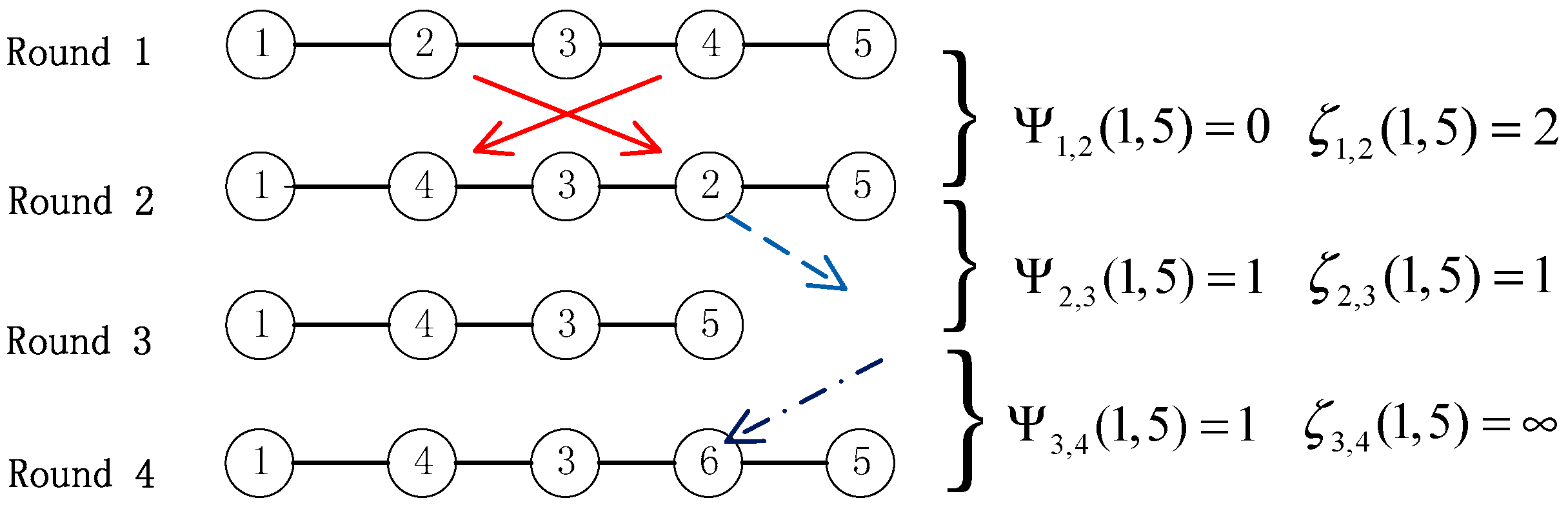
Based on the definition of an instant path, we derive the following notations. Let us denote ρt* as the set of all possible instant paths in Gt, and by ρt*(u, v) those instant paths starting at node u and ending at node v in Gt. The topological length of ρt(u, v) is denoted by |ρt(u, v)| (i.e., the number of hops) and the nodes set of ρt(u, v) is denoted by ||ρt(u, v)||. We denote by (u, v) the order (i.e., position) of node a in ρt(u, v) (if node a is not in ρt(u, v), = ∞), and by the set of nodes which the distance at most d from w in ρt(u, v). For example, if ρt(n1, nk) = <n1, n2, …, nk>, then |ρt(u, v)|=k − 1, ||ρt(n1, nk)||=( n1, n2, …, nk), and , .
To model the dynamicity of instant path, we propose two definitions.
- : the minimum accumulation of node number variance of ρt(u, v) from t to t′ (t′ > t), i.e.,
- : the maximum variance of node order of ρt(u, v) from t to t′ (t′ > t), i.e.,
describes the variance of the node set, i.e., the number of nodes that join in or leave ρt(u, v), while considers the topology variance of nodes in ρt(u, v) due to change of orders. To illustrate the meaning of and , we give example scenarios in Figure 1. In round 2, no nodes leave or join in the path (), and the orders of node 2 and node 4 are varied (). In round 3, the node 2 leaves the path (), and the order of node 5 is varied (). In round 4, the node 6 joins in the path (), and the orders of node 6 and node 5 varied ().
4.2. The (T, l)-Path Model
Now, we model the dynamicity of a network in terms of the variance of the number of nodes and the order of nodes in an instant path. We define a new model named the (T, l)-path.
Definition 3. (T, l)-path:
We say that a dynamic network follows the (T, l)-path model if
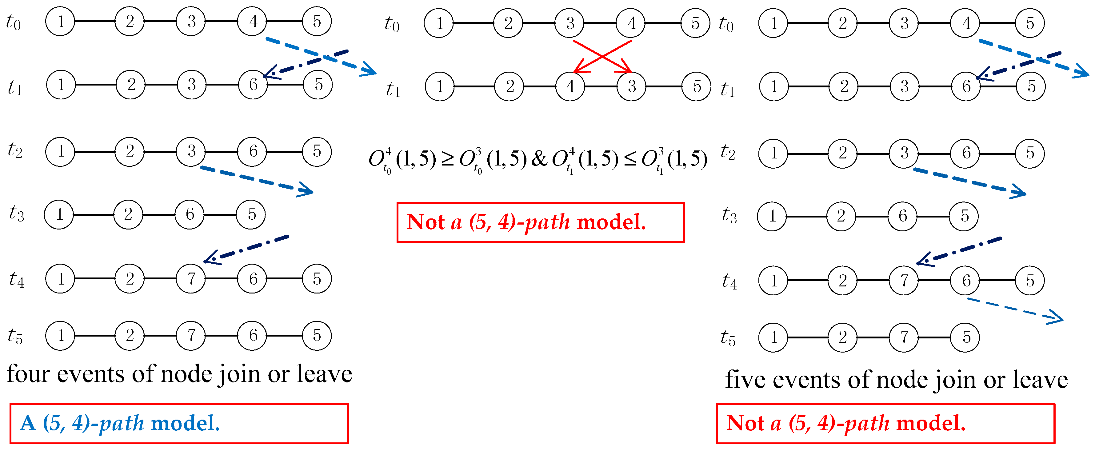
The (T, l)-path model indicates that, for any two nodes u and v, there exists an instant path, and the accumulation variance of the path can be at most l in every T consecutive rounds. That is, there are at most l events of node join and leave in every T consecutive rounds. Please notice that no relative order changes are allowed in the (T, l)-path model. An example illustration of the (T, l)-path model is shown in Figure 2, with T = 5, l = 4. For any node 1 and node 5, there exists an instant path in which there are at most four events of node join in or leaves, in the path in each of the five consecutive rounds. In the same time, the relative order of nodes in such a path cannot change.
Lemma 1.
If a dynamic network follows the (T, l)-path model, for any node u and node v, there exists an instant path ρt(u, v) that follows (T, l)-path and, at most, l nodes can leave or join in such a path every T consecutive rounds.
Proof.
indicates the accumulation of nodes which join in or leave the path. By Definition 3, in every T consecutive rounds. Thus, there are at most l nodes that can leave or join in such a path in every T consecutive rounds. The lemma holds. □
4.3. The (T, l)*-Path Model
The (T, l)-path model allows node leaves or node joins in the path, but pure node order changes are not allowed. Now, we include the node order changes in the dynamicity model, and define the new model as (T, l)*-path as follows.
Definition 4. (T, l)*-path:
We say that a dynamic network follows the (T, l)*-path that:
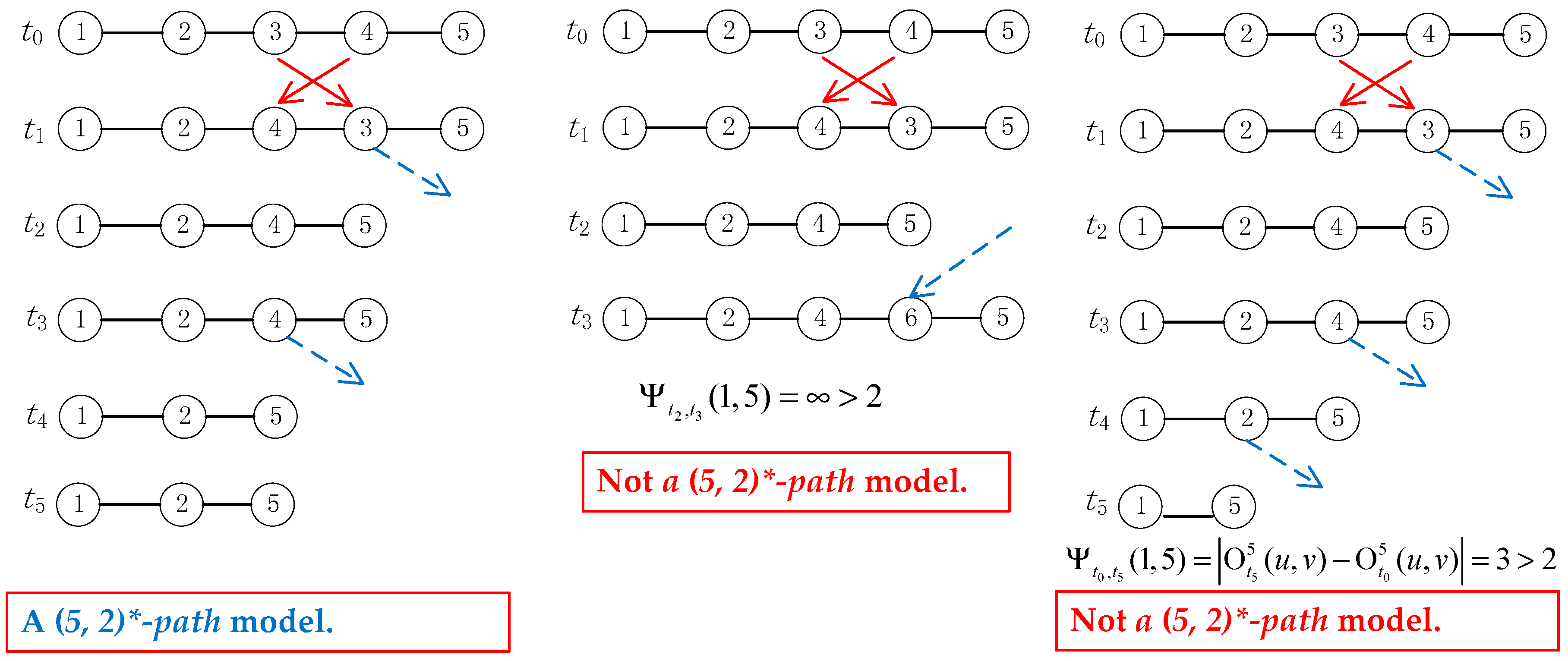
The (T, l)*-path model indicates that, for any two nodes u and v, there exists an instant path that the maximum variance of the node order can be at most l in every T consecutive rounds. An example of the (T, l)*-path model with T = 5, l = 2, is shown in Figure 3. For any node 1 and node 5, there exists an instant path that the maximum variance of the node is at most 2 in every five consecutive rounds.
Lemma 2.
If a dynamic network follows the (T, l)*-path model, for any node u and v, there exists an instant path ρt(u, v) that follows the (T, l)*-path, and at most l nodes can leave such a path every T consecutive rounds.
Proof.
By Definition 4, in every T consecutive rounds. This means that the maximum variance of the node order can be at most l in every T consecutive rounds. If there are more than l nodes leaving the path in every T consecutive round, there is at least one node whose order variance is more than l in T consecutive rounds. This contradicts the definition of the (T, l)*-path model. The lemma holds. □
4.4. The Relationship between the (T, l)-Path and (T, l)*-Path
Both of the two dynamicity models defined above consider the dynamic change of instant path in every T consecutive rounds. The (T, l)-path model focuses on the number of nodes which join in or leave the instant path in every T consecutive rounds, while the (T, l)*-path model concerns the number of nodes leave and the maximum variance of node order.
On the one hand, the (T, l)-path is more general than the (T, l)*-path in terms of node changes in the instant path, i.e., the node joins or leaves the instant path. On the other hand, the (T, l)*-path is more general than the (T, l)-path because it considers node order changes. Therefore, the two models are not equivalent and not comparable.
An interesting question is a model with all possible changes, i.e., node join, leave, and pure order changes. Such a model will be the combination of the (T, l)-path and the (T, l)*-path, and consequently a more general model. We have indeed considered such a model, but it is hard to design an information dissemination algorithm with such a model. The difficulty comes from the complex change scenarios.
4.5. The Relationship between (T, l)-Path and T-Interval Connectivity
The T-interval connectivity model is one of the major connectivity models for dynamic networks. It is interesting to compare our models with the T-interval connectivity model.
Definition 5. T-Interval Connectivity [10]:
We say that a dynamic graph G = (V, E) is T-interval connected for T ≥ 1 if, for all r ∈ N, the static graph is connected.
The underlying meaning of T-interval connectivity is that, for every T consecutive rounds, all the nodes are connected by a spanning subgraph and the subgraph remains unchanged, although topology changes outside the subgraph may occur from round to round.
Two special cases of T-interval connectivity model is 1-interval connectivity and ∞-interval connectivity. With 1-interval connectivity, there is a connected spanning subgraph in each round but the subgraph may change between every two consecutive rounds. A ∞-interval connectivity model requires that there is a connected and static subgraph which does not change all the time.
The T-interval connectivity model is defined in terms of the result of topology changes, while our (T, l)-path and (T, l)*-path models are defined in terms of the procedure of topology changes. Therefore, they cannot be compared directly. That is, we cannot determine which model is more powerful or stronger, or whether one covers the other.
However, connectivity is determined by the procedure of topology changes, i.e., the behaviors of network nodes. From this point of view, our models and the T-internal connectivity model is related to each other. Such a relationship can be reflected by two special cases. In the (T, l)-path model, we can get that, for any node u, node v and t, ρt*(u, v) ≠ Ø, so it belongs to 1-interval connected network.
Similarly, we can get that, the (T, 0)-path and the ∞-interval connectivity are equivalent.
5. The Algorithm for Token Dissemination in (T, l)-Path
Based on the (T, l)-path model, we design two token dissemination algorithms. The first one is for 1-token dissemination and the second one is for k-token dissemination. The correctness of both algorithms is proved.
5.1. Algorithm 1: 1-Token Dissemination in (T, l)-Path
The operations of Algorithm 1 are described below. When the initiator node u wants to disseminate a token c to all the nodes in the network, it will broadcast msg(c, s) in consecutive l + 1 rounds, where s is set to be l + 1 in the first round and decreases one per round. The parameter s indicates the residual number of rounds that node u will broadcast token c. In round i*T + r (i ≥ 0 and r < T), a node v that receives msg(c, s) for the first time will store c, set its s to be m and broadcast msg(c, s) in the following m consecutive rounds, where m is .
Upon receiving msg(c, s) from neighbor nodes in one round, node v chooses the maximum s in msg(c, s), denoted by s′, and the following disseminating operations of v may be changed in two cases. If node v has completed disseminating msg(c, s) and s′ is not smaller than two, v resets its s to be s′-1, and broadcasts msg(c, s) in the following s′-1 consecutive rounds. On the other hand, if node v is broadcasting msg(c, s) in the current round and s′ is greater than s + 2, node v changes its s to be s′-1, and broadcasts msg(c, s) in the following s′-1 consecutive rounds.
Normally, a node stops broadcasting after it conducts the operation for s rounds and terminates the execution of the algorithm. However, as described above, if the node joins a new path it may need to re-start the broadcasting for s rounds. If the node keeps joining new paths, it may not be able to terminate. In such a case, we set n-1 as the upper bound of the number of rounds a node broadcasts the token. That is, a node will terminate broadcasting if it has completed broadcasting in totally n-1 rounds. Such a termination condition is the same as in Reference [10].
| Algorithm 1: 1-token dissemination in the (T, l)-path. |
| Initialization of per node: |
| broNumber ← −1 |
| For nodeu: |
| broNumber ← l + 1 |
| fori = 0, …, l + 1 do |
| broadcasts msg(c, broNumber) |
| broNumber ← broNumber-1 |
| endfor |
| For any nodevin roundi*T + r: |
| ifbroNumber ≠ 0 |
| broadcasts msg(c, broNumbe) |
| broNumber ← broNumber-1 |
| endif |
| receive msg(c, broNumber) from neighbors |
| set TR ← msg(c, broNumber) |
| ifTR is not an empty set |
| set m ← max(broNumber) in TR |
| if broNumber = −1 |
| set broNumber ← |
| endif |
| if broNumber = 0 and m≥2 or broNumber ≤m-2 |
| set broNumber ← m-1 |
| endif |
| endif |
The correctness of Algorithm 1 is proved as below.
Lemma 3 (Termination).
Algorithm 1 can terminate in n-1 rounds, where n is the number of nodes in the network, and the total message size broadcasted in the network is Θ(n2).
Proof.
By Algorithm 1, all the nodes stop broadcasting the message after at most n-1 rounds. Thus, Algorithm 1 can terminate in n-1 rounds. In the worst case, each node will broadcast msg(c, s) in all n-1 rounds and the number of nodes is n. Therefore, the total message size broadcasted in the network is Θ(n2). The lemma holds. □
Theorem 1 (Accuracy).
At the end of Algorithm 1, each node has the token c.
Proof.
For each pair of nodes u and v, there exists at least one instant path that follows Definition 3. We denote this path as ρ(u, v). Then, we only need to prove that node v must receive the token within at most n-1 rounds.
In Algorithm 1, when a node w in ρ(u, v) firstly receives msg(c, s) in round i*T + r (I ≥ 0 and r < T), it will set its s to be m and broadcast msg(c, s) in the following m consecutive rounds, where m is . In such m consecutive rounds, msg(c, s) disseminated along ρ(u, v) and sent by node w may be blocked by the nodes which join in and leave the instant path ρ(u, v). Now, we discuss the impact of the events of node joins and node leaves.
We first consider the scenario that a node z joins in instant path ρ(u, v) and receives msg(c, s) from node w propagated by other nodes in ρ(u, v). According to the operations of Algorithm 1, z must have an s value not smaller than s-1 in msg(c, s) from node w. Therefore, s in msg(c, s) received at z will be decreased by one when the token is further disseminated by node z.
Then, we consider the scenario of node leave. Assuming that a node x, which leaves the instant path ρ(u, v) after receiving msg(c, s) from node w propagated by other nodes in ρ(u, v). We can easily get that, s also decreases by one when it is disseminated through node x.
Combining the case of join and leave, we can get that node join and leave may cause s in msg(c, s) to decrease by one at most. Then, we prove that node w must propagate the token to a node that is nearer to v and propagate the token towards v.
By Lemma 1, the number of nodes which leave the instant path ρ(u, v) is at most l, in every T consecutive rounds. Then, we can get that the number of nodes which leave ρ(u, v) is at most in the round m + i*T + r. Since m is greater than , there exists at least one node y in ρ(u, v) with an order (u, v) > (u, v), and y stays in ρ(u, v) until it receives msg(c, s) propagated from node w (but broadcasted by some other node in ρ(u, v)). If it is the first time that y receives the token, it will act the same as node w: propagating the token in m rounds. Otherwise, if y has ever received the token before it receives the token propagated from w, it must have broadcasted the token for m rounds because it never leaves the path ρ(u, v). In this case, there must exist another node in ρ(u, v) that had received token propagated by y and such a node can further propagate token as w does.
Since purely order change is not allowed (by Definition 3), by simple induction, we can conclude that the token will be propagated towards v one-hop in ρ(u, v) per round, and node v must receive the token finally. Considering is at most n-1, after n-1 rounds, node v must receive msg(c, s). The theorem holds. □
Remark 1.
It is interesting to consider two special scenarios of (T, l)-path: (∞, l)-path and (T, 0)-path. Both these two special models define a quite stable network, where topology changes are not frequent, and Algorithm 1 can be modified under such models, to terminate earlier. In the scenario of (∞, l)-path, when a node v firstly receives token c, it will broadcast c in the following l + 1 consecutive rounds. Each node will terminate once it completes the broadcasting in l + 1 rounds. In the scenario of (T, 0)-path, each node only needs broadcasting c in the next round when it first receives token c. The correctness of such modifications is straightforward and does not need to be presented.
5.2. Algorithm 2: K-Token Dissemination in (T, l)-Path
The Algorithm 2 is for k-token dissemination. Each node needs to maintain three sets. TC is the set of total tokens ever collected. TS is the set of tokens broadcasted by the node. TR is the set of msg(c, s) messages received in each round. Each token is stamped with a unique ID, and this ID is comparable with others.
In each round, a node u broadcasts msg(c, s), where c is not in TS, and it is the minimum in TC, in terms of ID. Each token will be sent in l + 1 consecutive rounds. Node u receives msg(c, s) from its neighbors in the same round and updates its TR and TC. Please notice that TR is emptied at the beginning of each round.
| Algorithm 2:k-token dissemination in the (T, l)-path. |
| Initialization of per node: |
| TC ← |
| TS ← |
| TR ← |
| broNumber ← l + 1 |
| c ← the token c that the node has in the beginning |
| For any nodevin roundi*T + r: |
| ift is not an empty set |
| broadcasts msg(c, broNumbe) |
| broNumber ← broNumber-1 |
| endif |
| receive msg(c′, broNumber) from neighbors |
| TR ← {msg(c′, broNumber)} |
| TA ← {c′} in TR |
| ifTR is not an empty set |
| minID ← minimal ID of token c′ in TR |
| if minID < ID of token c and i<(n-1)* p (the ranks of c′) |
| broNumber ← max(, (n-1)*p-i*T-r) |
| c ← c |
| TS ← TA − {c1, c2,... ci}, which ID of c i is not smaller than minID in TA |
| endif |
| if minID = ID of token c |
| set m ← max(broNumber) in TR |
| if broNumber ≤ m-2 |
| set broNumber ← m-1 |
| endif |
| endif |
| ifbroNumber = 0 |
| set TS=TSc |
| c ← min(TA-TS) |
| broNumber ← l+1 |
| endif |
If the minimum token c′ in TR is smaller than token c and the number of the current round i*T +r (i ≥ 0 and r < T) is smaller than (n-1)*p, where n is the number of the nodes in the network and p is the ranks of token c′ in the descending order in TC, node u will broadcast token c′ instead of token c in the following m consecutive rounds, where m is max(, (n-1)*p-i*T-r). At the same time, node u will delete c′ and tokens not smaller than c′ from TS.
When the minimum token c′ in TR is equal to c, and the maximum value of s in msg(c′, s), denoted by s′, is greater than u′s own s, node u resets its s to be s′-1, and broadcasts msg(c, s) in the following consecutive s′-1 rounds.
After successfully broadcasting token c, node u will add c into TS and start to broadcast the next token.
The correctness of Algorithm 2 is proved as below.
Lemma 4 (Termination).
Algorithm 2 can terminate in (n-1)*k rounds, where n is the number of nodes in the network, and the total message size broadcasted by the algorithm is Θ(n2k).
Proof.
By Algorithm 2, each node will broadcast token 1 once it is received. So each node will obtain token 1 after at most n-1 rounds. Similarly, each node will obtain token 2 after at most 2*(n-1) rounds. Thus, we can easily get that the algorithm can terminate in (n-1)*k rounds.
In the worst case, each node will broadcast tokens throughout all the rounds. Therefore, the total message size broadcasted in the network is Θ(n2k). The lemma holds. □
Theorem 2 (Accuracy).
At the end of Algorithm 2, each node has k tokens.
Proof.
The theorem can be proved by a simple induction. For easy discussion, we denote the k tokens to be disseminated as 1, 2, …, k, respectively. Since token 1 is the minimum token, each node will broadcast it once it is received, as in Algorithm 2. By Lemma 4 and Theorem 1, each node will obtain token 1 after at most n-1 rounds.
When a node u broadcasts token 2, it can only be blocked by the node which is broadcasting token 1. Since token 1 will be finally disseminated successfully, token 2 can be successfully disseminated among all nodes after a finite number of rounds. This can be proved as follows. Without loss of generality, we assume that node u is the last node which broadcasts token 1. After successfully broadcasting token 1, node v will broadcast token 2. Since all the nodes have broadcasted token 1, token 2 becomes the minimum token to be sent and there must not be any node blocked at broadcasting token 2. By Lemma 4 and Theorem 1, each node will have token 2 after at most 2(n-1) rounds.
By simply inducting from token i to token i + 1, we can conclude that, at the end of Algorithm 2, each node will finally have all the k tokens. The theorem holds. □
6. The Algorithm for K-Token Dissemination in (T, L)*-Path
Based on the (T, l)*-path, we design token dissemination algorithms for 1-token and k-token respectively.
6.1. Algorithm 3: 1-Token Dissemination in (T, l)*-Path
Algorithm 3 is for 1-token dissemination. Since there is no node join, the operations of Algorithm 3 are quite straightforward.
When the initiator node u wants to disseminate token c to all the nodes in the network, it will broadcast c in consecutive l + 1 rounds. A node v which receives c for the first time will broadcast c in the following consecutive l + 1 rounds. Each node can terminate once it completes the broadcasting in l + 1 rounds.
| Algorithm 3: 1-token dissemination in the (T, l)*-path. |
| For nodeu: |
| fori = 0, …, l do |
| broadcasts msg(c) |
| endfor |
| For any nodev: |
| if node v receives token c for the first time in round r |
| for i = r+1, …,r+ l + 1 do |
| broadcasts msg(c) |
| endfor |
| endif |
The correctness of Algorithm 3 is proved as below.
Lemma 5 (Termination).
Algorithm 3 can terminate in at most O(n) rounds, where n is the number of nodes in the network, and the total message size broadcasted in the network is Θ(n(l + 1)).
Proof.
By the operations of Algorithm 3, each node broadcasts the token in consecutive l + 1 rounds. Since the number of nodes in the network is n, the algorithm can terminate in O(n) rounds. Correspondingly, the total message size broadcasted in the network is Θ(n(l + 1)). The lemma holds. □
Theorem 3 (Accuracy).
At the end of Algorithm 3, each node has the token c.
Proof.
For any pair of nodes u and v, there exists at least one instant path that follows Definition 4, and we denote such an instant path as ρ(u, v).
If a node x has broadcasted token c for l + 1 consecutive rounds, but its neighbors in ρ(u, v) have not received token c, we mark such a node x as a blocked node. If there is not any blocked node in ρ(u, v), we can easily conclude that node v will receive token c along the path ρ(u, v). The theorem holds in the scenario without blocked nodes.
Now, let us consider the scenario with blocked nodes. We prove the theorem in such a scenario by contradiction. Assume that there is a blocked node in ρ(u, v), which is denoted by w, and w is blocked forever. When node w receives token c for the first time in some round, say r, it will broadcast it in following l + 1 consecutive rounds. Then, any node will receive token c no later than the round r + l + 1, unless node z leaves ρ(u, v). By Definition 4, the maximum variance of node order can be at most l in every T consecutive rounds. Therefore, the neighbors of node w in ρ(r+l+1)(u, v) must have received c. Then node w becomes not blocked, which contradicts the assumption that w is blocked forever. The theorem holds in the scenarios with blocked nodes.
Combining the scenario with and without blocked nodes, the theorem holds. □
6.2. Algorithm 4: K-Token Dissemination in (T, l)*-Path
Algorithm 4 is for k-token dissemination. Each node needs to maintain two sets. TC is the set of total tokens ever collected, and TS is the set of tokens broadcasted by the node. Each token is stamped with a unique ID, and the ID is comparable with others.
In each round, each node u broadcasts token c, where c is not in TS, and it is the minimum in TC in terms of ID. Each token will be sent by a node in l + 1 consecutive rounds. Each node receives tokens from its neighbor nodes at the end of a round and updates its TC. When a token is successfully broadcasted in l + 1 rounds, it will be added into the TS set.
If the minimum token c′ in TC is smaller than c, the token being sent in the current round, c will be replaced by c′ and c′ will be broadcasted in the next consecutive l + 1 rounds. At the same time, all the tokens with an ID greater than c′ will be deleted from TS.
| Algorithm 4:k-token dissemination in the (T, l)*-path. |
| Initialization of per node: |
| TC ← |
| TS ← |
| broNumber ← −1 |
| broID ← MAX |
| For any other nodevin roundi: |
| IDt ← min(TC-TS) |
| if broNumber = −1 or (broNumber ≠ −1 and broID> IDt) |
| broID ← IDt |
| broadcast c to neighbors |
| broNumber ← k |
| TS=TS-{IDj}(which IDj > IDt) |
| endif |
| if broNumber ≠ −1 and broID ≤ IDt |
| broadcast c′ to neighbors (ID of token c′ is broID) |
| broNumber ← broNumber-1 |
| endif |
| if broNumber = 0 |
| set TS=TSbroID |
| broNumber ← −1 |
| borID ← MAX |
| endif |
| receive c1, ..., cs from neighbors |
| TC←TC{c1, ..., cs} |
The correctness of Algorithm 4 is proved as below.
Lemma 6 (Termination).
Algorithm 4 can terminate in at most O(k*n) rounds, where n is the number of nodes in the network, and the total message size broadcasted in the network is Θ(k *n2).
Proof.
By Theorem 3, we need at most n rounds for each token to be disseminated throughout the whole network. Since the number of tokens is k, the time cost is O(k*n) in terms of execution rounds.
In the worst case, each node may broadcast a token in every round. Then, the communication cost is at most Θ(k*n2). The lemma holds. □
Theorem 4 (Accuracy).
At the end of Algorithm 4, each node has all the k tokens.
Proof.
Similarly, the proof is done by induction. we denote the k tokens as the list: 1, 2, …, k. Token 1 is the minimum in a token set, each node receiving token 1 for the first time will broadcast it in the following l + 1 consecutive rounds, and this broadcasting will not be interrupted by other tokens. By Theorem 3, each node will get token 1 at the end of Algorithm 4.
By the (T, l)*-path model, for each pair of nodes u and v, there should be at least one instant path ρ(u, v) with at most l changes in every T consecutive rounds. According to Algorithm 4, node u may broadcast the same token in several series of consecutive rounds. When node u broadcasts token 2 in l+1 consecutive rounds for the last time, it must have successfully broadcasted token 1. By Lemma 5, the neighbors of node u in ρ(u, v) must have broadcasted token 1 when node u broadcasts token 2 for the last time. Then token 2 becomes the minimum in the set of tokens to be sent. When node u broadcasts token 2, its neighbors will also broadcast token 2 in the following l + 1 rounds and this procedure will not be interrupted. Therefore, each node will have token 2 at the end of the algorithm.
By a simple induction, we can conclude that the token will be successfully broadcasted throughout the network, and each node will finally have all the k tokens at the end of Algorithm 4. The theorem holds. □
7. Conclusions and Future Work
In this paper, we study the dynamic network model and the information dissemination algorithm in dynamic networks. Our work includes new model definition, algorithm design, correctness proof, and performance analysis. We first propose the notion of the “instant path” and define two new dynamic network models based on the instant path, i.e., the (T, l)-path and the (T, l)*-path. Differ to the existing dynamic models, the (T, l)-path model focuses on the number of nodes which join in or leave the instant path in every T consecutive rounds, while the (T, l)*-path model concerns the number of nodes that leave and the maximum variance of the node order. We discuss the relationship between our two models and compare them with the T-interval connectivity model. With these two models, we design distributed algorithms for information dissemination respectively, one of the fundamental distributing computing problems. The correctness of all the algorithms is formally proved and their performances in time cost and communication cost are analyzed. To the best of our knowledge, existing algorithms are not suitable for the (T, l)-path model. Thus, the performances cannot be used to compare them against existing algorithms.
Information dissemination in dynamic networks is interesting and challenging. Many efforts should be further made, on both the network model and algorithms. For example, how to improve communication cost by reducing the maximum number of rounds is an interesting topic. Another significant topic is how to choose a desirable path for information dissemination. All existing works guarantee the delivery of tokens by assuming the existence of a path defined by a network model. However, which path is in fact used by tokens is unknown. If we can determine the path used, we can control the dissemination procedure more accurately. Other possible directions include k-token dissemination or counting in the asynchronous network, extending the flat dynamic network models with clusters, etc.
Author Contributions
Conceptualization, Z.Y.; Formal analysis, W.W.
Funding
This research is partially supported by National Key Research and Development Program of China (2016YFB0200400), National Natural Science Foundation of China (No. 61379157, No. 61472455), Program of Science and Technology of Guangdong (No. 2015B010111001), Guangzhou Science and Technology Bureau (201704020030), the Natural Science Foundation of Guangdong Province, China (No. 2016A030310235), and MOE-CMCC Joint Research Fund of China (No. MCM20160104).
Conflicts of Interest
The authors declare no conflicts of interest.
References
- Grindrod, P.; Higham, D.J. Evolving graphs: Dynamical models, inverse problems and propagation. Proc. R. Soc. Lond. Ser. A 2010, 466, 753–770. [Google Scholar] [CrossRef] [Green Version]
- Erlebach, T.; Hoffmann, M.; Kammer, F. On temporal graph exploration. In Proceedings of the International Colloquium on Automata, Languages and Programming, Kyoto, Japan, 6–10 July 2015; pp. 444–455. [Google Scholar]
- Datta, S.; Giannella, C.; Kargupta, H. K-means clustering over a large, dynamic network. In Proceedings of the Sixth SIAM International Conference on Data Mining, Bethesda, MD, USA, 20–22 April 2006; pp. 153–164. [Google Scholar]
- Vaidya, N.H.; Krishna, P.; Chatterjee, M.; Pradhan, D.K. A Cluster-based approach for routing in dynamic networks. ACM SIGCOMM Comput. Commun. Rev. 1997, 27, 49–64. [Google Scholar]
- Michail, O.; Chatzigiannakis, I.; Spirakis, P.G. Naming and counting in anonymous unknown dynamic networks. In Proceedings of the 26th International Symposium on Distributed Computing (DISC), Salvador, Brazil, 16–18 October 2012; pp. 437–438. [Google Scholar]
- Kuhn, F.; Oshman, R. Dynamic networks: Models and algorithms. ACM SIGACT News 2011, 42, 82–96. [Google Scholar] [CrossRef]
- Van de Bovenkamp, R.; kuipers, F.; van Mieghem, P. Gossip-based counting in dynamic networks. In Proceedings of the 11th International IFIP TC 6 Networking Conference, Prague, Czech Republic, 21–25 May 2012; pp. 404–417. [Google Scholar]
- O’Dell, R.; Wattenhofer, R. Information dissemination in highly dynamic graphs. In Proceedings of the 9th Joint Workshop on Foundations of Mobile Computing, Cologne, Germany, 2 September 2005; pp. 104–110. [Google Scholar]
- Haeupler, B.; Karger, D. Faster information dissemination in dynamic networks via network coding. In Proceedings of the ACM SIGACT-SIGOPS Symposium on Principles of Distributed Computing, San Jose, CA, USA, 6–8 June 2011; pp. 381–390. [Google Scholar]
- Kuhn, F.; Lynch, N.; Oshman, R. Distributed computation in dynamic networks. In Proceedings of the 42nd ACM Symposium on Theory of Computing, Cambridge, MA, USA, 6–8 June 2010; pp. 513–522. [Google Scholar]
- Kempe, D.; Kleinberg, J.; Kumar, A. Connectivity and inference problems for temporal networks. In Proceedings of the 32nd Annual ACM Symposium on Theory of Computing (STOC), Portland, OR, USA, 21–23 May 2000; pp. 504–513. [Google Scholar]
- Casteigts, A.; Flocchini, P.; Quattrociocchi, W.; Santoro, N. Time-Varying graphs and dynamic networks. Int. J. Parallel Emerg. Distrib. Syst. 2012, 27, 387–408. [Google Scholar] [CrossRef]
- Shang, Y. Multi-agent coordination in directed moving neighbourhood random networks. Chin. Phys. B 2010, 19, 070201. [Google Scholar] [Green Version]
- Shang, Y. Consensus in averager-copier-voter networks of moving dynamical agents. Chaos Interdisciplin. J. Nonlinear Sci. 2017, 27, 215–233. [Google Scholar] [CrossRef] [PubMed]
- Clementi, A.; Macci, C.; Monti, A.; Pasquale, F.; Silvestri, R. Flooding time in edge-markovian dynamic graphs. In Proceedings of the 27th ACM Symposium on Principles of Distributed Computing, Toronto, ON, Canada, 18–21 August 2008; pp. 213–222. [Google Scholar]
- Avin, C.; Koucky, M.; Lotker, Z. How to explore a fast-changing world (cover time of a simple random walk on evolving graphs). In Proceedings of the 35th International Colloquium on Automata, Languages and Programming, Reykjavik, Iceland, 7–11 July 2008; pp. 121–132. [Google Scholar]
- Pittel, B. On spreading a rumor. SIAM J. Appl. Math. 1987, 47, 213–223. [Google Scholar] [CrossRef]
- Clementi, A.; Monti, A.; Silvestri, R. Flooding over Manhattan. In Proceedings of the 29th ACM Symposium on Principles of Distributed Computing, Zurich, Switzerland, 25–28 July 2010. [Google Scholar]
- Shang, Y. The Estrada index of evolving graphs. Appl. Math. Comput. 2015, 250, 415–423. [Google Scholar] [CrossRef]
- Shang, Y. Laplacian Estrada and normalized Laplacian Estrada indices of evolving graphs. PLoS ONE 2015, 10, e0123426. [Google Scholar] [CrossRef] [PubMed]
- Wehmuth, K.; Fleury, E.; Ziviani, A. On multiaspect graphs. Theor. Comput. Sci. 2016, 651, 50–61. [Google Scholar] [CrossRef]
- Ahmadi, M.; Ghodselahi, A.; Kuhn, F.; Molla, A.R. The cost of global broadcast in dynamic radio networks. In Proceedings of the International Conference on Principles of Distributed Systems, Rennes, France, 14–17 December 2015. [Google Scholar]
- Yang, Z.; Wu, W.; Chen, Y.; Li, X.; Cao, J. (Q, S)-distance model and counting algorithms in dynamic distributed systems. Int. J. Distrib. Sens. Netw. 2018, 14. [Google Scholar] [CrossRef]
- Jelasity, M.; Guerraoui, R.; Kermarrec, A.; Steem, M. The peer sampling service: Experimental evaluation of unstructured gossip-based implementations. In Proceedings of the 5th ACM/IFIP/USENIX International Conference on Middleware, Toronto, ON, Canada, 18–22 October 2004; pp. 79–98. [Google Scholar]
- Clementi, A.; Crescenzi, P.; Doerr, C.; Fraigniaud, P.; Pasquale, F.; Silvestri, R. Rumor spreading in random evolving graphs. Random Struct. Algorithms 2016, 48, 290–312. [Google Scholar] [CrossRef]
- Acan, H.; Collevecchio, A.; Mehrabian, A.; Wormald, N. On the push & pull protocol for rumor spreading. SIAM J. Discret. Math. 2017, 31, 647–668. [Google Scholar]
- Augustine, J.; Chen, A.; Liaee, M.; Pandurangan, G.; Rajaraman, R. Information spreading in dynamic networks under oblivious adversaries. In Proceedings of the International Symposium on Distributed Computing, Paris, France, 27–29 September 2016; pp. 399–413. [Google Scholar]
Figure 1.
An examples of the instant path dynamicity.

Figure 2.
An example illustration of a (5, 4)-path model.

Figure 3.
An example of a (5, 2)*-path model.

© 2018 by the authors. Licensee MDPI, Basel, Switzerland. This article is an open access article distributed under the terms and conditions of the Creative Commons Attribution (CC BY) license (http://creativecommons.org/licenses/by/4.0/).
Share and Cite
MDPI and ACS Style
Yang, Z.; Wu, W. The (T, L)-Path Model and Algorithms for Information Dissemination in Dynamic Networks. Information 2018, 9, 212. https://0-doi-org.brum.beds.ac.uk/10.3390/info9090212
AMA Style
Yang Z, Wu W. The (T, L)-Path Model and Algorithms for Information Dissemination in Dynamic Networks. Information. 2018; 9(9):212. https://0-doi-org.brum.beds.ac.uk/10.3390/info9090212
Chicago/Turabian StyleYang, Zhiwei, and Weigang Wu. 2018. "The (T, L)-Path Model and Algorithms for Information Dissemination in Dynamic Networks" Information 9, no. 9: 212. https://0-doi-org.brum.beds.ac.uk/10.3390/info9090212
Note that from the first issue of 2016, this journal uses article numbers instead of page numbers. See further details here.