The CLoTH Simulator for HTLC Payment Networks with Introductory Lightning Network Performance Results

Abstract

The Lightning Network (LN) is one of the most promising off-chain scaling solutions for Bitcoin, as it enables off-chain payments which are not subject to the well-known blockchain scalability limit. In this work, we introduce CLoTH, a simulator for HTLC payment networks (of which LN is the best working example). It simulates input-defined payments on an input-defined HTLC network and produces performance measures in terms of payment-related statistics (such as time to complete payments and probability of payment failure). CLoTH helps to predict issues and obstacles that might emerge in the development stages of an HTLC payment network and to estimate the effects of an optimisation action before deploying it. We conducted simulations on a recent snapshot of the HTLC payment network of LN. These simulations allowed us to identify network and payments configurations for which a payment is more likely to fail than to succeed. We proposed viable solutions to avoid such configurations.

1. Introduction

Bitcoin is a decentralised cryptocurrency that allows mistrusting peers to send/receive monetary value without the need for intermediaries [1]. Bitcoin relies on the blockchain, a distributed peer-to-peer public ledger where each peer stores all the history of Bitcoin economic transactions. Its distributed and replicated nature along with a limited block dimension entails capped transaction throughput [2]. As proven in the comprehensive study by Gervais et al. [3], although more recent blockchains introduced technical solutions to reduce its extent, a commonly accepted blockchain design that resolves the scalability issue is not yet known.

One of the more explored technical proposals that addresses the blockchain scalability issue is the off-chain scaling [4,5,6,7,8,9,10], which enables off-chain payments, i.e., payments that do not need to be registered on the blockchain. Off-chain scaling approaches are based on payment channels. A payment channel is a two-party ledger which is updated off-chain and uses the underlying blockchain only as a settlement or dispute resolution layer. It allows an unbounded number of off-chain payments to be sent/received between two involved parties (the channel endpoints), as long as they can jointly reach consensus.

Two-party payment channels can be linked together to build a payment network for off-chain payments. This allows parties not directly connected by a payment channel to send/receive off-chain payments which are routed across a network of linked payment channels.

The Lightning Network (LN) [4] is the most developed off-chain solution and the mainstream payment network for Bitcoin. The LN protocol leverages a particular contract called Hashed Timelock Contract (HTLC) to build the payment network. The HTLC scheme allows transferring off-chain payments through multiple payment channels linked together. It guarantees transfer atomicity: even if a payment is carried across multiple intermediate channels to reach the recipient, the payment either succeeds or fails in all the involved channels. Henceforth, we define the HTLC payment network as a network of linked payment channels where payments are transferred using the HTLC scheme.

At its current state of development, the LN protocol is characterised by features that, if not properly understood, implemented and controlled, might undermine the development of a healthy HTLC payment network, i.e., a network that supports fast and successful payments. The features that need to be studied are the following: (1) source routing, i.e., a good routing path that does not cause a payment failure depends on the knowledge of an up-to-date network topology; (2) channel capacity, which constrains the payment amount; (3) channel unbalancing, namely, the condition of a skewed channel that has one endpoint depleted due to a number of unidirectional payments (an issue not internally addressed by the LN protocol); and (4) uncooperative behaviour of peers involved in a payment route, which increases payment time.

To avoid that these factors prevent the correct functioning of the HTLC payment network, also one of the more accredited LN development group claims the importance of protocol improvements and optimisation actions: in particular, the developers envision the need for special routing nodes, which are always online and contribute enough capital to route payments [11]. However, since the LN protocol design aims at ensuring systemic censorship resistance, the resulting lack of central coordination does not allow to predict outcomes of specific network configurations and/or optimisations.

In this work we present CLoTH, an HTLC payment network simulator. CLoTH simulator is a tool: to predict issues and obstacles that might emerge in development stages of an HTLC payment network; to assist in planning uncoordinated development of the network; to estimate the effects of an optimisation action before deploying it; to predict the return on investment of adding a hub to the network.

Examples of questions (expressed in simple English words) that can be answered by CLoTH are: (1) “How many channels per peer are required to have a robustly connected network?”; (2) “Which is the impact on performances of peers going offline?”; (3) “In which way payment amounts influence the probability of payment failures?”; (4) “How the mean payment time decreases by adding a peer with a specific set of payment channels in a specific point of the network?”.

The main contributions of our research are:

• The CLoTH simulator. It is a discrete-event simulator that simulates payments on HTLC payment networks. It takes as input parameters defining an HTLC network (e.g., number of peers and number of channels per peer) and parameters of the payments to be simulated on the defined HTLC network (e.g., the payment rate and payment amounts). It generates performance measures in the form of payment statistics, e.g., the probability of payment failure and the mean payment complete time. To the best of our knowledge, CLoTH is the first available simulator of HTLC payment networks.
• Simulation results produced using a recent snapshot of the HTLC payment network of LN. Such simulations allowed us to discover interesting cases when a payment is more likely to fail than to succeed on such network. Two such cases are the following: (1) when we set the payment rate to 100 payments per second, the network experienced 56.12% probability of payment failure; and (2) when we simulated payment amounts whose order of magnitude is between 1 millisatoshi and 0.0001 BTC (being worth less than $1 at the time of writing), the network experienced 53.87% probability of payment failure.

Other contributions of our research are additional simulation runs on synthetic HTLC networks (i.e., HTLC payment networks generated by the simulator using their statistical description). The results of these simulations show that: almost all synthetic networks have good performance (nearly 99% probability of payment success); if a network has 100 thousands peers, at least five channels per peers are required to have a well-connected decentralised network.

The remainder of the paper is organised as follows. Section 2 is a background on Bitcoin, off-chain scaling solutions and the Lightning Network. In Section 3, we describe the LN code we used as reference to develop the simulator. In Section 4, we present in detail the CLoTH simulator. In Section 5, we explain the design of the simulations we conducted. In Section 6, we show and discuss the results of the simulations. Finally, in Section 7, we provide conclusions and some possible future work.

2. Background

In this Section, we briefly explain the main concepts constituting the background of our research: Bitcoin and the blockchain; off-chain scaling solutions; and the Lightning Network.

2.1. Bitcoin and the Blockchain

Bitcoin is a decentralised payment system running on a peer-to-peer network. Transactions are used to transfer bitcoin cryptocurrency and they are defined by an input state and an output state. The output is represented by the amount of currency to be transferred and by a Bitcoin script defining the spending conditions to claim that amount. The input is represented by the reference to an output of a previous transaction and the proof fulfilling the spending conditions of the referenced output. The blockchain is the distributed ledger technology storing all Bitcoin transactions. Each peer (that runs a full node) stores a whole copy of the ledger. Miners are special peers that can write on the ledger: (i) they validate transactions broadcast on the peer-to-peer network against the ledger in order to prevent double spending of coins; and (ii) they gather transactions and write on the ledger, by broadcasting a block (i.e., a collection of transactions), ideally once every 10 min. For more details on Bitcoin and the blockchain, we refer the reader to the detailed background study by Bonneau et al. [12].

The Bitcoin blockchain is affected by a well-known scalability problem. Each block, in fact, has bounded size which imposes a limit to the transaction throughput. Such limit, on the one hand, contains the cost of storing the blockchain and validating and transmitting transactions [13], but, on the other hand, with a block size limit of 1 MB, the maximum transaction throughput is capped at around only seven transactions per second [14].

2.2. Off-Chain Scaling Approaches

Off-chain scaling approaches pursuit scalability by moving off-blockchain as many transactions as possible.

2.2.1. Payment Channels

Payment channels [15] are the building block of the off-chain protocols. Such channels are implemented as two-party ledgers that allow two parties (the channel endpoints) to update their balances off-chain, without the limit imposed to blockchain transactions. The blockchain is used only as a dispute resolution layer when and if consensus about the off-chain state cannot be reached off-chain between channel endpoints.

In the rest of this section, we leverage the following example of a payment channel.

Payment channel example. Alice and Berto open a payment channel. Alice funds the channel with 0.5 BTC, Berto funds the channel with 0.5 BTC, so Alice’s initial balance in the channel is 0.5 BTC and Berto’s is 0.5 BTC. The capacity of the channel is the total amount of bitcoins in the channels: 1 BTC. After opening the channel, Alice can transfer 0.1 BTC off-chain to Berto: to do so, they update accordingly their balances in the channel, thus Alice’s balance is 0.4 BTC and Berto’s balance is 0.6 BTC. Channels are bidirectional, so also Berto can pay Alice. It is important to notice that no transactions on the blockchain are required to accomplish these payments between Alice and Berto: they just update their bidirectional off-chain balances.

2.2.2. Payment Network

A payment network is a network of payment channels linked together, to avoid that every possible pair of peers has to open bidirectional payment channels for off-chain payments. With respect to blockchain transactions, off-chain payments performed in payment networks are: cheaper, as lower fees are required to route payments in such networks; faster, as they do not need to be registered on the blockchain; and more privacy preserving, as they are not visible in the public blockchain.

In the rest of the section, we leverage the following example of a payment network.

Payment network example. Alice sends 0.1 BTC off-chain to Davide, without having a direct payment channel with him. She exploits a route of already open channels linking her to Davide: the channel she has with Berto; the channel between Berto and Carola; and the channel between Carola and Davide. To find this route of payment channels, source routing is applied: it is Alice who has to find which intermediary hops her payment needs to go through.

2.3. The Lightning Network

The Lightning Network (LN) is the mainstream implementation of a network of payment channels for Bitcoin. It was introduced in 2015 by Joseph Poon and Thaddeus Dryja [4].

2.3.1. LN Payment Channel Lifecycle

The payment channel lifecycle, as specified by the LN protocol, is presented in the following.

Channel funding. Alice and Berto create a funding transaction, the transaction required to fund the channel. The funding transaction is broadcast to the blockchain and, when confirmed, the channel is considered open. Alice and Berto create also a commitment transaction, which represents their respective current balances in the channel: such transaction spends the bitcoins in the funding transaction and transfers 0.5 BTC to Alice and 0.5 BTC to Berto. The commitment transaction is not broadcast to the blockchain.

Payment execution. When Alice wants to pay 0.1 BTC to Berto, the two parties create a new commitment transaction which reflects the new balances: 0.4 BTC of Alice and 0.6 BTC of Berto. No transaction is sent to the blockchain, i.e., the operation is done off-chain.

Channel closing. When the two parties want to close the channel, they send the last updated commitment transaction to the blockchain.

Punishments to disincentivise misbehavior. Berto can punish Alice if Alice misbehaves (or vice versa), thanks to the Revocable Sequence Maturity Contract (RSMC), a contract implemented by a script in the spending condition of the commitment transaction. Alice could be tempted to broadcast an old commitment to the blockchain, for instance, the commitment preceding her payment to Berto, when she owned more funds (0.5 against 0.4 BTC). If Alice tries to do so and Berto notices the old commitment transaction in the blockchain, Berto can take all the funds of the channel (even the 0.4 BTC of Alice’s balance), by broadcasting the last commitment transaction with the RSMC to the blockchain. Therefore, since Alice may lose all her funds, she is disincentivised to misbehave.

Channel unbalancing. A channel is said unbalanced or skewed when one balance is much higher than the other. If payments always flow from Alice to Berto and no payments flow from Berto to Alice, Alice’s balance may go to zero. Channel unbalancing constitutes a problem, as a payment cannot traverse a channel in a given direction if the balance in that direction is lower than the payment amount.

2.3.2. Hashed Timelock Contract (HTLC)

HTLC is a contract for off-chain multi-hop payment through channels that connect the payment sender and the payment recipient. An off-chain multi-hop payment is the atomic composition of several off-chain payments, each one performed on an intermediate payment channel. An intermediate peer receives an inbound payment on one of its channels and forwards the same amount to the next payment hop (actually a little less since it retains a small fee for intermediary service), until the payment arrives to the recipient. In this way, the HTLC scheme creates a network of payment channels along which off-chain payments can be routed.

In practice, the HTLC contract is implemented by a script in the spending condition of the commitment transaction of a payment channel and it executes conditional payments. Alice pays 0.1 BTC to Berto if Berto can demonstrate to know a value R within a certain timeout (timelock, in the Bitcoin jargon): in this case, the HTLC is fulfilled; otherwise, 0.1 BTC returns back to Alice and the HTLC fails. Funds in the HTLC payment stay locked up to the disclosure of R or, if R is never disclosed, up to the timelock expiration. In the following, we describe the phases of a payment from Alice to Davide using HTLCs.

HTLC establishment. For the multi-hop payment originated by Alice and trying to reach Davide, the following HTLCs are established: (1) the HTLC between Alice and Berto, where Alice pays 0.1 BTC to Berto if Berto demonstrates to know R within a certain timelock, e.g., three days; (2) the HTLC between Berto and Carola, where Berto pays 0.1 BTC to Carola if Carola demonstrates to know R within two days; and (3) the HTLC between Carola and Davide, where Carola pays 0.1 BTC to Davide if Davide demonstrates to know R within one day.

HTLC fulfillment. Alice sends R to Davide, and HTLCs from Davide to Alice are fulfilled: Davide shows R to Carola within one day, and Carola pays him 0.1 BTC; Carola shows R to Berto within two days, and Berto pays her 0.1 BTC; Berto shows R to Alice within three days, and Alice pays him 0.1 BTC. At the end, 0.1 BTC has been transferred from Alice to Davide. For their work of forwarding the payment, Berto and Carola can withhold a small fee when transferring the payment (which, for simplicity, we omitted in this example). It is important to highlight that all the described operations are performed off-chain, without the need to interact with the blockchain. Finally, it is worth noticing that, from Davide to Alice, HTLCs have increasing timelocks. This ensures that each party has enough time to know R and claim her funds: Davide shows R to Carola in one day, Carola pays 0.1 BTC to Davide; after that, Carola still has one day to claim 0.1 BTC from Berto, as the timelock with Berto is set to two days.

HTLC failure. If R is not disclosed by an uncooperative peer, the payment fails in all channels. A failure message is sent back to Alice and no payment occurs between the channels, as HTLC conditions have not been fulfilled. In addition, in such case, funds in the HTLC stay locked up to the timelock expiration. If Davide does not disclose R, Carola has to wait one day to get back 0.1 BTC according to the HTLC conditions. After that, Carola closes the channel with Davide by broadcasting the last commitment transaction to the blockchain and propagates back the failure to Alice.

2.4. Brief Literature

Although the most developed, the Lightning Network is not the only off-chain payment network in the literature.

Christian Decker presented Duplex Micropayment Channels for building an off-chain payment network based on HTLCs [5]. With respect to this approach, the key novelty of LN is the possibility of punishing a misbehaving party in the channel.

Raiden [7] uses smart contracts to implement the same fundamental concepts of LN in the Ethereum blockchain.

Sprites [6] is an attempt to improve both LN and Raiden, as it aims at minimising the time during which funds are locked while being transferred via HTLCs.

3. Preliminary Analysis

For implementation level details of HTLC mechanisms, we took as reference lnd, the Golang implementation of the Lightning Network. lnd, as the other LN implementations (e.g., c-lightning [16], and eclair [17]), fully conforms to the so-called Basis of Lightning Technology (BOLT) [18], the Lightning Network specifications.

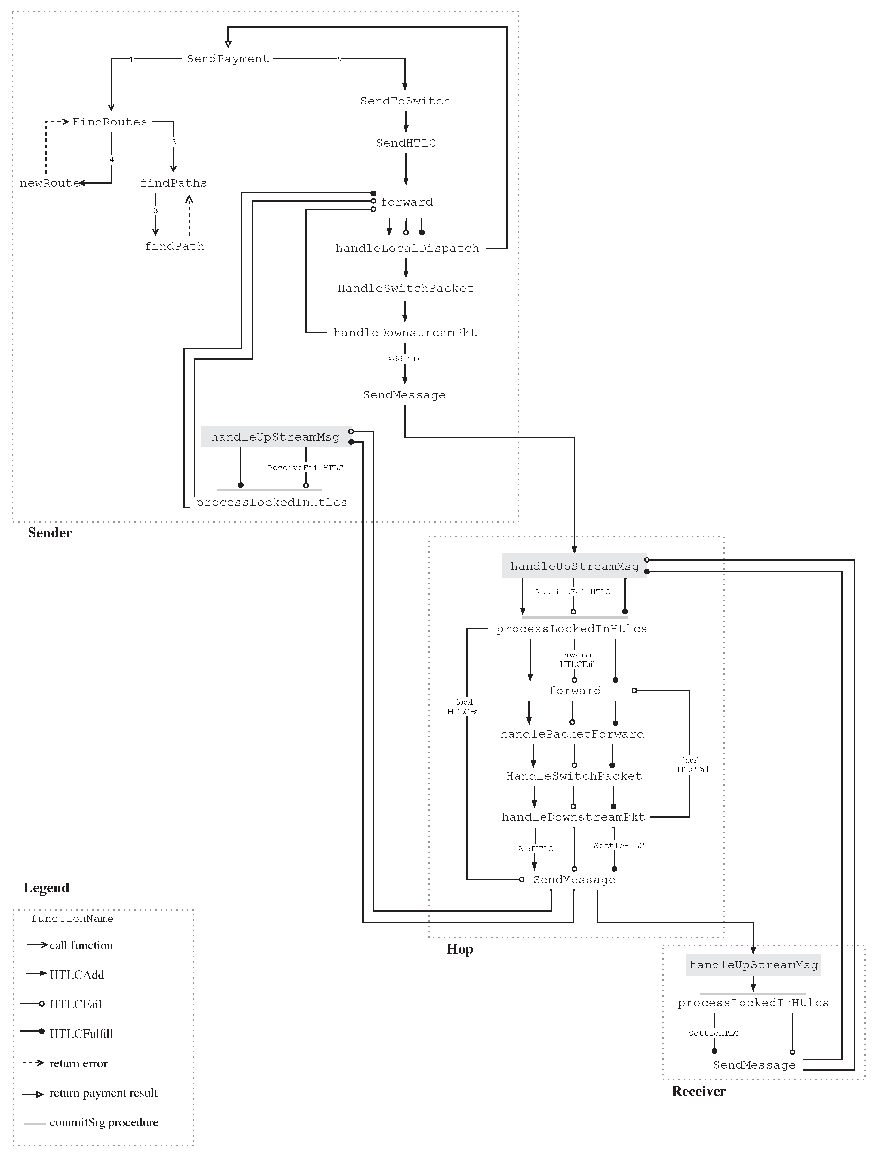
In Figure 1, we show the multi-hop payment call graph resulting from our analysis of commit 65dede2 of the lnd public GitHub repository (while for our implementation we used commit 4d6cd2e, a more recent commit in which function findPaths has been replaced by a blacklist-based routing described below). The call graph represents the functions called when a payment flows from a sender to a receiver through an intermediate hop. These functions implement the HTLC mechanism that ensures the atomicity of the payment (cf. Section 2.3.2).

We depict three peers, as they call different functions with different behaviours: the payment sender $\mathcal{S}$, the payment receiver ℜ and a generic intermediate hop ℌ. This case can be easily generalised to the n-intermediaries one since the behaviour of each intermediate hop is always the same.

HTLC messages (i.e., HTLCAdd, HTLCFulfill and HTLCFail) that flow through peers are represented by arrows:

• HTLCAdd: sent from $\mathcal{S}$ to ℜthrough ℌ, for the establishment of HTLCs among the peers;
• HTLCFulfill: sent from ℜ to $\mathcal{S}$ through ℌ, for the fulfillment of the HTLCs; and
• HTLCFail: sent in case of failures, for failing the HTLCs.

The function handleUpStreamMsg in the gray box represents the first function called by a peer when an HTLC message is received. The gray line represents the commitSig procedure that establishes an HTLC: the creation of a new commitment transaction containing the HTLC between the two involved parties.

In Appendix A, we describe the details of the lnd code and of the functions of the call graph, while in the following we provide an high-level description of the flow of a payment.

Payment initialisation and sending. Source routing is run by $\mathcal{S}$ to search for an available route to ℜ. If no route is found, the payment is considered failed; otherwise, $\mathcal{S}$ sends an HTLCAdd message to ℌ to establish the HTLC.

Payment relay (intermediate hop). ℌ checks for possible errors (e.g., it checks whether it has enough balance to forward the payment). If there are errors, it sends an HTLCFail message back to $\mathcal{S}$, failing the HTLC; otherwise, it sends an HTLCAdd message to ℜ. (This step occurs multiple times in the general case of a payment going through multiple intermediate hops.)

Payment reception. ℜ checks for possible errors. If there are errors, it sends an HTLCFail message to ℌ (which in turn propagates it to $\mathcal{S}$), failing the HTLCs; otherwise, it sends an HLTCFulfill message to ℌ (which in turn propagates it to $\mathcal{S}$), for fulfilling the HTLCs.

Payment re-attempt. If an HTLCFail is received by $\mathcal{S}$, $\mathcal{S}$ tries to re-attempt the payment by searching for a new route. If the failure was due to a channel which did not have enough balance to forward the payment, the channel is blacklisted. If the failure, instead, was due to an uncooperative peer, the peer is blacklisted. A new route is looked for excluding peers and channels in the blacklist. If no new route is found, the payment is considered definitively failed.

4. Simulator Design

In this Section, we provide a detailed description of the CLoTH simulator, which is, to the best of our knowledge, the first simulator for HTLC payment networks. By HTLC payment network, we mean a network where peers are connected by payment channels and off-chain payments are routed using HTLC contracts.

The simulator takes as input the definition of an HTLC network and the payment script to be played during the simulation. It simulates payments in the HTLC network by locally running a discrete-event mapping of the lnd code. It produces performance measures in the form of payment-related statistics (e.g., the probability of payment failures and the mean payment complete time).

4.1. Assumptions

An HTLC payment network relies on a blockchain as a securing mechanism for all the payment channels which form the network. The underlying blockchain is therefore a fundamental prerequisite of each HTLC payment network. We assume channels are loaded with an amount of native tokens from the underlying blockchain and fees for payment forwarding are due to the intermediary hops in the same denomination.

CLoTH does not consider blockchain interactions during a simulation execution, since the performance measures produced by the simulator are related to payments, which are completely performed off-chain. Simulations run on a network in which no new channels are opened. This condition is implicitly guaranteed if the whole simulation time is shorter than the time required to accumulate a large enough number of confirmations for funding a new channel with an on-chain transaction. For this reason, we made each simulation last about 15 min, since to deem a transaction as definitive on Bitcoin it is usual to wait for six confirmations (about 60 min). Without loss of generality, we do not take into account those channels that might have been established early enough before the simulation starting time to become operative during the simulation time window.

Another assumption we made in the simulator is that each peer has a complete and precise knowledge of all other peers and channels in the network. In reality, as specified in BOLT, new channels and peers are announced through a gossip protocol. Therefore, real performance may result slightly worse than the one measured by CLoTH, as in reality peers may have a slightly imprecise knowledge of the network, due to imperfections of the gossip protocol.

4.2. Software Architecture

CLoTH is a discrete-event simulator [19]. Events represent state changes of the simulated system. The event loop is the core of the simulation engine: it extracts the next event from a queue where events are sorted according to their occurring time; it advances the simulation time to the instant of occurrence of the event being currently processed; and it calls the function that processes the event.

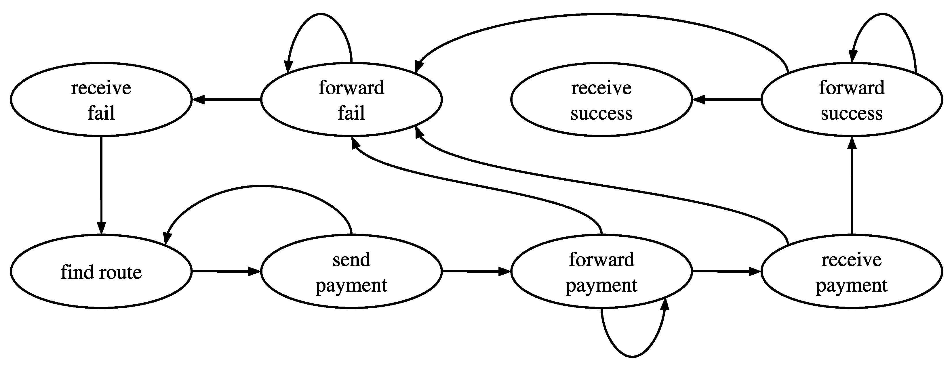
The simulator generates an event each time a payment changes its state according to the state diagram in Figure 2. Each type of event in the diagram is processed by a function of the same name of the simulator, as explained in the following Section.

4.2.1. Computation Flow

Table 1. Mapping between CLoTH simulator functions and lnd functions.

Simulator Function	Description	Simulated Functions	Peer	Message
find_route	Search for a payment route	SendPayment, FindRoutes, findPath, newRoute	Sender	-
send_payment	Send a payment	SendToSwitch, SendHTLC, forward, handleLocalDispatch, HandleSwitchPacket, handleDownstreamPkt, AddHTLC, SendMessage	Sender	HTLCAdd
forward_payment	Forward a payment	handleUpstreamMsg, processLockedInHtlcs, forward, handlePacketForward, HandleSwitchPacket, handleDownstreamPkt, AddHTLC, SendMessage	Hop	HTLCAdd
receive_payment	Receive a payment	handleUpstreamMsg, processLockedInHtlcs, SendMessage, SettleHTLC	Receiver	HTLCAdd
forward_success	Forward the successful result of a payment	handleUpstreamMsg, processLockedInHtlcs, forward, handlePacketForward, HandleSwitchPacket, handleDownstreamPkt, SettleHTLC, SendMessage	Hop	HTLCFulfill
forward_fail	Forward the fail result of a payment	handleUpstreamMsg, processLockedInHtlcs, forward, handlePacketForward, HandleSwitchPacket, handleDownstreamPkt, ReceiveFailHTLC, SendMessage	Hop	HTLCFail
receive_success	Receive the successful result of a payment	handleUpstreamMsg, processLockedInHtlcs, forward, handleLocalDispatch	Sender	HTLCFulfill
receive_fail	Receive the fail result of a payment	handleUpstreamMsg, processLockedInHtlcs, forward, handleLocalDispatch, ReceiveFailHTLC	Sender	HTLCFail

shows the mapping between each function of the lnd computation flow and functions of the CLoTH simulator codebase. The completeness of the mapping ensures the validity of the simulated results.

Table 1 makes a clear distinction between particular behaviours of each lnd function which depends on two parameters: (1) the type of peer that invokes it (i.e., sender, receiver or intermediate hop); and (2) the type of the triggering message (HTLCAdd, HTLCFail, HTLCFulfill). For example, the function send_payment of the simulator simulates the functions SendToSwitch, SendHTLC, forward, handleLocalDispatch, HandleSwitchPacket, handleDownstreamPkt, AddHTLC and SendMessage of the lnd code, when they are called by the payment sender in the case of HTLCAdd message.

Uncooperative behaviour. Functions forward_payment, receive_payment and forward_success simulate the uncooperative behaviour of a peer. Using Bernoulli probability distributions, we determine whether a peer is uncooperative and, if so, whether it is uncooperative after or before establishing the HTLC. If the peer is cooperative, the function is normally executed. If the peer is uncooperative before establishing the HTLC, as specified by the LN protocol, an HTLCFail is propagated back to the payment sender and the payment is re-attempted with a new route that does not encompass the uncooperative peer. Finally, if the peer is uncooperative after establishing the HTLC, as specified by the LN protocol, an HTLCFail is propagated back to the payment sender after the timelock expiration and the channel connecting to the uncooperative peer is closed. Then, the sender can re-attempt the payment, with a new route excluding the closed channel.

4.2.2. Data Structures

Figure 3 shows main attributes of the simulator data structures. A channel connects two peer (each one represented by an ID) and has a certain capacity. The endpoint of a channel describes how a peer behaves in a specific channel and contains: the current balance of the endpoint in that channel; base and proportional fee, which constitute the fee withheld by the endpoint for forwarding a payment (proportional fee is the part of the fee which depends on the payment amount, while base fee is the constant fee applied regardless of the payment amount); and the timelock set in the HTLCs established by the channel endpoint. A payment is described by a sender, a receiver and the payment amount.

4.3. Workflow and Usability

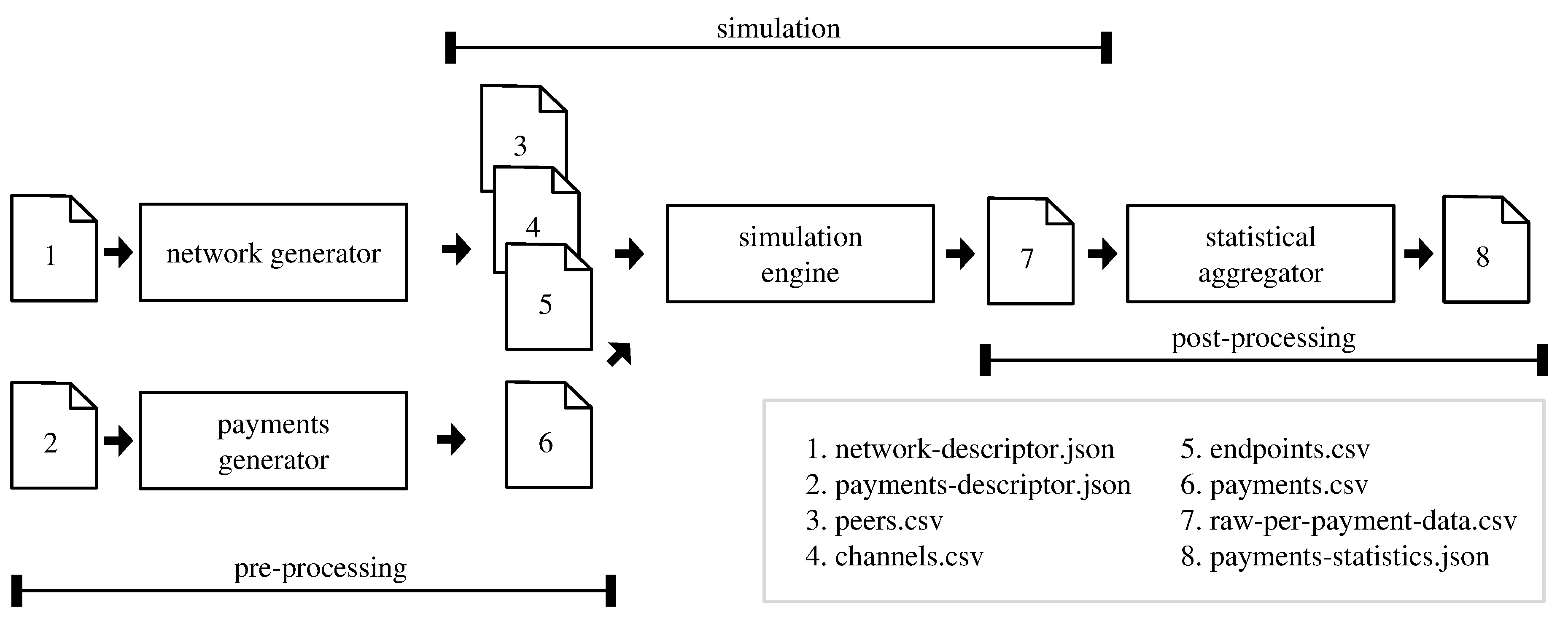
The workflow to interact with the CLoTH simulator is shown in Figure 4. It is composed by three phases: (1) pre-processing phase; (2) simulation phase; and (3) post-processing phase. For the sake of clarity, we first introduce the simulation phase. Then, the explanations of the pre-processing and post-processing phases follow.

4.3.1. Simulation Phase

Input attributes. The simulation engine requires two inputs:

• A complete specification of the HTLC network (Files 3, 4 and 5 in Figure 4). These files allow for a fine grained specification of the attributes of Figure 3 of peers (peers.csv), channels (channels.csv) and endpoints (endpoints.csv).
• The detailed list of payments to be executed with their attributes (File 6 in Figure 4, payments.csv), specifying sender, receiver, payment amount and triggering time.

Although verbose, this input specification allows for the most detailed definition of the simulation scenario. For a succinct and statistically meaningful input configuration mode, the reader can resort to the pre-processing phase of the workflow described below.

Simulation engine execution. Given the HTLC network and the payments specified as input, the simulation engine executes the payments on the HTLC network, running the actual discrete-event simulation.

Output attributes. The simulation phase outputs detailed information about each simulated payment (File 7 in Figure 4, raw-per-payment-data.csv):

• the end instant of the payment;
• the result of the payment: success or failure;
• the number of times the payment was attempted;
• whether the payment encountered an uncooperative peer; and
• the route traversed by the payment, if present.

4.3.2. Pre-Processing Phase

We wanted the CLoTH simulator to support fine-grained simulations as well as the possibility to concisely describe a simulation from a statistical point of view. While the input described in Section 4.3.1 directly supports the first case, the second requirement is fulfilled by the pre-processing phase. This phase takes as input a few parameters that statistically characterise both the network and the payments to be simulated. Then, it randomly generates an instance of HTLC network and an instance of payment script that match the input description.

Input parameters. Input parameters of the pre-processing phase with their symbols are shown in

Table 2. CLoTH simulator pre-processing phase input parameters.

Type	Symbol	Definition
Network	$N_p$	Number of peers
	$N_{ch}$	Average number of channels per peer
	${\sigma }_t$	Tuner of network topology
	$P_{{\overline{c}}_b}$	Uncooperative peers probability before HTLC establishment
	$P_{{\overline{c}}_a}$	Uncooperative peers probability after HTLC establishment
	$C_{ch}$	Average channel capacity
	G	Gini index of channel capacity
Payments	$r_{\pi }$	Average payment rate
	$N_{\pi }$	Number of payments
	${\sigma }_a$	Tuner of payment amounts
	$F_{sr}$	Fraction of same-recipient payments

. The following parameters deserve an explanation:

• ${\sigma }_t$ tunes the presence of hubs in the network topology. It is the width of the Gaussian distribution which defines the probability of connection among peers. In particular, for each peer, this Gaussian probability distribution is used for choosing the other endpoint of one of the peer channels. Therefore, if the width of this Gaussian is zero, all peers have one channel open with the same peer, which, consequently, will be an hub. On the contrary, if the Gaussian width is infinite, any peer has the same probability to be connected to any other, thus producing a totally decentralised network.
• ${\sigma }_a$ tunes payment amounts. It is the width of the Gaussian distribution whose tail is used to choose the orders of magnitude of payment amounts. The greater this width is, the longer the Gaussian tail is, and the higher the payment amounts.
• $F_{sr}$ is the fraction of the total payments directed toward the same recipient. Such parameter allows modelling the use case of many small payments sent to the same destination peer, e.g., to a provider of video-streaming services which is paid for each short segment of video streaming.

4.3.3. Post-Processing Phase

The post-processing phase transforms raw per-payment simulation output attributes into statistically meaningful performance measures (File 8 in Figure 4, payments-statistics.json). To do so, it applies the batch means method [19], which allows: (i) producing performance results that are not influenced by the initial transient state, where the system is not stable; and (ii) computing statistical mean, variance and 95% confidence interval for each measure. The batch means method consists in dividing a simulation run into multiple batches, which are statistically independent among each other. Output measures are zeroed and re-computed at each batch. Each final output measure is the statistical mean of that measure over the batches and comes also with variance and 95% confidence interval.

Simulation results format. The performance measures produced by the simulator are shown in

Table 3. CLoTH simulator performance measures.

Symbol	Definition
$P_s$	Probability of payment success
$P_{f_r}$	Probability of payment failure for no route
$P_{f_b}$	Probability of payment failure for unbalancing
$P_{f_{\overline{c}}}$	Probability of payment failure for uncooperative peers
$P_{\overline{k}}$	Probability of unknown payments
T	Payment complete time
$N_a$	Number of payment attempts
$L_r$	Payment route length

with their symbols. Some clarifications are presented in the following:

• $P_{f_r}$ is the probability that a payment fails due to the absence of a route connecting sender and receiver.
• $P_{f_b}$ is the probability that a payment fails because a channel in the route was unbalanced and an alternative route is not found.
• $P_{f_{\overline{c}}}$ is the probability that a payment fails because a peer in the route was uncooperative and an alternative route is not found.
• $P_{\overline{k}}$ represents the remaining fraction of payments for which we do not know whether they failed or succeeded, as they ended after the time validity window of our simulation. For example, this category can encompass payments delayed after a long timelock, as a peer was uncooperative after establishing the HTLC for the payment.
• T is the mean time for a successful payment to complete.
• $N_a$ is the mean number of times a payment is re-attempted.
• $L_r$ is the mean route length traversed by a successful payment.

4.4. Formal Model

Having a network with N nodes connected by payment channels and having M payments to be executed on this network, the simulator formal model can be expressed using the following formulas:

$$r_k=\varphi (p_k,{\mathcal{G}}_k,b_k)$$

(1)

$${\mathcal{G}}_{k+1}=\mu (p_k,r_k)$$

(2)

Function $\varphi$ is the function which finds a route for a payment. It takes as input the following parameters:

• $p_k=(n_{i_k},n_{j_k},a_k)$ for $k=1,2,\dots ,M$ is the payment for which a route has to be found: $n_{i_k}$ and $n_{j_k}$ are the sender node and the receiver node of the payment, for $i,j=1,2,\dots ,N$ and $i\ne j$; and $a_k$ is the payment amount.
• ${\mathcal{G}}_k$ is the graph of nodes $n_i$ for $i=1,2,\dots ,N$ connected by payment channels. The subscript k indicates the state of the graph at the moment in which $p_k$ is processed, with the available nodes and channels and their attributes at that moment.
• $b_k$ is the blacklist of possible nodes and channels excluded when searching for a route for $p_k$ (cf. Section 3).

The output $r_k$ is the route found for the payment $p_k$.

Given the payment $p_k$ and the route $r_k$, function $\mu$ executes the payment $p_k$ along the route $r_k$. Such function produces a new state of the graph, namely ${\mathcal{G}}_{k+1}$, because the payment execution causes some changes in the channels involved in the payment, such as the update of channel balances accordingly to the payment amount $a_k$.

4.5. Performance

Table 4. CLoTH simulator execution time: (a) as a function of the number of peers; and (b) as a function of the number of Dijkstra calls.

(a)
Peers	Execution Time (h)
100,000	6.64
200,000	15.92
500,000	49.25
700,000	64.68
1,000,000	104.15
(b)
Dijkstra Calls	Execution Time (h)
58,927	4.98
303,374	28.3

shows the performance of the CLoTH simulator in terms of execution time. Simulation times refer to experiments run on a machine of model DGX-1, manufactured by Nvidia, located in Rome, Italy. The machine is equipped with 80 CPUs of model Intel^® Xeon^® CPU E5-2698 v4 @ 2.20 GHz and 512 GB of RAM. Table 4a shows that execution time increases with the increase of the number of peers of the simulated network. This is due to the fact that time consumed by the Dijkstra’s algorithm, used to find payment routes, grows with the number of peers. With 1 million peers, a simulation run requires more than four days.

Table 4b shows that the execution time also increases with the increase of the number of calls to the Dijkstra’s algorithm. An execution of the Dijkstra’s algorithm is required each time a payment is attempted, so the more times the payments is re-attempted, the higher the number of calls to the Dijkstra’s Algorithm is, and the higher the simulation execution time is. The execution of the Dijkstra’s algorithm constitutes a bottleneck for the performances of the simulator. However, there are no limits on the values of the input parameters. The only effect of setting high values (e.g., an high number of peers or payments) is a correspondingly long execution time.

5. Simulation Experiments Design

In this Section, we present two groups of simulation experiments on HTLC payment networks:

• Simulations on the LN mainnet. In this set of simulations, we gave as input to the simulator peers and channels taken from a recent snapshot (downloaded on 14 June 2018 at 14:32 from LN explorer recksplorer) of the Lightning Network running on top of the Bitcoin main network (called mainnet, in the Bitcoin jargon). The goal of this set of simulations was to discover the cases (if any) in which a payment is more likely to fail than to succeed on the LN mainnet.
• Simulations on synthetic networks, i.e., HTLC networks generated by the network generator included in CLoTH (cf. Figure 4). The goal of these additional simulations was to study the impact of each individual input parameter on HTLC network performance. Therefore, this set of simulations took into account also the parameters defining the HTLC network, which were by definition fixed in the simulations of the LN mainnet.

The results of the study, i.e., performance measures under different network and payment configurations, are reported in Section 6.

5.1. Parameter Tuning

Each simulation experiment is defined by a set of independent variables. They are a subset of the simulator input parameters and attributes (input of pre-processing and simulation phases, respectively; cf. Section 4.3). The dependent variables are performance measures in the form of payment-related statistics, i.e., the output of the post-processing phase of the CLoTH simulator.

Variation Intervals

Each independent variable is studied in a proper variation interval. A variation interval is defined by its extreme values and by its sampling rate (i.e., the grain of its subdivisions, how many intermediate steps are considered).

Table 5. Variation intervals of the independent variables.

Variable	Interval	Unity of Measure
$N_p$	[100,000 200,000 500,000 700,000 1,000,000]	-
$N_{ch}$	[3 5 8 11]	-
${\sigma }_t$	[0 1 10 inf]	-
$P_{{\overline{c}}_b}$	[0 0.01 0.1 1.0 10.0]	%
$P_{{\overline{c}}_a}$	[0.01]	%
$C_{ch}$	[100 1,000 10,000 100,000 1,000,000]	satoshi
G	[0.0 0.1 0.2 0.4 0.6 0.8]	-
$r_{\pi }$	[10 100 1000]	payments per second
$N_{\pi }$	[10,000 100,000 1,000,000]	-
${\sigma }_a$	[1 2 3 4 5]	-
$F_{sr}$	[0 10 20 40 50]	%

shows the variation intervals for each independent variable.

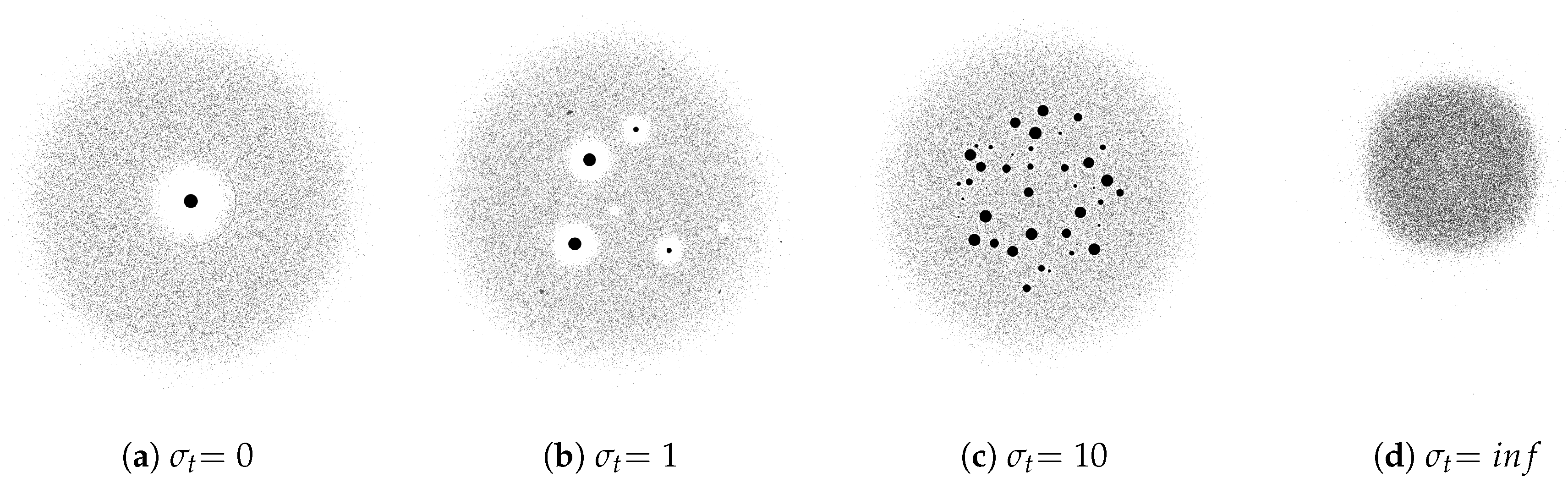
Regarding the topology tuner ${\sigma }_t$, Figure 5 shows the images of the resulting topologies for each of the values of the variation interval. In this Figure, node size is directly proportional to the number of open channels of the node. It can be noticed that: with ${\sigma }_t$$=0$, there is just one single big peer, which constitutes a centralised hub with many open channels; with ${\sigma }_t$$=inf$, instead, there are no hubs as all peers have the same size; and, with the middle values of ${\sigma }_t$, there are some scattered hubs.

Regarding the payment amounts tuner ${\sigma }_a$,

Table 6. Percentage of payments with a certain order of magnitude for each value of ${\sigma }_a$.

Order of Magnitude (Satoshi)	${\mathit{\sigma }}_{\mathit{a}}$
	1	2	3	4	5
${10}^{-3}$	67.83%	35.26%	26.33%	20.38%	18.00%
${10}^{-2}$	27.61%	29.57%	23.76%	19.85%	17.43%
${10}^{-1}$	4.3%	18.80%	18.40%	17.14%	15.53%
${10}^0$	2.6%	8.81%	13.79%	13.88%	14.14%
${10}^1$	0.0%	3.32%	8.80%	11.48%	11.49%
${10}^2$	0.0%	0.98%	5.08%	8.19%	9.69%
${10}^3$	0.0%	0.20%	2.58%	5.55%	8.19%
${10}^4$	0.0%	0.06%	1.26%	3.53%	5.51%

shows, for each value of ${\sigma }_a$, the payment amounts generated, in the form of: order of magnitude expressed in satoshi and fraction of payments whose amount has that order of magnitude. These are the orders of magnitude used for the simulations on the LN mainnet, while for the simulations on synthetic networks we increased by two each order of magnitude: the LN mainnet, in fact, being in its early stage of adoption, can tolerate only small payment amounts.

We ran some initial tuning simulations to define the intervals of the independent variables. We provide the rationales of each variation interval in the following:

• Number of peers $N_p$. A network with fewer than 100 thousands peers is too small, since the LN is supposed to scale Bitcoin. Regarding the upper limit, as shown in Section 4.5, a simulation with 1 million peers lasts more than four days, which is incompatible with the time constraints of our research activities (to be addressed in future research).
• Average number of channels per peer $N_{ch}$. With the tuning simulations, we noticed that with fewer than three channels per peer all payments fail, since the network is not properly connected. With 11 channels per payments, instead, no payments fail for absence of route, so performance would not improve with more than 11 channels.
• Topology tuner ${\sigma }_t$. The two limits, infinite and zero, correspond to the two opposite cases: totally decentralised and one single hub, respectively. The values in between are used to generate networks with some scattered hubs.
• Uncooperative peers probability before HTLC establishment $P_{{\overline{c}}_b}$. Regarding the choice of the upper limit, we deemed that a probability that a peer is uncooperative more than once every 10 times is unrealistic.
• Uncooperative peer probability after HTLC establishment $P_{{\overline{c}}_a}$. Payments failing for such uncooperative peers are not captured by our simulation since they end after the simulated time interval (because of the timelock). However, it is realistic to have this value different from zero, as it may happen with a certain small probability that a peer experiences a fault and goes offline after establishing an HTLC.
• Channel capacity $C_{ch}$. A channel capacity lower than 100 satoshis (which corresponds to $0.001 at writing time) would mean that the channel is unable to transfer anything but so-called dust payments. The upper limit is chosen in order to support the maximum payment amount and corresponds to one order of magnitude greater than such maximum.
• Gini index G. The Gini index is by definition a value between 0 and 1.
• Average payment rate $r_{\pi }$. A payment rate lower than 10 payments per second is not realistic for a world-wide payment system as LN aspires to be. The highest value is the average rate supported by mainstream traditional payment systems.
• Number of payments $N_{\pi }$. The values of this interval depend on the average payment per second, and on the fact that we force a simulation to last around 15 min (cf. Section 4.1).
• Payment amount tuner ${\sigma }_a$. The lowest value produces only small payments, but not lower than 1 millisatoshi (corresponding to $${10}^{-8}$ at writing time), to avoid dust payments (cf. Table 6). The highest value is to produce a certain fraction of high payments, however not higher than 0.001 BTC (less than $10), as the Lightning Network at least at this stage is not supposed to support large payments.
• Fraction of same-recipient payments $F_{sr}$. We consider unrealistic to send to the same recipient more than half of the total payments during a single simulation.

5.2. Simulations on the LN Mainnet

In this category of simulations, we set the input of the simulator using a recent snapshot of the LN mainnet. The goal of such simulations is to discover non-operative cases, i.e., cases in which the network is non-operative. We define the network as non-operative when it is more likely for a payment to fail than to succeed.

The only independent variables in this set of simulations are the payment parameters and the probability of uncooperative peers, as the other parameters are determined by the LN mainnet. For each independent variable we define:

• Non-stressing value: A value of the variation interval which is not supposed to negatively impact performance. For example, the non-stressing value for the uncooperative peers probability is zero, as in this case all peers are cooperative and do not cause payment failures.
• Stressing value: A value of the variation interval which is supposed to negatively impact performance. For example, the stressing value for the probability of uncooperative peer is 10%, as it is the highest probability of uncooperative behaviour specified in the variation interval.

Table 7. Stressing and non-stressing values of independent variables.

Variable	Non-Stressing Value	Stressing Value
$r_{\pi }$	10	100
$N_{\pi }$	10,000	100,000
${\sigma }_a$	1	5
$F_{sr}$	0%	50%
$P_{{\overline{c}}_b}$	0%	10%

shows the full list of stressing and non-stressing values for the independent variables of these simulations.

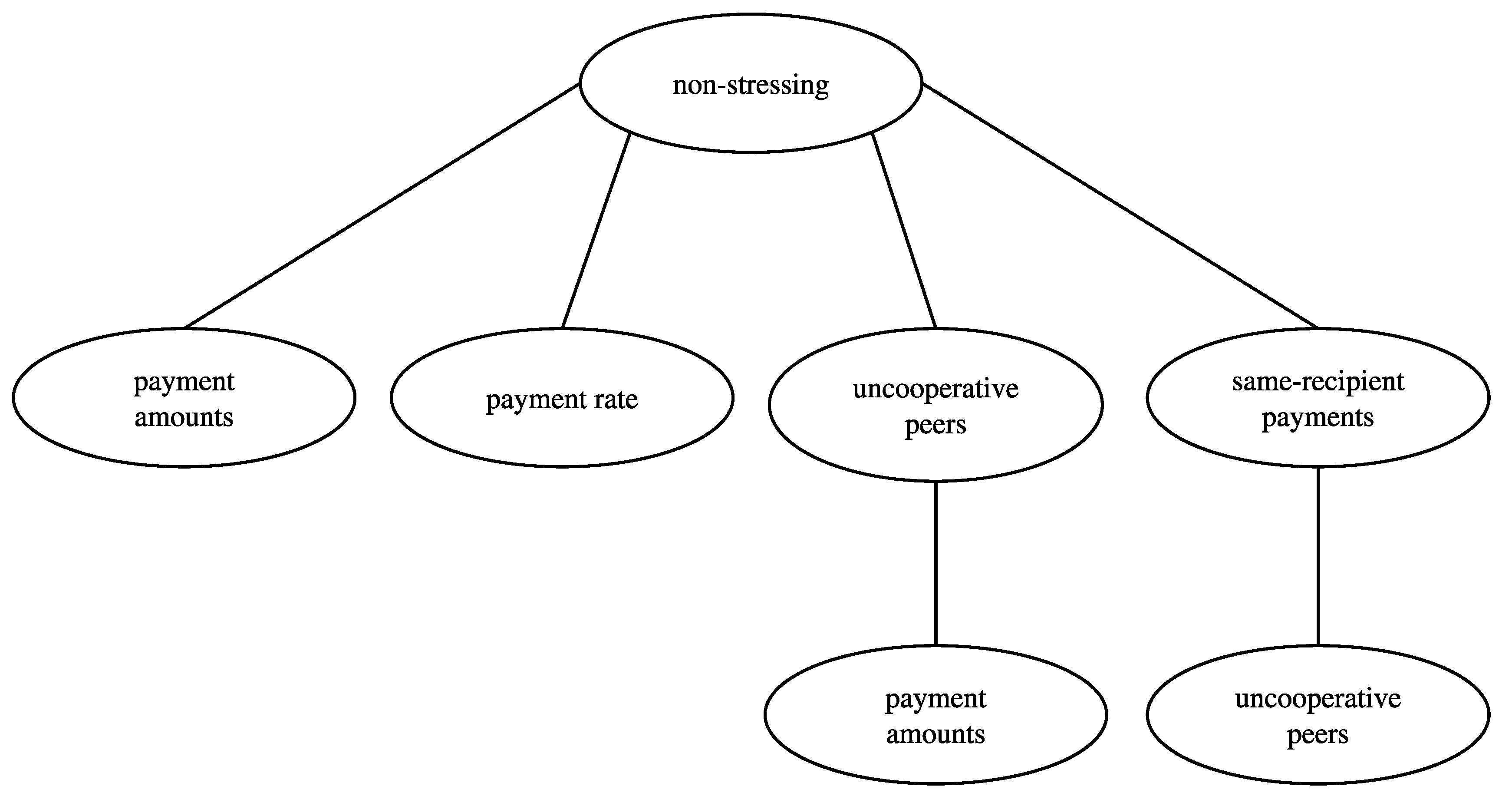
We adopted a branch-and-bound-like strategy to discover non-operative cases. The branch- and-bound tree of the simulations we ran is depicted in Figure 6. Each node represents a simulation, and the name of the node refers to the independent variable we stressed in that simulation. We proceeded in the following way:

• We started from the non-stressing simulation, where all variables are set to their respective non-stressing values.
• We stressed one individual independent variable at a time, thus forming a branch for each simulation with one stressed independent variable.
• If the simulation with the stressed variable produced a non-operative case, we stopped; otherwise, we continued examining that branch, stressing additional variables.

The formal algorithmic description of such strategy is shown in Algorithm 1, where $\mathcal{ST}$ represents the set of stressed independent variables and $P\left(\mathcal{ST}\right)$ the probability of payment success resulting from the simulation with the stressed variables in $\mathcal{ST}$.

Algorithm 1 Branch-and-bound-like strategy.

1: for each independent variable v do 2:       $\mathcal{ST}\leftarrow v$ 3:       for each independent variable $u\ne v$ do 4:             if $P\left(\mathcal{ST}\right)<50\%$ then 5:                  break 6:             else 7:                  $\mathcal{ST}\leftarrow \mathcal{ST}+u$ 8:             end if 9:       end for 10: end for

5.3. Simulations on Synthetic Networks

In this set of simulations, we study the effect on performance of one independent variable at a time. For each independent variable, we ran more simulations, one for each of its values in the variation interval. When studying a variable, the variables not under observation are set to a default value, i.e., a reasonable value in the interval for which that variable does not interfere with the results of the simulation. For example, for studying the effect of ${\sigma }_t$, we ran four simulations, one for each value of ${\sigma }_t$ defined in the variation interval (cf. Table 5); in each one of the four simulations, the other independent variables were set to their respective default values.

We did not adopt the branch-and-bound-like methodology for finding non-operative cases of synthetic networks because the resulting computational load would be too high. In fact, with eleven input parameters, the branch-and-bound-like strategy would require a very high number of simulations. We will pursue this direction in future work.

In the following, we explain the rationale of the chosen default values (shown in

Table 8. Default values of independent variables.

Variable	Default Value
$N_p$	100,000
$N_{ch}$	5
${\sigma }_t$	inf
$P_{{\overline{c}}_b}$	0%
$P_{{\overline{c}}_a}$	0.01%
$C_{ch}$	100,000
G	0.0
$r_{\pi }$	100
$N_{\pi }$	100,000
${\sigma }_a$	1
$F_{sr}$	0%

).

• Number of peers $N_p$. We did not choose a higher value because of the limited maximum execution time of the simulator; however, we performed a set of simulations varying the number of peers in the variation interval, to show the results for different values of such variable.
• Number of channels per peer $N_{ch}$. We used the value suggested by the LN developers [20].
• Network topology tuner ${\sigma }_t$. The chosen value produces no hubs in the topology, since the LN, as Bitcoin, is supposed to work in a decentralised topology.
• Uncooperative peers probability $P_{{\overline{c}}_b}$ and $P_{{\overline{c}}_a}$. The chosen values represent a realistic probability that a peer goes down for a fault.
• Channel capacity $C_{ch}$. The chosen value is higher than the maximum payment amount we used in the simulations.
• Gini index G. The chosen value produces a uniform distribution of bitcoins in the channels. In this way, performance is not influenced by an unbalanced distribution of bitcoins, where some channels have an high capacity and the others have a low one.
• Average payment rate $r_{\pi }$. It was set to the middle of the variation interval, neither too high nor too low.
• Number of payments $N_{\pi }$. It depends on the average payment rate, to ensure that the simulation does not last more the maximum duration allowed (15 min).
• Payment amount tuner ${\sigma }_a$. It was set to the lowest level possible in our interval, to avoid the performance being influenced by high amount payments, when the effect of payment amount is not under observation.
• Fraction of same-recipient payments $F_{sr}$. It was set to zero to avoid that such payments influence the performance in simulations in which their effect is not under observation.

6. Results and Discussion

In this Section, we present and discuss the results of both sets of simulations.

6.1. Simulations on the LN Mainnet

At the time of the snapshot, the LN mainnet presented the following features:

• Number of peers: 1221.
• Number of channels: 5167.
• Average degree (number of open channels per peer): 9.92.
• Average channel capacity: 381.35 satoshis.
• Gini index (concentration of bitcoins in channel capacities): 0.85.

As the reader can see, the LN mainnet is in its early development and adoption stage. It is small, as few peers and channels are present, and channel capacities are still low. Such premature state explains at least partially the non-operative cases found by our simulations.

We discuss the following simulations one branch at a time (cf. the branch-and-bound tree in Figure 6) to show the path we followed to discover non-operative cases. For each discussed branch, we show the results of the simulations corresponding to that branch, starting from the non-stressing simulation (the root of the tree), up to the last simulation in the branch (the leaf of the branch). The results of each simulation are presented in the following way: the values of the independent variables in that simulation, emphasizing the stressed ones; and the probability of payment success/failure that resulted from the simulation. The detailed results (which include all output measures) are available online.

6.1.1. Branch: Payment Amounts

In these simulations, we study the effects of stressing payment amounts. We started from the non-stressing simulation and then we ran a simulation in which we stressed ${\sigma }_a$. The results are shown in

Table 9. Simulation results of the branch of payment amounts.

Input Parameters				Output Measures
${\mathit{r}}_{\mathit{\pi }}$	${\mathit{\sigma }}_{\mathit{a}}$	${\mathit{F}}_{\mathit{s}\mathit{r}}$	${\mathit{P}}_{{\overline{\mathit{c}}}_{\mathit{b}}}$	${\mathit{P}}_{\mathit{s}}$	${\mathit{P}}_{{\mathit{f}}_{\mathit{r}}}$	${\mathit{P}}_{{\mathit{f}}_{\mathit{b}}}$	${\mathit{P}}_{{\mathit{f}}_{\overline{\mathit{c}}}}$
10	1	0.0%	0.0%	65.43%	24.40%	10.11%	0.0%
10	5	0.0%	0.0%	46.13%	46.11%	7.72%	0.0%

.

We found a non-operative case, as with a stressed ${\sigma }_a$ the probability of payment success turned out to be 46.13%, i.e., below 50%. Comparing the probabilities of payment failure between the non-stressing case and the amount-stressed case, we noticed an increase of the probability of payment failure for no route (46.11% against 24.40%), while the other probabilities of payment failure remain almost the same. This is due to the fact that capacities of channels are not enough to forward payments of higher amounts, thus a viable route for those payments is not found.

6.1.2. Branch: Payment Rate

In these simulations, we studied the effects of a stressed payment rate. Starting from the non-stressing simulation, we ran a simulation with a stressed payment rate (100 payments per second). The results are shown in

Table 10. Simulation results of the branch of payment rate.

Input Parameters				Output Measures
${\mathit{r}}_{\mathit{\pi }}$	${\mathit{\sigma }}_{\mathit{a}}$	${\mathit{F}}_{\mathit{s}\mathit{r}}$	${\mathit{P}}_{{\overline{\mathit{c}}}_{\mathit{b}}}$	${\mathit{P}}_{\mathit{s}}$	${\mathit{P}}_{{\mathit{f}}_{\mathit{r}}}$	${\mathit{P}}_{{\mathit{f}}_{\mathit{b}}}$	${\mathit{P}}_{{\mathit{f}}_{\overline{\mathit{c}}}}$
10	1	0.0%	0.0%	65.43%	24.40%	10.11%	0.0%
100	1	0.0%	0.0%	43.88%	25.17%	30.92%	0.0%

.

We discovered a non-operative case, as the stressed payment rate caused a probability of success of 43.88%. The cause is the increase of the probability of payment failure for unbalancing, which was around 20% higher with respect to the non-stressing simulation (30.92% against 10.11%). The reason of this result is that channel balances are depleted by the increased number of payments to be forwarded.

6.1.3. Branch: Same-Recipient Payments

In this branch, starting from the non-stressing condition, we firstly stressed the fraction of payments directed to the same recipient, set to half the total number of payments (5000 payments). The results in

Table 11. Simulations results of the branch of same-recipient payments.

Input Parameters				Output Measures
${\mathit{r}}_{\mathit{\pi }}$	${\mathit{\sigma }}_{\mathit{a}}$	${\mathit{F}}_{\mathit{s}\mathit{r}}$	${\mathit{P}}_{{\overline{\mathit{c}}}_{\mathit{b}}}$	${\mathit{P}}_{\mathit{s}}$	${\mathit{P}}_{{\mathit{f}}_{\mathit{r}}}$	${\mathit{P}}_{{\mathit{f}}_{\mathit{b}}}$	${\mathit{P}}_{{\mathit{f}}_{\overline{\mathit{c}}}}$
10	1	0.0%	0.0%	65.43%	24.40%	10.11%	0.0%
10	1	50%	0.0%	69.54%	18.81%	11.61%	0.0%
10	1	50%	10.0%	57.10%	18.80%	9.21%	14.84%

show that such stress did not worsen performance. The probability of payment success increased with respect to the non-stressing simulation (69.45% against 64.43%). Such increase is due to a decrease of the probability of payment failure for no route: from 24.4% to 18.81%. The reason for such behaviour is that the peer to which we directed half of payments has many open channels. Consequently, payments directed to this peer more probably found a viable route, with respect to the non-stressing case, in which payments were sent to different randomly-selected peers.

To make sure that we did not miss a non-operative case, we ran a further simulation stressing a second parameter. The only parameter we could stress was the probability of uncooperative peer. We could not, in fact, stress the payment amount, as the use case of payments directed to the same recipient is realistic only when such payments have low amount, and we could not stress the payment rate, since we already showed that with 100 payments every second the network was non-operative. The results of this simulation show that, with both $F_{sr}$ and $P_{{\overline{c}}_b}$ stressed (the latter set to 10%), the HTLC network remains operative. With respect to the case of only $F_{sr}$ stressed, the probability of failures for uncooperative peers increased to 14.84%, however, the probability of success is above 50% (57.1%), therefore the network resulted operative in this case too.

6.1.4. Branch: Uncooperative Peers Probability

In this last branch of simulations, we studied the effect of stressing the probability of uncooperative peers. The results in

Table 12. Simulation results of the branch of uncooperative peers probability.

Input Parameters				Output Measures
${\mathit{r}}_{\mathit{\pi }}$	${\mathit{\sigma }}_{\mathit{a}}$	${\mathit{F}}_{\mathit{s}\mathit{r}}$	${\mathit{P}}_{{\overline{\mathit{c}}}_{\mathit{b}}}$	${\mathit{P}}_{\mathit{s}}$	${\mathit{P}}_{{\mathit{f}}_{\mathit{r}}}$	${\mathit{P}}_{{\mathit{f}}_{\mathit{b}}}$	${\mathit{P}}_{{\mathit{f}}_{\overline{\mathit{c}}}}$
10	1	0.0%	0.0%	65.43%	24.40%	10.11%	0.0%
10	1	0.0%	10.0%	55.21%	24.31%	8.51%	11.92%
10	4	0.0%	10.0%	38.27%	46.10%	6.47%	9.13%

show that, when the only stressed value is the probability of uncooperative peers (set to 10%), the network is operative. In this case, the probability of payment failure for uncooperative peers is 11.92%, but the probability of payment success remains above 50% (55.21%); the other probabilities of failure are almost the same as the non-stressing case.

Again, to make sure that we did not miss non-operative cases, we stressed another parameter, the amount of payments (We did not stress the payment rate as we already showed that with 100 payments per second the network was non-operative and we did not stress the fraction of payments to the same recipient as we already studied this case (Section 6.1.3)). To stress the payment amount, we set ${\sigma }_a$ to 4 (not to 5, the highest possible level of payment amounts in the variation interval because we already show in Section 6.1.1 that with this value the network is not operative). The results of this additional simulation shows that stressing together the probability of uncooperative peers and the payment amounts, the network is non-operative: the probability of success, in fact, is 38.27%. The probability of failure for uncooperative peers is 9.14% (similar to the case in which the only stressed value was $P_{{\overline{c}}_b}$). Instead, the main reason of the failures is the absence of viable routes (with a probability of 46.1%), due to the increased amounts of payments.

6.1.5. Discussion of the Main Findings

Payment amounts. When we set ${\sigma }_a$ to 5, thus producing payments of the highest amounts (according to our interval and orders of magnitude, cf. Table 6), we discovered that the LN mainnet is non-operative, as the probability of success is only 46.13%. The main reason of the failure is the absence of viable payment routes, as the capacities of channels are not enough to forward payments of such amounts. While a naive solution would be to open channels with appropriate capacity, more elaborate approaches are beginning to appear, e.g., Atomic Multi-Path Payments [21], a technique that proposes to solve the payment amounts issue by splitting large payments into smaller ones which can be routed through channels with lower capacity, and then recomposed by the receiver.

Payment rate. Another non-operative case was found when we set the average payment rate to 100 payments per second. In this case, the probability of success was 43.88%. The main reason behind such a high failure rate is channel unbalancing: channel balances are depleted by an increased rate of payments to be forwarded. In addition, in this case, a naive solution would be to open channels with higher capacity, while a systemic alternative is represented by approaches akin to REVIVE [9], which allows channels to be re-balanced without the need of closing and re-opening them via on-chain transactions.

Uncooperative peers and payment amount. The last non-operative case resulted by the combination of a probability of uncooperative peers set to 10% and ${\sigma }_a$ set to 4. In this case, the probability of payment success was 46.1%; payments most likely failed for absence of viable routes, due to the payment amounts, then with probability 9.14% payments failed for uncooperative behaviour of peers. Such results allows us to conclude the following: First, the probability of uncooperative peers, as long as limited to the realistic value of 10%, does not constitute a serious problem for the network. Second, we proved once again that increasing payment amounts is the most critical issue for the LN configuration taken into account; a few recently proposed countermeasures are briefly mentioned above.

6.2. Simulations on Synthetic Networks

This set of simulations studied the effect on performance of each independent variable, one at a time. The simulations were run on synthetic networks whose parameters (together with the parameters of the simulated payments) were defined by the independent variables of our study. For each independent variable, we ran more simulations, one for each value of the variable in the variation interval, while keeping the other variables set to their default values (cf. Table 5 for the variation intervals and Table 8 for the default values).

The results show that the simulated synthetic networks are generally characterised by good performance: in almost all cases, in fact, the probability of payment success was around 99%. In this section, we present and discuss the most relevant results; the detailed results of all simulations are available online.

6.2.1. Channels Per Peer

In a decentralised network with 100 thousands peers, three channels per peer are not sufficient to have a robustly connected network. As shown in

Table 13. Simulation results varying the number of channels per peer.

${\mathit{N}}_{\mathbf{ch}}$	${\mathit{P}}_{\mathit{s}}$	${\mathit{P}}_{{\mathit{f}}_{\mathit{r}}}$	${\mathit{P}}_{{\mathit{f}}_{\mathit{b}}}$
3	59.61%	23.34%	16.77%
5	99.34%	0.31%	0.13%
8	99.82%	0.01%	0.0%
11	99.86%	0.0%	0.0%

, with three channels, the probability of payment success is 59.61%; payments failed for absence of route (with probability 23.34%) and because the few existing channels were unbalanced (with probability 16.77%).

With five channels per peer, instead, performance is good: probability of success, in fact, is 99.34%. With 11 channels per peer, the optimal condition is reached, as the probabilities of payment failure for no route and for unbalancing are zero.

6.2.2. Uncooperative Peers

As shown in

Table 14. Simulation results varying the uncooperative peers probability.

${\mathit{P}}_{{\overline{\mathit{c}}}_{\mathit{b}}}$	${\mathit{P}}_{\mathit{s}}$	${\mathit{P}}_{{\mathit{f}}_{\overline{\mathit{c}}}}$
0.0%	99.36%	0.0%
0.01%	99.34%	0.0%
0.1%	99.27%	0.1%
1%	98.32%	1.04%
10%	87.47%	11.84%

, if the probability of uncooperative behaviour of peers is 10%, the probability of payment failure for uncooperative peers is 11.84%. When $P_{{\overline{c}}_b}$ is lower, the network performance is not significantly affected by uncooperative behaviour, as the probability of payment success is around 99%.

6.2.3. Network Topology

The mean time to complete payments decreases as the network topology becomes more centralised. As shown by the results in

Table 15. Simulation results varying the network topology.

${\mathit{\sigma }}_{\mathit{t}}$	${\mathit{P}}_{\mathit{s}}$	T (ms)	${\mathit{L}}_{\mathit{r}}$ (hops)
0	99.88%	333.16	2.90
1	99.85%	536.83	4.13
10	99.83%	695.73	5.56
inf	99.34%	1391.92	10.34

, with one single hub (${\sigma }_t$ set to 0), mean payment time is 333.16 ms, while it grows to 1391.92 ms in a totally decentralised network with zero hubs (${\sigma }_t$ set to infinite). This is due to a corresponding decrease of the mean length of routes traversed by payments: with one single hub, almost each peer is connected to each other peer through the hub, so a route is on average long 2.90 hops, while it reaches 10.34 hops with zero hubs.

However, also in a totally decentralised topology the synthetic HTLC payment network is characterised by good performance: the mean time to successfully complete payments, in fact, is approximately equal to 1.4 s, i.e., nearly instantaneous, and the probability of payment success is 99.34%.

6.2.4. Same-Recipient Payments

As shown in

Table 16. Simulation results varying the fraction of same-recipient payments.

${\mathit{F}}_{\mathbf{sr}}$	${\mathit{P}}_{{\mathit{f}}_{\mathit{b}}}$
0%	0.13%
10%	0.13%
20%	0.12%
40%	0.10%
50%	16.06%

, when directing 50% of total payments (i.e., fifty thousands payments) to the same recipient, with a rate of 100 payments per second, the probability of failures for unbalancing reaches 16.06%. The reason is that channels direct to the destination peer unbalance, as they are traversed always in the same direction. Such unbalancing does not constitute a problem if fewer payments are directed to the same recipient: already with $F_{sr}$ set to 40%, the probability of payment failure for unbalancing decreases to 0.1%.

6.2.5. Discussion of the Main Findings

We found that synthetic networks performed well: the probability of payment success, in fact, is close to 99% in almost all cases. We proved that the values of the network parameters used in this set of simulations (e.g., the average channel capacity and the number of channels per peer) are good candidates as ideal reference values that network participants should actively try to maintain in a distributed effort to keep the network in good health.

In a decentralised network with 100 thousands peers, where each peer has only three active channels, a payment succeeds with probability 59.61%, i.e., much less than the 99% that can be reached with five active channels per peer. Therefore, at least five channels per peer are needed to have a robustly connected network.

If a peer is uncooperative once every 10 times, the probability for a payment to fail due to such uncooperative behaviour is 11.83%. Hence, the probability of uncooperative peers (unless unrealistically high) does not constitute a serious issue in our synthetic networks.

Payment mean time for a totally decentralised topology is approximately 1.4 s, i.e., nearly instantaneous. As to be expected, the presence of well-connected hubs acting as payment gateways further reduces the payment mean time.

Thousands of payments directed toward the same recipient in a short time window determine the unbalancing of channels involved, especially those closer to the payee. Merchants who expect to receive a significant payment throughput should open many payment channels (more than the default five), to prevent payment losses.

7. Conclusions

The present research work focused on the Lightning Network, the mainstream proposal that aims to address the well-known scalability problem of the Bitcoin blockchain. Such solution implements an HTLC payment network, i.e., a network to securely route off-chain payments through HTLC contracts.

We developed CLoTH, a simulator of HTLC payment networks. The simulator takes as input: (i) parameters representing the HTLC network to be studied (e.g., peers, channels, and channel capacities); and (ii) parameters defining characteristics of the payments to be simulated on the HTLC network (e.g., payment rate and payment amounts). CLoTH simulates the defined payments script on the input network and produces performance measures in the form of payment-related statistics (e.g., the probability of payment failures and the mean time to complete a payment).

Since the LN protocol focuses on anti-censorship objectives and each node of the network is free to join and leave, it is difficult to anticipate unexplored configurations of an HTLC payment network and therefore to actuate those interventions that may guarantee network health (quick and successful payments). In this sense, CLoTH is a valid predicting tool to simulate possible troublesome configurations and to check in advance the effects of a routing optimisation action (e.g., a node that joins the network, and then establishes and funds several payment channels).

We ran simulations on a recent snapshot of the HTLC payment network of LN. We identified those configurations in which it is more likely for a payment to fail than to succeed, thus defining an operative limit for the network. We also proposed countermeasures to avoid the occurrence of such configurations and mentioned recently proposed counteracting approaches. The non-operative configurations are a function of: payment amounts, payments rate, fraction of payments directed to the same recipient and the probability of uncooperative peers.

We also ran additional simulations on synthetic scenarios generated by statistical descriptions of HTLC networks and payment scripts. This second set of simulations aimed to separately study the impact on network performance of each individual CLoTH simulator input parameter. The results of these simulations show that the studied synthetic networks have good performance in most cases.

An analysis of the simulator execution led us to identify in the repeated local and inherently sequential application of the Dijkstra’s algorithm the performance bottleneck of the simulator. In our future work, we will address this limitation by distributing the computation on a cluster of machines. Simulator performance improvement will allow us to perform additional experiments to complete the coverage of the parameter space and to experimentally prove HTLC protocol limitations, if any.

References

- Nakamoto, S. Bitcoin: A Peer-to-Peer Electronic Cash System. 2008. Available online: https://bitcoin.org/bitcoin.pdf (accessed on 31 August 2018).
- Sompolinsky, Y.; Zohar, A. Accelerating Bitcoin’s Transaction Processing. 2013. Available online: http://citeseerx.ist.psu.edu/viewdoc/download?doi=10.1.1.433.6590&rep=rep1&type=pdf (accessed on 31 August 2018).
- Gervais, A.; Karame, G.O.; Wüst, K.; Glykantzis, V.; Ritzdorf, H.; Capkun, S. On the security and performance of proof of work blockchains. In Proceedings of the 2016 ACM SIGSAC Conference on Computer and Communications Security, Vienna, Austria, 24–28 October 2016; pp. 3–16. [Google Scholar]
- Poon, J.; Dryja, T. The Bitcoin Lightning Network: Scalable Off-Chain Instant Payments. 2016. Available online: http://www.cva-blockchain.org/wp-content/uploads/2017/08/lightning-network-paper.pdf (accessed on 31 August 2018).
- Decker, C.; Wattenhofer, R. A fast and scalable payment network with bitcoin duplex micropayment channels. In Symposium on Self-Stabilizing Systems; Springer: Cham, Switzerland, 2015; pp. 3–18. [Google Scholar]
- Miller, A.; Bentov, I.; Kumaresan, R.; McCorry, P. Sprites: Payment Channels that Go Faster than Lightning. arXiv, 2017; arXiv:1702.05812. [Google Scholar]
- Raiden Network. Available online: https://raiden.network/ (accessed on 31 July 2018).
- Burchert, C.; Decker, C.; Wattnhofer, R. Scalable Funding of Bitcoin Micropayment Channel Networks. In International Symposium on Stabilization, Safety, and Security of Distributed Systems; Springer: Cham, Switzerland, 2017. [Google Scholar]
- Khalil, R.; Gervais, A. Revive: Rebalancing Off-Blockchain Payment Networks. In Proceedings of the 2017 ACM SIGSAC Conference on Computer and Communications Security, Dallas, Texas, USA, 30 October–3 November 2017. [Google Scholar]
- Prihodko, P.; Zhigulin, S.; Sahno, M.; Ostrovskiy, A.; Osuntokun, O. Flare: An Approach to Routing in Lightning Network. 2016. Available online: https://bitfury.com/content/downloads/whitepaper_flare_an_approach_to_routing_in_lightning_network_7_7_2016.pdf (accessed on 31 August 2018).
- Vu, B. Exploring Lightning Network Routing. Available online: https://blog.lightning.engineering/posts/2018/05/30/routing.html (accessed on 31 July 2018).
- Bonneau, J.; Miller, A.; Clark, J.; Narayanan, A.; Kroll, J.A.; Felten, E.W. Sok: Research perspectives and challenges for bitcoin and cryptocurrencies. In Proceedings of the 2015 IEEE Symposium on Security and Privacy, San Jose, CA, USA, 17–21 May 2015; pp. 104–121. [Google Scholar]
- Croman, K.; Decker, C.; Eyal, I.; Gencer, A.E.; Juels, A.; Kosba, A.; Miller, A.; Saxena, P.; Shi, E.; Sirer, E.G.; et al. On scaling decentralized blockchains. In Proceedings of the International Conference on Financial Cryptography and Data Security, Christ Church, Barbados, 22–26 February 2016; pp. 106–125. [Google Scholar]
- Maximum Transaction Rate. 2016. Available online: https://en.bitcoin.it/wiki/Maximum_transaction_rate (accessed on 31 July 2018).
- Payment Channels. Available online: https://en.bitcoin.it/wiki/Payment_channels (accessed on 4 August 2018).
- C-Lightning. Available online: https://github.com/ElementsProject/lightning (accessed on 31 July 2018).
- Eclair. Available online: https://github.com/ACINQ/eclair (accessed on 31 July 2018).
- Lightning Network Specifications. Available online: https://github.com/lightningnetwork/lightning-rfc (accessed on 31 July 2018).
- Jain, R. The Art of Computer Systems Performance Analysis: Techniques for Experimental Design, Measurement, Simulation, and Modeling; John Wiley & Sons: Hoboken, NJ, USA, 1990. [Google Scholar]
- Vu, B. Lightning User Experience: A Day in the Life of Carol. Available online: https://blog.lightning.engineering/posts/2018/05/02/lightning-ux.html (accessed on 31 July 2018).
- Osuntokun, O. AMP: Atomic Multi-Path Payments over Lightning. Available online: https://lists.linuxfoundation.org/pipermail/lightning-dev/2018-February/000993.html (accessed on 31 July 2018).
Figure 1.
Multi-hop payment call graph of lnd.
Figure 2.
CLoTH simulator events state diagram.
Figure 3.
CLoTH simulator data structures.
Figure 4.
CLoTH simulator workflow.
Figure 5.
Resulting network topologies for different values of .
Figure 6.
Branch-and-bound-like strategy for simulations on the LN mainnet.