Development of an ANFIS Model for the Optimization of a Queuing System in Warehouses


1
Faculty of Transport and Traffic Engineering, University of East Sarajevo, Vojvode Mišića 52, 74000 Doboj, Bosnia and Herzegovina
2
Department of Logistics, Military academy, University of Defence in Belgrade, Pavla Jurisica Sturma 33, 11000 Belgrade, Serbia
3
NERI d.o.o. Ljesnica bb 74250 Maglaj, Bosnia and Herzegovina
*
Author to whom correspondence should be addressed.
Information 2018, 9(10), 240; https://0-doi-org.brum.beds.ac.uk/10.3390/info9100240
Submission received: 3 September 2018
/
Revised: 19 September 2018
/
Accepted: 21 September 2018
/
Published: 22 September 2018
(This article belongs to the Special Issue Multiple-Criteria Decision-Making (MCDM) Techniques for Business Processes Information Management)
Abstract
:Queuing systems (QS) represent everyday life in all business and economic systems. On the one hand, and there is a tendency for their time and cost optimization, but on the other hand, they have not been sufficiently explored. This especially applies to logistics systems, where a large number of transportation and storage units appear. Therefore, the aim of this paper is to develop an ANFIS (Adaptive neuro-fuzzy inference system) model in a warehouse system with two servers for defining QS optimization parameters. The research was conducted in a company for the manufacturing of brown paper located in the territory of Bosnia and Herzegovina, which represents a significant share of the total export production of the country. In this paper, the optimization criterion is the time spent in the system, which is important both from the aspect of all customers of the system, and from that of the owner of the company. The time criterion directly affects the efficiency of the system, but also the overall costs that this system causes. The developed ANFIS model was compared with a mathematical model through a sensitivity analysis. The mathematical model showed outstanding results, which justifies its development and application.
1. Introduction
In the daily performance of various activities and processes, logistics, as an integral and indispensable part of every business system, plays a very important role. It is necessary to rationalize the activities and processes that can significantly affect a competitive position of a company. A warehouse, as an individual logistics subsystem, together with transportation, represent the biggest causes of logistics costs, and there is a constant search for potential places of savings in these subsystems. Long ago, a warehouse was just a place used to separate surplus products, while its function today is completely different. Compared to the former static function, today’s warehouses represent a dynamic system in which the movement of goods is dominant. Therefore, in this paper, the emphasis is on the storage system of Natron-Hayat company, which is one of the largest companies in Bosnia and Herzegovina; this is sufficiently proved by the fact that it is one of the top five exporters of Bosnia and Herzegovina [1]. The current storage system of the company is decentralized, whereby each manufacturing facility has its own warehouse. Under such circumstances, there is the accumulation of demands for loading goods into vehicles and queuing, which again causes certain costs. In order to be successful in conditions of great competition, one of the most important segments is to satisfy the needs of customers, which is an integral part of a supply chain. Thus, it is necessary, according to Stević et al. [2], to optimize from the perspective of all participants in the complete supply chain. Today, customers pay more attention to the time they spend queuing; this time affects their decision about whether they will use the service again. This paper considers and analyzes the storage system of Natron-Hayat, a working group-warehouse paper machine (PM4), where arrivals of transportation means, queues, and service time depend on a number of factors. Throughout the research carried out in this paper, data on the arrivals of transportation means, which are registered at the weighing scale for loading in the PM4 warehouse, and the loading time for each vehicle, have been collected. Taking into account the capacities of all manufacturing machines in the company, the calculation of the basic parameters of the queuing system was conducted only for the PM4 warehouse, while the warehouses of the other manufacturing facilities were not taken into consideration at the moment. The PM4 storage system was into consideration, since it is a manufacturing machine with the largest capacity in the company; the company’s operations largely depends on its work, as can be seen in more detail in [3].
This paper has several goals. The first is to determine the state of the queuing systems of the company i.e., warehouse paper machine (PM4), which is the object of the research, by observing the system on a monthly basis. The second goal relates to the calculation of the system’s indicators by using a mathematical model. The third and most important goal of this research, which also represents a research contribution, is the development of an ANFIS model with three input variables: the inter-arrival time of trucks, the cumulative arrival time, and the service time (transloading-manipulative operations). The developed model provides meaningful information to all participants in the complete queuing system about the time in the system and the possibilities of its deviation, which can play an important role in planning and modeling the most important processes and business activities.
The proposed ANFIS model implies the union of all the advantages that the two artificial intelligence areas possess; the most important is the possibility of adaptation or learning from the example, and an approximate reasoning. Previous works provide an insight into the use of ANFIS in the field of traffic and transport, but in this paper, it is used in combination with the principles of queuing theory. Also, queuing theory is mainly based on analytical optimization models whose resolution can be complex. Numerous studies show the low sensitivity of ANFIS to inaccurate and incomplete input data, and its good ability to model non-linear dependencies, which is a characteristic of queuing systems.
In addition to introductory considerations where the basic reasons for the research are presented, the work is structured in five other sections. The second section provides a review of the literature referring to queuing systems and their optimization in different areas, as well as the application of ANFIS. Also, this section provides a literature review referring to multi-criteria decision-making methods (MCDM). The third section presents the methods in which a complete research algorithm is shown, by recognizing a need to perform it to the final goal. In addition, the basic settings of the QS and ANFIS models have been given. The fourth section provides a case study which consists of data collection and creation, and training of the model. Also, in this section the statistical inference of the distributions of input flow into the system and service time was determined. The fifth section contains the results and discussion. The sixth section provides a sensitivity analysis related to the QS mathematical model. The paper ends with conclusions in which the directions for future research are given.
2. Literature Review
This section is divided into three parts. The first is related to the application of the queuing systems theory and associated models in traffic and transportation. The second is oriented towards ANFIS models in this specific field, while the third refers to the overview of the application of multi-criteria analysis methods in traffic and transport.
2.1. Models of Queuing System Theory in Traffic And Transportation
Queues can occur wherever there is a need for the service of a large number of customers and the number of servers is limited. We encounter such situations in our lives every day, and taking into account that traffic and transportation affect the lives of every individual, queuing systems theory has a significant potential for application in this field. Every day, the number of transportation means is increasing on the streets, while the existing infrastructure, i.e., roads, does not undergo such a rapid expansion; consequently, traffic jams, waiting times on roads, travel time, costs increase, etc. In addition to these negative phenomena, from the ecological aspect, environmental pollution is also increasing. In order to optimize traffic flows, according to Guerrouahane et al. [4] and Raheja [5], exponential distribution of the inter-arrival time/general distribution of the service time/number of servers/system capacity systems are used for modeling. In [6], it is stated that highway flows are modeled as exponential distribution of the inter-arrival time/general distribution of the service time/one server, when there is no congestion, and as general distribution of the inter-arrival time/general distribution of the service time/number of servers in cases of congestion. The study [7] describes several different models for a traffic flow analysis, including exponential distribution of the inter-arrival time/exponential distribution of the service time/one server, in addition to those previously mentioned. Although queuing system theory is mainly used to model traffic flow on highways, intersections in large cities are bottlenecks, and can be modeled as exponential distributions of the inter-arrival time/exponential distribution of the service time/one server systems [8,9,10]. No matter which model is used, they all include a certain mathematical apparatus, i.e., mathematical models that are selected based on the system functioning (input flow, service flow). Therefore, not all are equally adequate for a particular system. Another example of applying the queuing system theory in traffic and transportation relates to the routing of transportation means in real-time. According to Chen [11], two strategies are given: FCFS (First Come First Served) and Median Repositioning, where the second one shows better results. The modeling of queues is also applicable to supply chains, where each sub-process is a queuing system. It is particularly important to optimize green supply chains by reducing fuel consumption, transportation time, and waiting time [12,13]. Warehouses can also be modeled using queuing theory. Some of the requirements that are imposed on optimization are shorter time of the implementation of operations, work with larger number of units of goods, the provision of the required quality of service, minimum costs. In addition, the application of queuing systems theory can be used to determine the size and capacity of a warehouse, and therefore, the necessary equipment within it [14,15]. Since the automation of warehouses is a trend nowadays, the AS/RS system (Automated Storage and Retrieval System) sets complex synchronization requirements that are resolved by queuing theory [16].
2.2. ANFIS Models in Traffic And Transportation
Intelligent transportation systems involve the application of various technologies, including artificial neural networks and fuzzy logic, i.e., neuro-fuzzy systems. Some of the basic objectives are to increase passenger safety, optimize routes, optimize the choice of means of transportation, reduce travel time, reduce costs, reduce traffic jams, waiting, etc. Using ANFIS models, a prediction of traffic flows in intelligent transportation systems can be performed. According to Bao-ping and Zeng-Qiang [17], the prediction model consists of 104 parameters that are adjusted during a training process. In order to increase safety, in research [18], ANFIS is used to assess the impact of intelligent transportation system technologies—such as video surveillance and drowsiness warnings—on the number of fatalities due to traffic accidents. Similarly, in [19], critical points on a road in rural areas are identified on the basis of collected data on traffic accidents. Traffic control at intersections with traffic lights can also be carried out using ANFIS models [20,21]. This involves reading out external data on the current state of the intersection, and forwarding them to the model that processes them and reacts in accordance with the learned rules [22]. From an ecological point of view, it is possible to estimate the noise level, as indicated in [23]. Traffic flow density, vehicle speed, and the noise level of horns can be taken as input independent variables. The selection of an optimum transportation route using the ANFIS model, based on the criteria specified by the dispatcher, is considered in [24], while [25] deals with a choice of an optimum mode of transportation. Warehousing is an important part of the entire supply chain. It can be said that the efficiency of a warehouse affects the overall efficiency of the chain, and therefore, requires intelligent optimization solutions. [26] deals with determining the number of forklifts in a warehouse which are required for loading goods using an ANFIS model, based on a given number of pallets and time available. Another example of the implementation of expert knowledge in an ANFIS model for using forklifts is presented in [27].
2.3. Methods of Multi-Criteria Decision-Making in Traffic And Transportation
Multi-criteria decision-making can be used as an adequate tool for making valid decisions. In [28], the EMDS (Ecosystem Management Decision Support System) and SADfLOR (Web-Based Forest and Natural Resources Decision Support System) imply the integration of multiple approaches to determine optimal bundles of ecosystem services. In traffic and transport, the role of MCDM (Multi-Criteria Decision Making) is of paramount importance. For the determination of optimal locations, spatial information obtained by the GIS (Geographic Information System) is often used with multi-criteria decision making [29]. Karczmarczyk et al. [30] represents the application of the novel method, COMET (Characteristic Objects Method) to determine the best model of the electric car for sustainable city transport with respect to increasing pollution in cities. The same method was used in [31] for the selection of the best scenarios for the transport of dangerous goods. With the aforementioned COMET method, the theory of the fuzzy sets for the modeling of imprecise data is used. The supply chain involves a large number of participants, and with the correct choice of suppliers, at the initial stage, good conditions for optimizing the entire process are created. Stevic et al. [2] developed a new approach: Rough EDAS (Evaluation based on Distance from Average Solution), Rough COPRAS (Complex Proportional Assessment) and Rough MULTIMOORA (Multi-Objective Optimization by Ratio Analysis Plus the Full Multiplicative Form) to solve the problem of correct choice of suppliers. In [32], a model of dynamic or temporal choice of a supplier is proposed using multi-criteria decision making. The observed neuro-fuzzy system, ANFIS, finds its application in the field of decision-making on the basis of several criteria. Khalili-Damghani et al. [33] divides the process of selecting suppliers in two phases, the first of which involves the application of ANFIS to determine the overall usefulness of the supplier based on expert knowledge. According to Torquaybade [34], in the supply chain optimization, ANFIS has the role of assessing the performance of each of the Pull Control Policies based on the input variables. A multi-criteria approach was also applied in [35] for the identification of priority black spots in order to increase the safety in traffic. The applicability in the field of traffic engineering of the MCDM methods is also confirmed in paper [36], where it is used for the evaluation and selection of roundabouts in an urban area.
3. Methods
The first step of the research is data collection, i.e., the values of selected variables that will be used first for statistical analyses, and then for the creation and training of the model based on fuzzy logic and artificial neural networks. The basic method used for the realization of the research is modeling. In addition, a statistical method is used, as well as theoretical analysis explaining basic concepts and principles of queuing systems and the ANFIS model. Used software packages, such as MATLAB, Minitab, and EasyFit, make the application of these methods much easier.
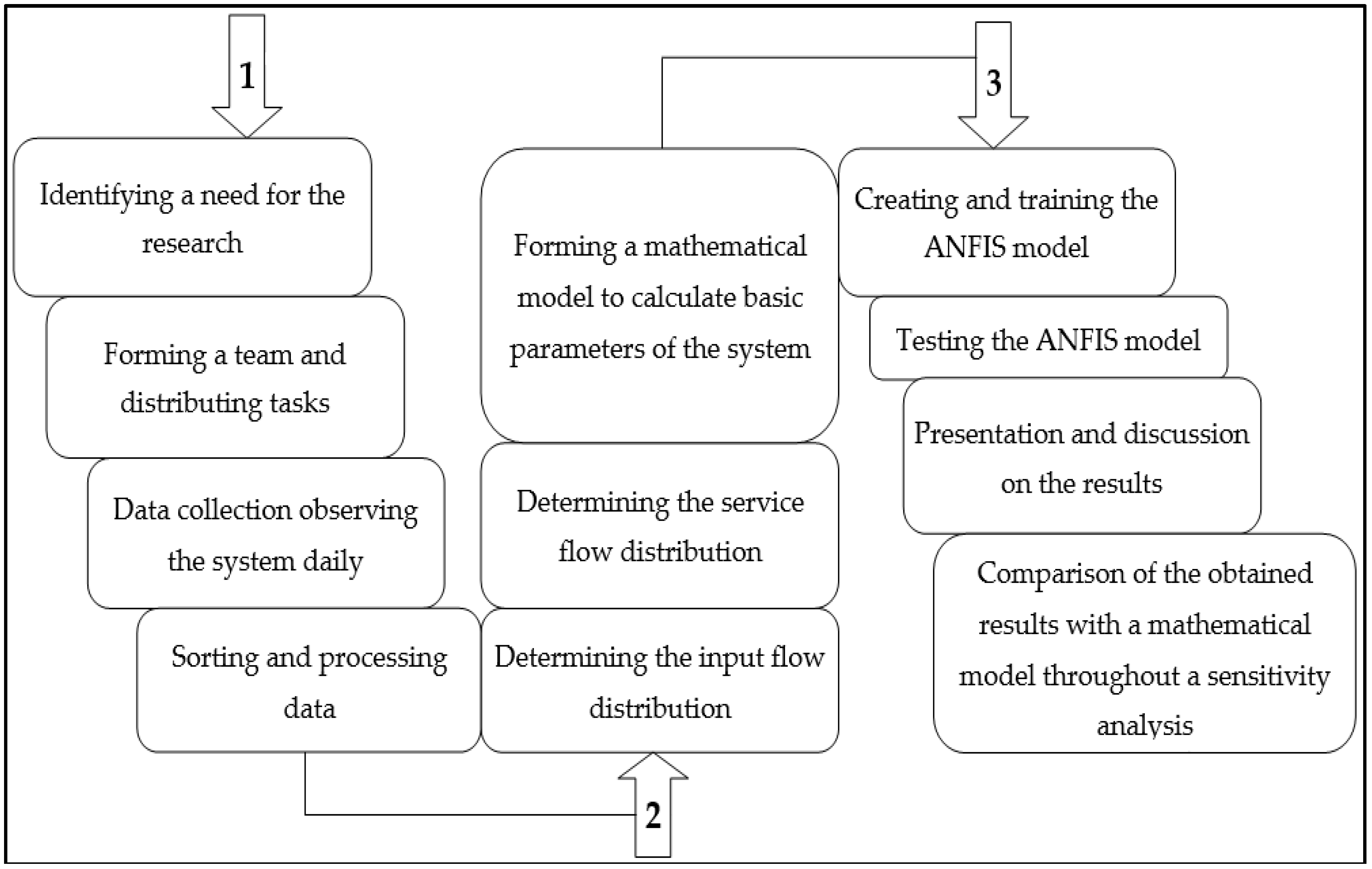
Figure 1 shows the proposed model in the study. It consists of a total of three phases and 11 steps. The first phase includes four steps: the first relates to the recognition of the need to conduct research that will help both customers (transportation companies) and the company’s management increase the efficiency of their business. The second step is the formation of a team and the distribution of tasks, as well as counseling with staff at a tactical level on how to interact with the system, i.e. collect data, which is the third step of this phase. In the final step of the first phase, the sorting of data collected, and their processing, are performed. The second phase consists of three steps. The first two relate to determining the distribution of the input flow and the flow of service, respectively, while the third involves the formation of a mathematical model in the Minitab software for the calculation of the basic parameters of the system. The third phase includes the development of the ANFIS model, discussion of the obtained results, and a comparison with a mathematical model.
3.1. Basic Principles of Queuing Systems Theory
Today, queuing theory has a very wide range of applications in many branches of human activity where customers come into a system, by some mathematical distribution, due to a particular service, and in the case of occupied servers, form one or more queues. Upon the completion of service, where its time also corresponds to some distribution, the customer leaves the system. Such examples can be seen daily in traffic, logistics systems, banks, post offices, in telecommunications traffic, at a gas station, etc. Naturally, situations that are more complex are possible when a customer passes throughout a network of interconnected queuing systems. The task of queuing systems theory is to explain and model the behavior of such systems using a mathematical apparatus. In addition to other methods, it is widely applicable to operational research [37]. Modeling a queuing system enables the analysis and optimization of its performance.
As the basic features of the queuing systems model, the following can be identified: the input process, service mechanism, and queue discipline [38]. According to Maragatha and Srinivasan [39], every model can be described using the following features:
- The distribution of inter-arrival time; this most often corresponds to a Poisson, exponential or general distribution. Arrivals can be individual or in groups [40].
- The distribution of service time: exponential, hyper-exponential, hypo-exponential, constant, general.
- The number of servers can be one or more.
- The length of queue can be precisely defined or infinite. In case of arrival when the queue capacity is maximally filled, the costumer is denied, which is known as ‘balking’.
- System capacity implies the maximum number of customers in the system, being served or in the queue.
System disciplines:
- FIFO (First in, First out)—in the order of arrival,
- LIFO (Last in, First out)—a customer that comes last will be served first,
- Random Service—customers are served in random order,
- Round Robin—a customer gets a time slot within which he/she will be served. If the service is not completed, the customer returns to the beginning of the queue,
- Priority Disciplines—the order of customer service is determined according to the priority that each one receives [37].
The Kendall notation uses these six features to describe the queuing system:
where
A/B/m/K/n/D
- A—the distribution of the inter-arrival time,
- B—the distribution of the service time. Positions A and B can be replaced by M (Markov processes, exponential distribution); D (deterministic distribution); E (Erlang distribution); H (hyper-exponential distribution); G (general distribution),
- m—the number of servers,
- K—system capacity,
- n—population size,
The most common and simplest queuing systems are of M/M/m type.
3.2. Adaptive Neuro-Fuzzy Inference Model
Unlike biological neural networks, artificial neural networks represent an attempt to model the human brain through modern computing. They consist of a number of process elements, or artificial neurons, which are analogous to the brain, in which the basic elements are nerve cells. Artificial neurons, as well as nerve cells, are characterized by parallel work in the processing of various types of information [42]. Their basic feature is the ability to learn, which means that it is necessary to first train the network to efficiently perform tasks such as recognizing shapes, images, speech, function approximation, prediction, optimization, data clustering, processing inaccurate and incomplete data, etc. Accordingly, the basic task of an artificial neural network is to combine different inputs, and to process and forward signals to one or more outputs. There are various types of artificial neural networks depending on the number of neurons, i.e., layers, network training methods, the way to transmit signals throughout the network, etc.
Fuzzy technologies allow the computer to work with uncertainties, thereby achieving a similarity with the human way of thinking. Fuzzy logic is an extension of classical logic in which variables can have only two values: correct (1) and incorrect (0). In this way, variables can occupy any real value between 0 and 1. Fuzzy sets are basic elements for presenting and processing unclear things and uncertainties in fuzzy logic, and they are mathematically presented by membership functions. The inference system in fuzzy logic implies defined membership functions of individual variables and inference rules, which connect input variables with an inference; they are called IF-THEN rules.
The systems that integrate the principles of artificial neural networks and fuzzy logic are called neuro-fuzzy systems. They use a learning ability of artificial neural networks based on training data in order to adapt the forms of membership fuzzy functions and inference fuzzy rules. In this way, in one system, the advantages of logical inference and learning are combined. One of the most commonly used neuro-fuzzy systems is ANFIS (Adaptive Neuro-Fuzzy Inference System). ANFIS is a multilayer neural network that, based on data (input-output vector) for training, provides a certain value of an output variable for certain inputs. An important feature is that ANFIS can effectively model nonlinear connections of inputs and outputs [43]. ANFIS training is based on the application of an algorithm of error propagation backward, either alone or in combination with the method of least squared error, i.e., hybrid algorithm [44]. ANFIS uses the Takagi-Sugeno method of inference, and a typical fuzzy rule, assuming two inputs (x and y) and a logical AND operation, can be written as follows:
IF x is A AND y is B, THEN z = f(x,y)
A and B denote fuzzy sets of input variables x and y, while z is an output function.
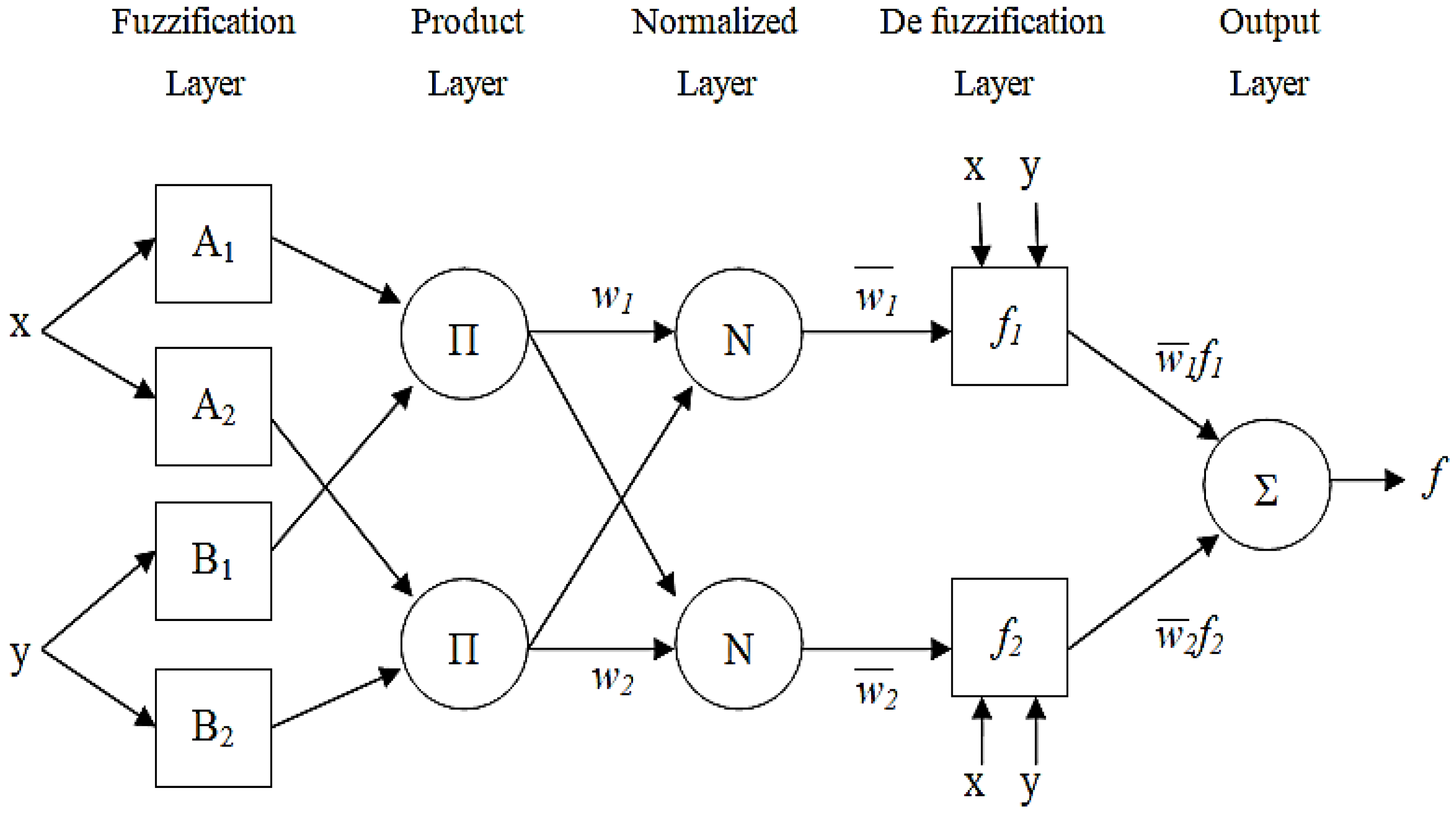
The ANFIS structure consists of five layers, as shown in Figure 2. The nodes of the first layer define fuzzy sets, i.e., membership fuzzy functions corresponding to input variables. This layer is often called a fuzzification layer, because it determines the membership degree of the value of a variable to a particular fuzzy set [45]. The nodes of this layer are adaptive, which means that their parameters are adjusted during a training period [44]. The first-layer nodes that represent the membership functions of the input variable X can be defined as , where j (j = 1 ,..., 2) denotes the number of membership functions [46].
The second-layer nodes are fixed and perform an operation of multiplying the input signals (operation AND). The ith neuron has the output of the form: . The output of the second layer is equal to the minimum value of the two inputs [47].
The third layer normalizes the values obtained at the output of the nodes of the second hidden layer. In the case shown in Figure 2, with two nodes in the second layer, the normalized value at the output of the ith node of the third hidden layer has the following mathematical form:
Each node of the fourth layer is an adaptive node with the function it completes, which can be written as follows [48]:
where pi, qi and ri are inference parameters. The fifth layer calculates the output as a sum of all input signals:
The set of fuzzy inference rules that apply to the structure given in Figure 2 consists of two rules:
IF x is A1 AND y is B1, THEN f1 = p1x + q1y + r1
IF x is A2 AND y is B2, THEN f2 = p2x + q2y + r2
ANFIS is most often trained with a hybrid algorithm. It requires two passes through the network in each epoch. In the forward pass, a method of least squares is used to modify the parameters of the linear functions of rule inferences (layer 4) [34]. When going backward, the parameters of fuzzy membership functions of input variables (layer 1) are modified by the algorithm of error back-propagation.
4. Case Study
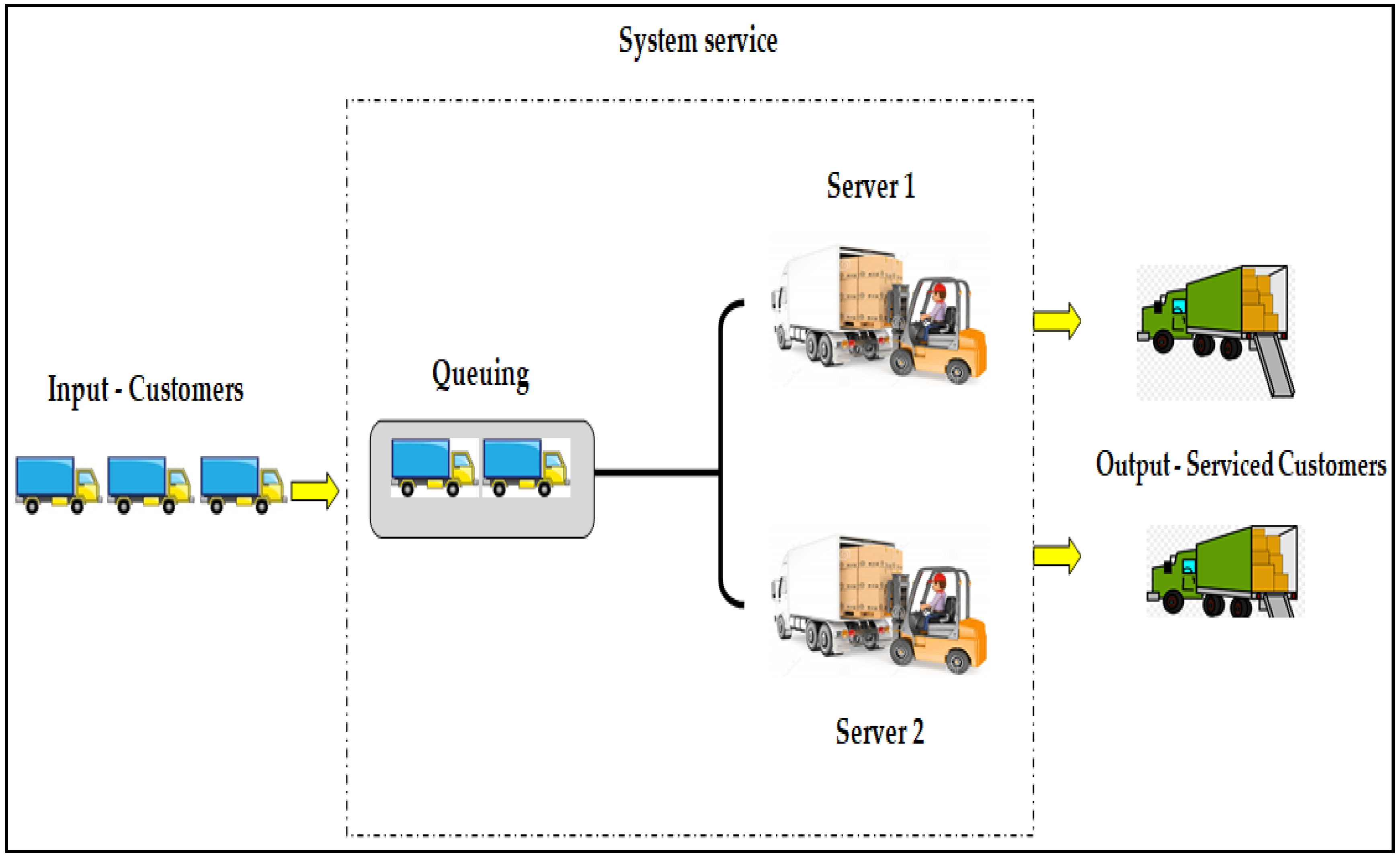
Figure 3 shows the basic processes of the QS at Natron-Hayat for the PM4 storage system. The road freight transportation means of different companies represent customers of the system. They enter the system with a certain intensity. Upon entering the company’s property, they form a queue depending on the current service intensity. There are a total of two transloading fronts (servers) where forklifts are engaged in the loading of goods. The queue formed and servers represent the service system, while loaded vehicles are serviced customers.
4.1. Data Collection
In order to model the queuing system of the PM4 working group of Natron-Hayat, it was necessary to collect data on the basic features of the system. The values of the following variables were monitored:
- the inter-arrival time of trucks,
- the cumulative arrival time since an initial time (for each day),
- the service time (transloading-manipulative operations) and
- the time in the system.
The first three listed variables represent the input variables of the ANFIS model that predicts the time spent in the system. Therefore, it is clear that time represents the output variable, taking into account the well-known fact that the time in queuing systems is one of the most important criteria for optimizing and modeling them.
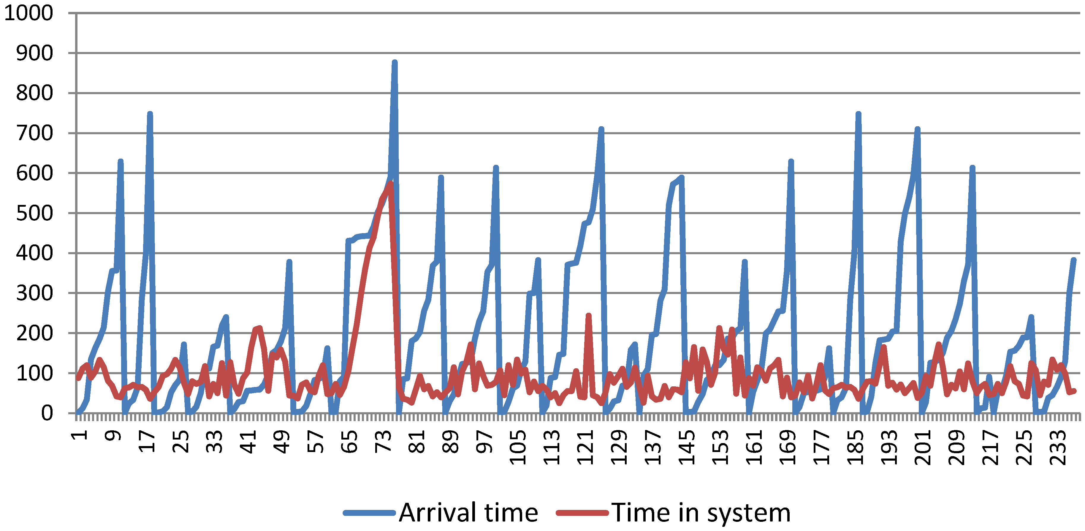
The data collection period lasted 11 working days in two shifts of 8 h, based on which a monthly report was received for 22 working days, which means a total of 352 h. A total of 237 trucks entered the system. Out of the total set of data, the values of the seventh day of monitoring are excluded, after 2 p.m. to the end of working hours. The reason is the emergence of unusual and extremely high values of time spent in the system during the arrival of trucks at the end of the first and the beginning of the second shift. Such values adversely affect the performance of the ANFIS model. Figure 4 graphically shows the time spent in the system and the cumulative arrival time for each truck, as well as the given deviations occurring from the arrivals of the 65th to the 76th truck.
In addition to the extreme deviations, the values of variables for the 122nd truck that entered the system due to the extreme value of the service time of 240 min were neglected. The time of its arrival in the system is in the 8th hour on the last day of data collection, so that period was also omitted. The final set of data, which is statistically analyzed and used to create the ANFIS model, is reduced to the time of 352 h, during which 224 trucks entered the system.
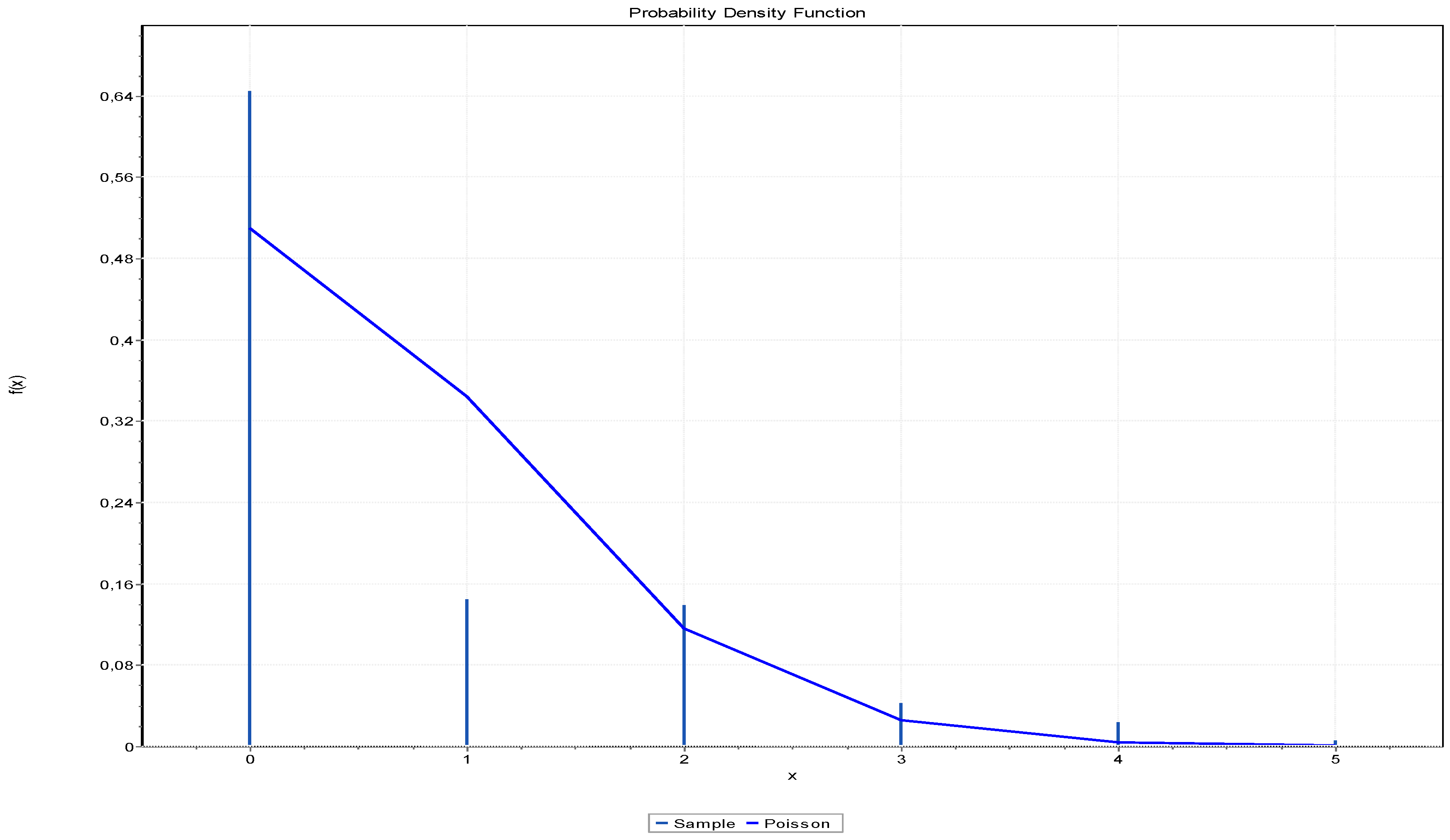
The examination of the input flow, i.e. the arrivals of trucks in the system, is essential for determining the distribution of the probabilities of inter-arrival time and the distribution of probabilities of the arrival of certain number of trucks at a given interval. Table 1 gives frequencies related to the number of trucks that arrived in a period of one hour. The biggest frequency is 214, when no truck entered the system during one hour. For a larger number of trucks that arrived in one hour, frequencies of hours were reduced, so in the end, the largest number of trucks that arrived during one hour was five, and with a frequency of two.
Based on Table 1, a statistical procedure is used to determine the distribution of the input flow. The EasyFit software provides graphical and tabular results for the procedure to determine the best fitting of data with a particular distribution. Figure 5 shows the Poisson distribution that best fits the input flow. The distribution parameter is λ = 0.6747, which represents the arrival intensity of the number of trucks within one hour.
Table 2 gives an overview of the completed statistics of the Anderson Darling (AD) test for determining data fitting to a particular distribution. The Poisson distribution is ranked as the best in the Anderson Darling test with the statistic of 88.26. A total of 8 distributions are given, but it is possible to determine the fitting only for Poisson, Geometric, and D. Uniform.
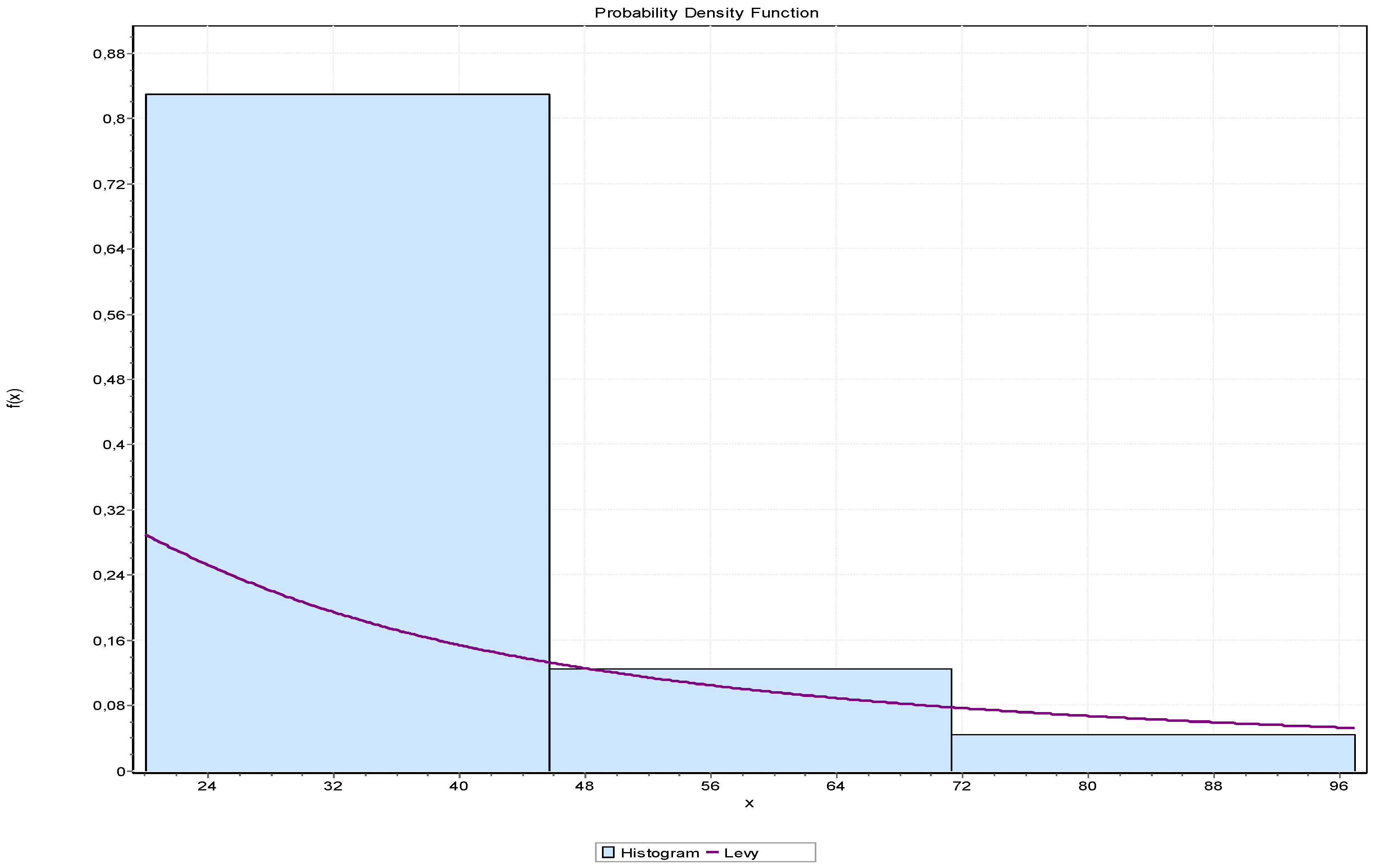
In order to determine the distribution of service time, it is necessary to divide the data into classes. Taking into account that the maximum value of service time is 95 min, and the minimum is 15 min, a division into 8 classes per 11 min of duration is performed. Table 3 shows the number of trucks that is served within a certain interval (class). The largest number of trucks is served within the class with the limits between 26 and 36 min, while no truck is served from 70 to 80 min.
Figure 6 shows the Levy distribution curve that best fits the service time frequencies presented in Table 3. The probability density function of the shown distribution can be expressed as follows:
where the parameters, in this specific case, are and . The average service time is 38.62 min, which means that the service intensity is trucks/hour.
Table 4 presents the values of ranges and the statistics of the Anderson Darling test for testing the fitting of service times to certain distributions. Results are given for 8 distributions, and Levy is ranked as first, with a statistic of 1.5611.
As mentioned, we used the software Easyfit to obtain the statistical distributions. This software supports Kolmogorov-Smirnov (KS) and AD tests. We used the AD test, because it is better, and according to Engmann and Cousineau [49], it has two extra advantages over the KS test. First, it is especially sensitive to differences at the tails of distributions. Second, there is evidence that the AD test is more capable of detecting very small differences, even between large sample sizes. This is one of its main advantages in the field of engineering. Also, the KS test is less able to detect changes in asymmetry, requiring almost twice as many data compared to the AD test. Finally, this test, according to Stephens [50], is a good all-purpose test. The AD test is also used in [51,52].
4.2. Creation and Training of the Model
Creation, training and testing of the ANFIS model is performed in the MATLAB software package, which, thanks to the graphical user interface of the ANFIS editor, allows easy manipulation of the model’s parameters and variables. As a result, a large number of graphic displays of parameters and performance are obtained.
The total set of data on the inter-arrival time, cumulative arrival time, service time, and the time spent in the system for each truck that enters the system, is divided into three parts:
- Training data, consisting of 73.21% or 164 input-output vectors, providing the so-called “Learning with a teacher”, where the outputs from the network are known in advance for appropriate inputs.
- Checking data, which is primarily aimed at preventing the occurrence of training data overfitting. The ANFIS model monitors the value of the checking error in each training epoch and retains learned parameters at its minimum value. Checking data consists of 13.39% or 30 input-output vectors.
- Testing data enables us to perform an evaluation of the abilities of the ANFIS model to perform a prediction of the time spent in the system as accurately as possible. The outputs of the ANFIS model are compared with known values, and the goal is to select a model that makes a minimum error. As well as checking data, testing data consists of 13.39% of the total set of data.
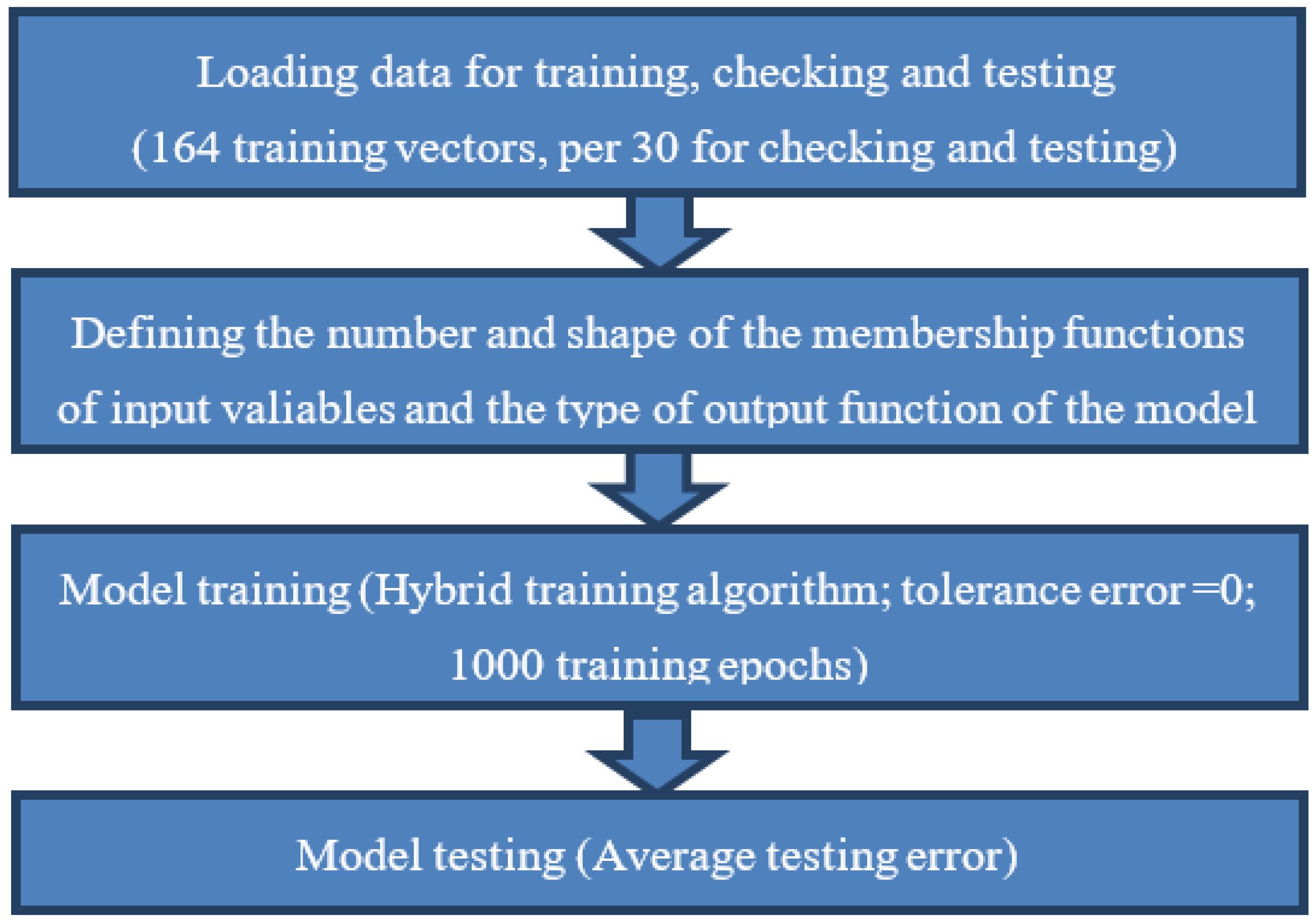
The process, from creation to model testing, can be summarized by the algorithmic steps given in Figure 7.
5. Results and discussion
The ANFIS model performance is estimated based on an average testing error, which in fact is an average square error-RMSE (Root Mean Square Error), and is calculated as:
where N is a number of testing vectors, n(k) is expected (measured) value, and is the value obtained by the model. Table 5 gives an overview of RMSE values depending on the shape and number of fuzzy membership functions for each of the three input variables for the constant shape of the output function. The values of the average testing error for different ANFIS models in the case of a linear shape of the output function are given in Table 6. The model training was carried out in 1000 epochs. With a larger number of membership functions, the average testing error increases, so that a maximum of three are considered here. Table 5 gives an overview of RMSE values depending on the shape and number of the membership fuzzy functions for each of the three input variables for the constant shape of the output function.
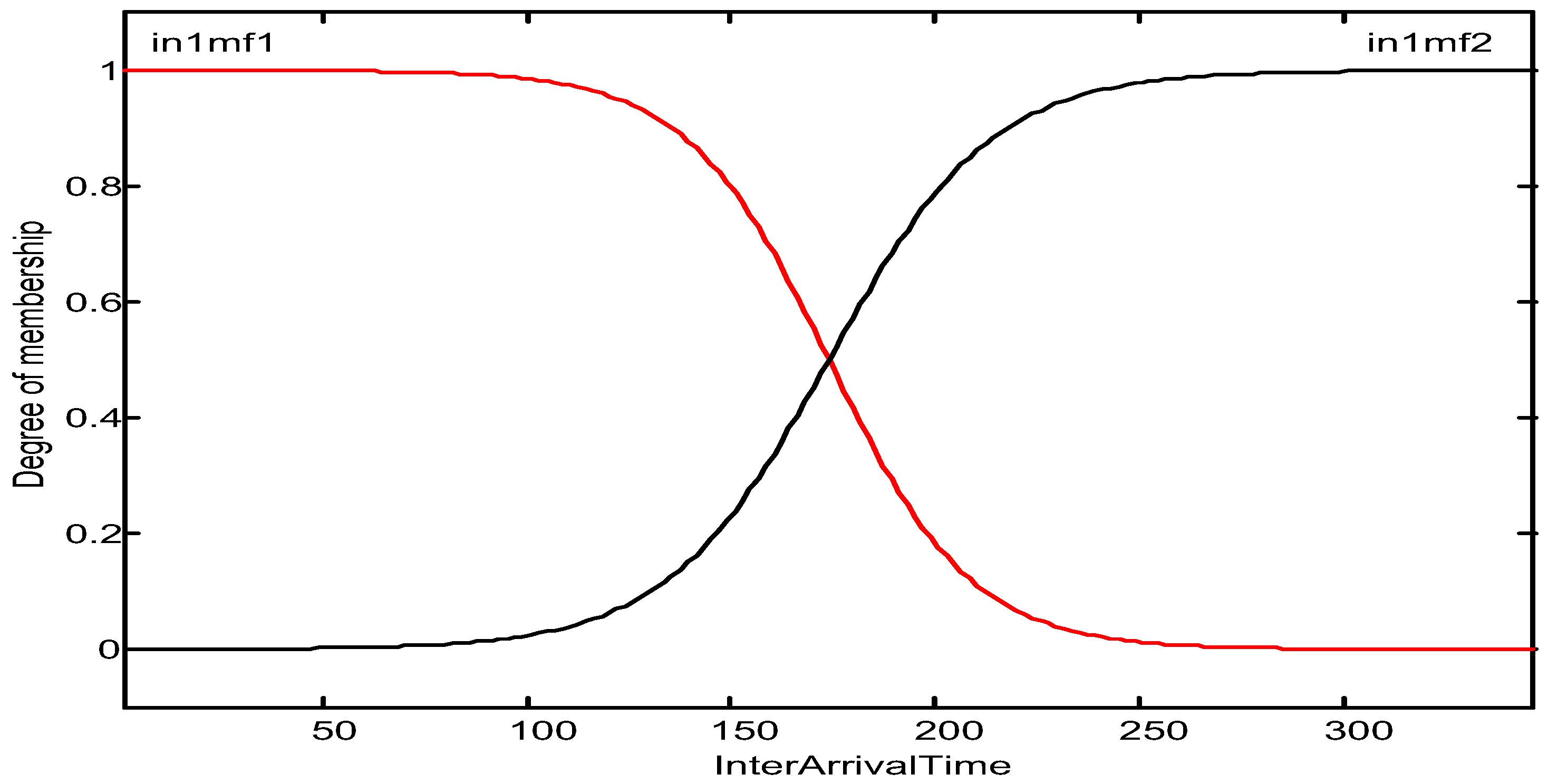
By comparing the values in Table 5 and Table 6, it is concluded that the linear output model gives drastically higher error values than the constant output shape. The least average testing error from Table 6 is 25.42 min, and from Table 5, 13.67 min. Therefore, a model with a lower error is selected from Table 5, which has two fuzzy membership functions for each input variable. The functions are in the shape of dsig, and represent the difference of two sigmoid functions, which can be written as follows:
Since it relates to the difference, the dsig function has four parameters: a1, a2, c1, and c2. Figure 8 shows the certain membership functions for the first input variable-inter-arrival time. The learned parameters of the first function marked by red color in Figure 8 are 0.0578, −172, 0.0572, 174.
The values of the prediction of time spent in the system, based on the input values of checking data of the selected model, are given in Table 7.
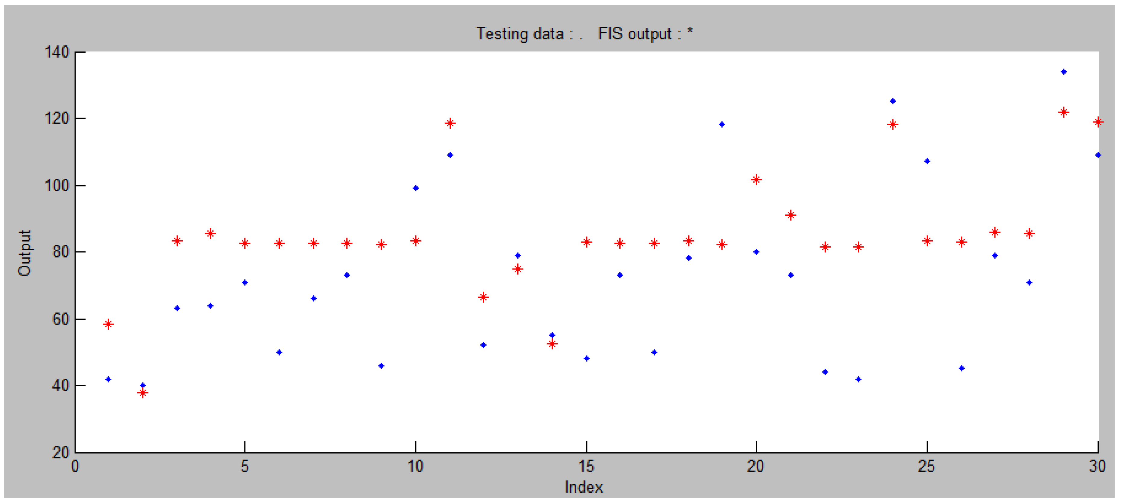
In addition to the tabular overview, the accuracy of the prediction can also be shown graphically, as in Figure 9. Red asterisks denote the outputs of the ANFIS model, while blue points denote measured checking data. The RMSE for such a set of data is 22.06. Although while testing the model it showed the least error of 13.67 over the testing data, the set of checking data is different from it, and that is the reason why, in this case, the RMSE has the given value.
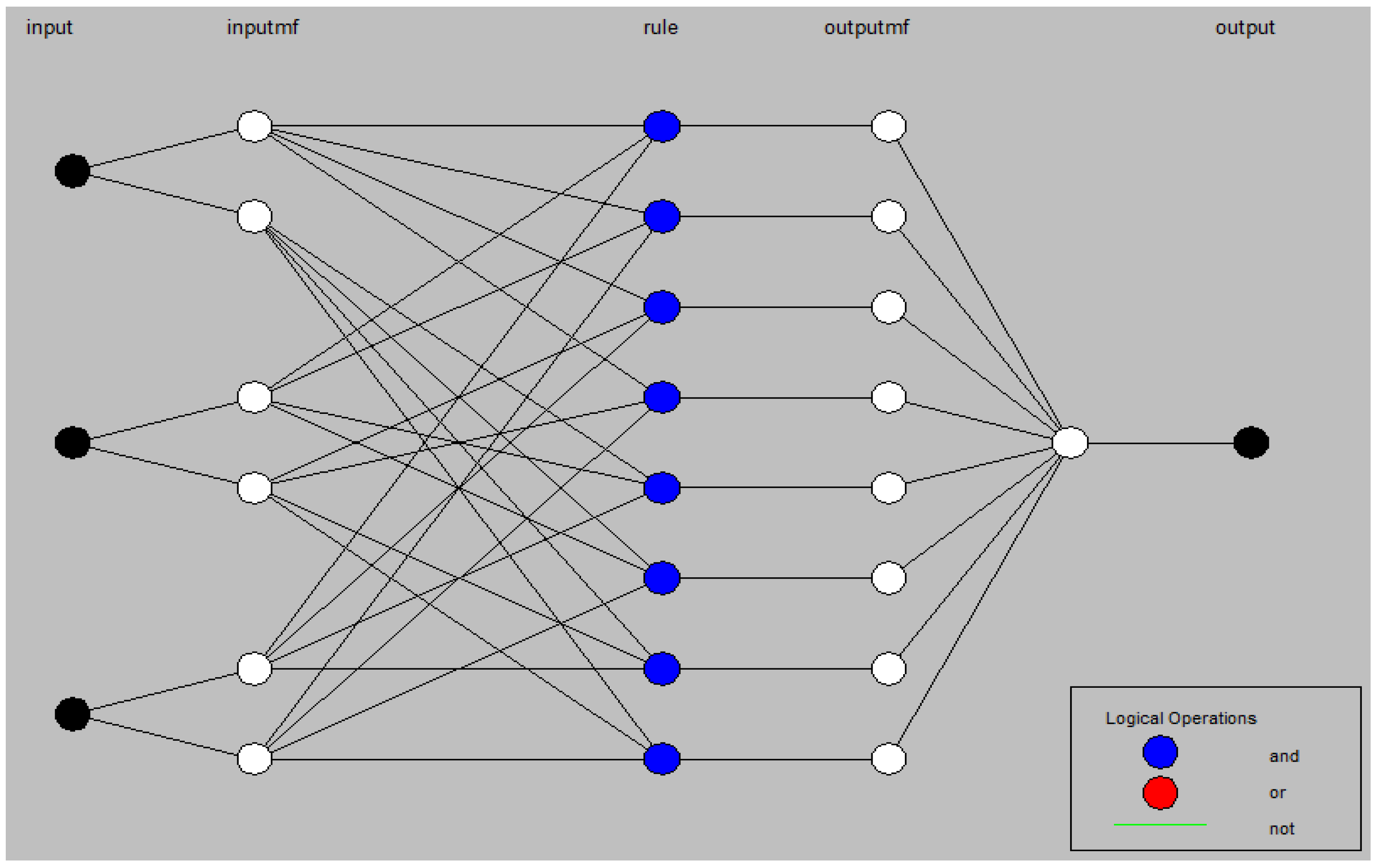
The structure of the selected model is shown in Figure 10, where the number of nodes in each layer of the neural network can be seen. It is obvious that in all fuzzy inference rules, of which there are 8 (the number of nodes in the third layer), the logical operator (AND) figures.
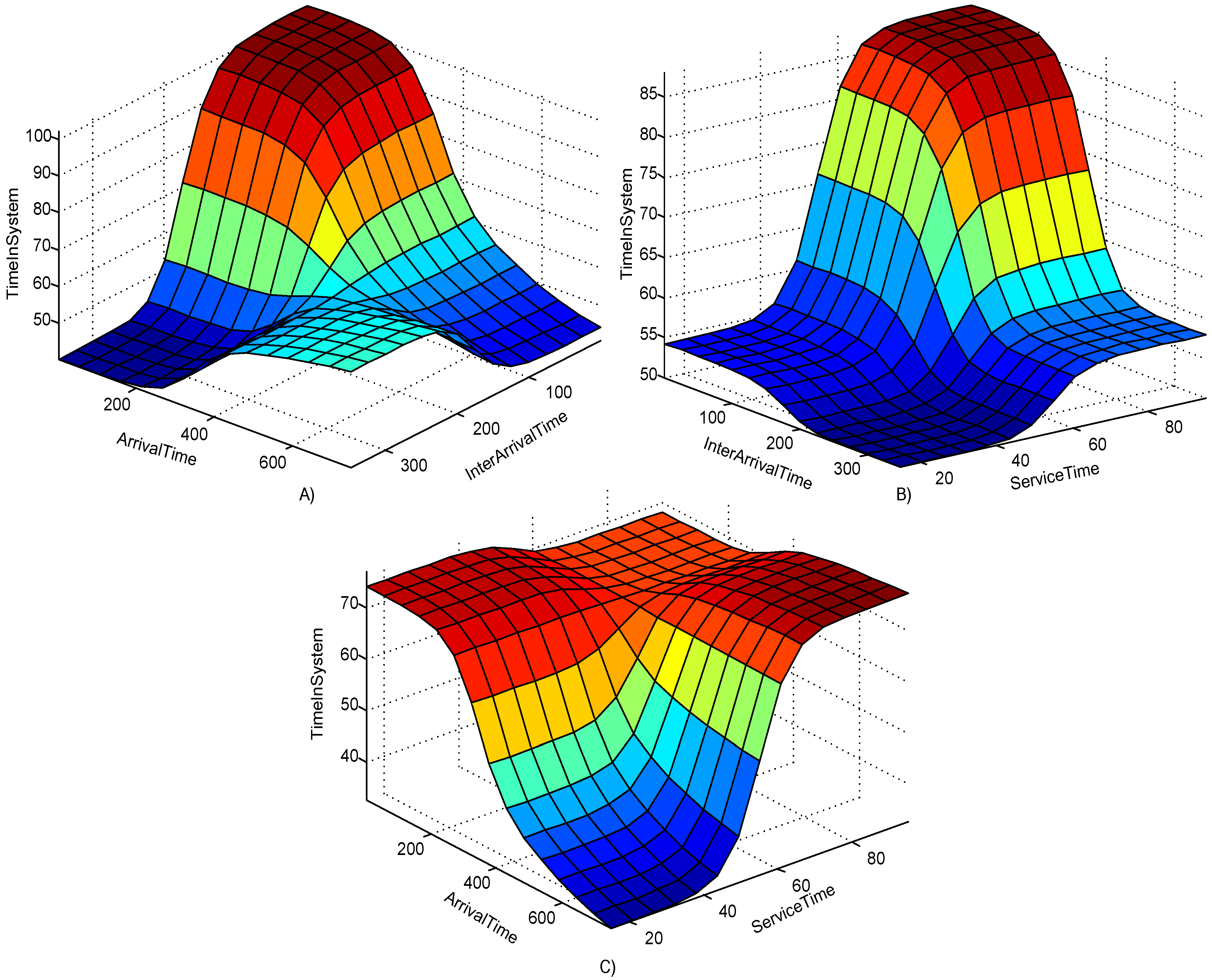
Figure 11 shows the surface of dependence, i.e. a portable function of the selected model. Taking into account that there are three input variables, the dependence of the output from the input is given for all three combinations. It is evident that the time spent in the system has a greater value in reducing inter-arrival times and the cumulative arrival time of trucks. Regarding the influence of the service time on the observed output, it is concluded that the time spent in the system increases with the increase of the specified variable and the decrease in inter-arrival times. An increase in the value of the output variable is also caused by an increase in the service time and simultaneous reduction in the cumulative arrival time.
6. Sensitivity Analysis
In order to validate the developed ANFIS model, it was compared with a mathematical model developed by regression analysis of training data. A polynomial mathematical model with the highest correlation index R2 = 15.58 was selected. The model is of the second degree and has the following form:
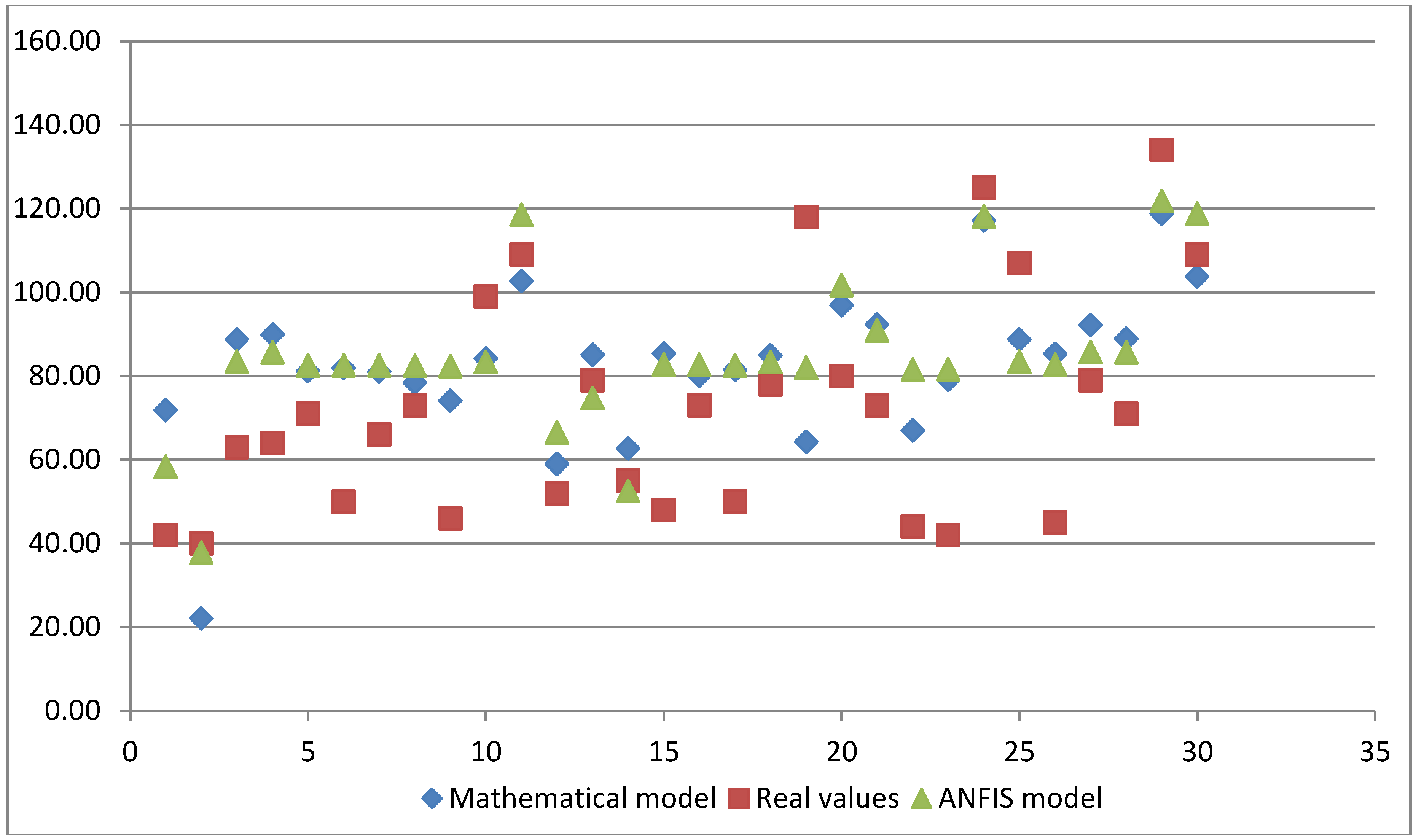
Table 8 gives an overview of the measured values of the time spent in the system and predicted values determined by the mathematical model and ANFIS for the same input data set. The RMSE value, in the case of the mathematical model, is 22.96, which means that the ANFIS model shows better performance.
Figure 12 gives a graphic display of the values shown in Table 8. The red squares represent the real or measured values of the time spent in the system. Blue rhombuses represent the predicted values obtained by the mathematical model of second degree, which is given by the expression (7). Predicted values obtained by the ANFIS model are marked with green triangles. The figure provides a visual performance analysis of the two models compared to the real values of the time spent in the system.
7. Conclusion
In this paper, a study on the modeling of a queuing system in a logistics company for the manufacturing of brown paper was conducted. An ANFIS model for modeling a time component of the system was developed as a criterion for optimization. The contributions of this research can be described in the following ways. The proposed neuro-fuzzy model extends the theoretical framework of knowledge in the field of QS. The QS problem is considered by a new methodology, and thus, a basis for further theoretical and practical upgrading is formed. In addition, the presented model emphasizes the unique practical parameters (the inter-arrival time of trucks, the cumulative time of arrival since an initial time, the service time), which, in former MSS models, have not been considered as unified, despite being of importance for this logistics company and its customers.
The proposed neuro-fuzzy model has four main advantages over other methods. First, in comparison with classical QS, it has an adaptability feature, which is reflected in its ability to adjust a fuzzy rule base. Fuzzy rules are very important for managing queuing systems, especially for a descriptive approach that prefers intuitive, heuristic searches of solutions in a queuing system process. This flexibility allows us to overcome the limitations of conventional QS models that perform a prediction of the flow throughout statistical consideration of parameters without intuitiveness. Second, the neuro-fuzzy model is effective under conditions of uncertainty, and can provide support to decision-makers when there is uncertainty in logistics processes. Third, it can be implemented as a computer system that supports a dynamic decision-making process in the QS. And fourth, the proposed model allows relatively fast and objective estimates to be made of serving the vehicles in a transportation company, under conditions of a changing environment. The continuation of this research may also include the optimization of other, smaller queuing systems for the decentralized storage system of this company.
Author Contributions
Each author has participated and contributed sufficiently to take public responsibility for appropriate portions of the content.
Conflicts of Interest
The authors declare no conflicts of interest.
References
- Stević, Ž.; Pamučar, D.; Kazimieras Zavadskas, E.; Ćirović, G.; Prentkovskis, O. The selection of wagons for the internal transport of a logistics company: A novel approach based on rough BWM and rough SAW methods. Symmetry 2017, 9, 264. [Google Scholar] [CrossRef]
- Stević, Ž.; Pamučar, D.; Vasiljević, M.; Stojić, G.; Korica, S. Novel Integrated multi-criteria model for supplier selection: Case study construction company. Symmetry 2017, 9, 279. [Google Scholar] [CrossRef]
- Stević, Ž.; Mulalić, E.; Božičković, Z.; Vesković, S.; Đalić, I. Economic analysis of the project of warehouse centralization in the paper production company. Serbian J. Manag. 2018, 13, 47–62. [Google Scholar] [CrossRef]
- Guerrouahane, N.; Aissani, D.; Bouallouche-Medjkoune, L.; Farhi, N. M/g/c/c state dependent queueing model for road traffic simulation. arXiv, 2016; arXiv:1612.09532. [Google Scholar]
- Raheja, T. Modelling traffic congestion using queuing networks. Sadhana 2010, 35, 427–431. [Google Scholar] [CrossRef]
- Van Woensel, T.; Vandaele, N. Queueing models for uninterrupted traffic flows. In Proceedings of the 13th Mini-EURO Conference Handling Uncertainty in the Analysis of Traffic and Transportation Systems, Bari, Italy, 2002; pp. 636–640. [Google Scholar]
- Vandaele, N.; Van Woensel, T.; Verbruggen, A. A queueing based traffic flow model. Transport. Res. D-Tr. E. 2000, 5, 121–135. [Google Scholar] [CrossRef]
- Osorio, C.; Bierlaire, M. Network performance optimization using a queueing network model. In Proceedings of the European Transport Conference, Langelaan, The Netherlands, 6–8 October 2008. [Google Scholar]
- Anokye, M.; Abdul-Aziz, A.R.; Annin, K.; Oduro, F.T. Application of queuing theory to vehicular traffic at signalized intersection in Kumasi-Ashanti region, Ghana. Am. Int. J. Cont. Res. 2013, 3, 23–29. [Google Scholar]
- Wang, F.; Ye, C.; Zhang, Y.; Li, Y. Simulation analysis and improvement of the vehicle queuing system on intersections based on MATLAB. Open Cybernet. Syst. J. 2014, 8, 217–223. [Google Scholar] [CrossRef]
- Chen, W.N. Application of queuing theory to dynamic vehicle routing problem. Glob. J. Bus. Res. 2009, 3, 85–91. [Google Scholar]
- Azizi, A.; Yarmohammadi, Y.; Yasini, A.; Sadeghifard, A. A queuing model to reduce energy consumption and pollutants production through transportation vehicles in green supply chain management. J. Sci. Res. Rep. 2015, 5, 571–581. [Google Scholar] [CrossRef]
- Aziziankohan, A.; Jolai, F.; Khalilzadeh, M.; Soltani, R.; Tavakkoli-Moghaddam, R. Green supply chain management using the queuing theory to handle congestion and reduce energy consumption and emissions from supply chain transportation fleet. J. Ind. Eng. Manag. 2017, 10, 213–236. [Google Scholar] [CrossRef]
- Gong, Y.; De Koster, R.B. A review on stochastic models and analysis of warehouse operations. Log. Res. 2011, 3, 191–205. [Google Scholar] [CrossRef]
- Masek, J.; Camaj, J.; Nedeliakova, E. Application the queuing theory in the warehouse optimization. Int. J. Soc. Behav. Educ. Econ. Bus. Ind. Eng. 2015, 9, 3744–3748. [Google Scholar]
- Cai, X.; Heragu, S.S.; Liu, Y. Modeling automated warehouses using semi-open queueing networks. In Handbook of Stochastic Models and Analysis of Manufacturing System Operations; Smith, J.M., Tan, B., Eds.; Springer-Verlag: New York, NY, USA, 2013; pp. 29–71. [Google Scholar]
- Bao-ping, C.; Zeng-Qiang, M. Short-term traffic flow prediction based on ANFIS. In Proceedings of the International Conference on Communication Software and Networks, Sichuan, China, 27–28 February 2009; pp. 791–793. [Google Scholar]
- Rahimi, A.M. Neuro-fuzzy system modelling for the effects of intelligent transportation on road accident fatalities. Tehnički Vjesn. 2017, 24, 1165–1171. [Google Scholar]
- Hosseinlou, M.H.; Sohrabi, M. Predicting and identifying traffic hot spots applying neuro-fuzzy systems in intercity roads. Int. J. Environ. Sci. Technol. 2009, 6, 309–314. [Google Scholar] [CrossRef] [Green Version]
- Suraj, S.; Jagrut, G. Smart traffic control using adaptive neuro-fuzzy Inference system (ANFIS). Int. J. Adv. Eng. Res. Dev. 2015, 2, 295–302. [Google Scholar]
- Araghi, S.; Khosravi, A.; Creighton, D. ANFIS traffic signal controller for an isolated intersection. In Proceedings of the International Conference on Fuzzy Computation Theory and Applications, Rome, Italy, 22–24 October 2014; pp. 175–180. [Google Scholar]
- Udofia, K.M.; Emagbetere, J.O.; Edeko, F.O. Dynamic traffic signal phase sequencing for an isolated intersection using ANFIS. Auto. Control Intell. Syst. 2014, 2, 21–26. [Google Scholar]
- Sharma, A.; Vijay, R.; Bodhe, G.L.; Malik, L.G. Adoptive neuro-fuzzy inference system for traffic noise prediction. Int. J. Comput. Appl. 2014, 98, 14–19. [Google Scholar] [CrossRef]
- Pamučar, D.; Ćirović, G. Vehicle route selection with an adaptive neuro fuzzy inference system in uncertainty conditions. Decis. Mak. Appl. Manag. Eng. 2018, 1, 13–37. [Google Scholar] [CrossRef]
- Andrade, K.; Uchida, K.; Kagaya, S. Development of transport mode choice model by using adaptive neuro-fuzzy inference system. Transport. Res. Rec.-J. Transport. Res. Board 2006, 1977, 8–16. [Google Scholar] [CrossRef]
- Mircetic, D.; Lalwani, C.; Lirn, T.; Maslaric, M.; Nikolicic, S. ANFIS expert system for cargo loading as part of decision support system in warehouse. In Proceedings of the 19th International Symposium on Logistics (ISL 2014), Ho Chi Minh City, Vietnam, 6–9 July 2014; pp. 10–20. [Google Scholar]
- Mirčetić, D.; Ralević, N.; Nikoličić, S.; Maslarić, M.; Stojanović, Đ. Expert system models for forecasting forklifts engagement in a warehouse loading operation: A case study. PROMET-Zagreb. 2016, 28, 393–401. [Google Scholar] [CrossRef]
- Marto, M.; Reynolds, K.; Borges, J.; Bushenkov, V.; Marques, S. Combining Decision Support Approaches for Optimizing the Selection of Bundles of Ecosystem Services. Forests 2018, 9, 438. [Google Scholar] [CrossRef]
- Al-Anbari, M.A.; Thameer, M.Y.; Al-Ansari, N. Landfill Site Selection by Weighted Overlay Technique: Case Study of Al-Kufa, Iraq. Sustainability 2018, 10, 999. [Google Scholar] [CrossRef]
- Sałabun, W.; Karczmarczyk, A. Using the COMET Method in the Sustainable City Transport Problem: An Empirical Study of the Electric Powered Cars. Procedia Comput. Sci. 2018, 126, 2248–2260. [Google Scholar] [CrossRef]
- Wątróbski, J.; Sałabun, W.; Karczmarczyk, A.; Wolski, W. Sustainable decision-making using the COMET method: An empirical study of the ammonium nitrate transport management. In Proceedings of the 2017 Federated Conference on Computer Science and Information Systems, Prague, Czech Republic, 3–6 September 2017; pp. 949–958. [Google Scholar]
- Wątróbski, J.; Sałabun, W.; Ladorucki, G. The temporal supplier evaluation model based on multicriteria decision analysis methods. In Proceedings of the Asian Conference on Intelligent Information and Database Systems, Kanazawa, Japan, 3–5 April 2017; pp. 432–442. [Google Scholar]
- Khalili-Damghani, K.; Dideh-Khani, H.; Sadi-Nezhad, S. A two-stage approach based on ANFIS and fuzzy goal programming for supplier selection. Int. J. Appl. Decis. Sci. 2013, 6, 1–14. [Google Scholar]
- Torkabadi, A.M.; Mayorga, R.V. Optimization of Supply Chain based on JIT Pull Control Policies: An Integrated Fuzzy AHP and ANFIS Approach. WSEAS Trans. Comput. 2017, 16, 366–377. [Google Scholar]
- Pirdavani, A.; Brijs, T.; Wets, G. A Multiple Criteria Decision-Making Approach for Prioritizing Accident Hotspots in the Absence of Crash Data. Transp. Rev. 2010, 30, 97–113. [Google Scholar] [CrossRef]
- Stević, Ž.; Pamučar, D.; Subotić, M.; Antuchevičiene, J.; Zavadskas, E. The Location Selection for Roundabout Construction Using Rough BWM-Rough WASPAS Approach Based on a New Rough Hamy Aggregator. Sustainability 2018, 10, 2817. [Google Scholar] [CrossRef]
- Stidham, S., Jr. Analysis, design, and control of queueing systems. Oper. Res. 2002, 50, 197–216. [Google Scholar] [CrossRef]
- Cooper, R.B. Introduction to queueing theory, 2nd ed.; Fineman, J., Schreiber, L.C., Eds.; North Holland: New York, NY, USA, 1981. [Google Scholar]
- Maragatha, S.; Srinivasan, S. Analysis of M/M/I queueing model for ATM facility. Glob. J. Theor.Appl. Mathematics Sci. 2012, 2, 41–46. [Google Scholar]
- Defraeye, M.; Van Nieuwenhuyse, I. Staffing and scheduling under nonstationary demand for service: A literature review. Omega 2016, 58, 4–25. [Google Scholar] [CrossRef]
- Stević, Ž. Calculation of the basic parameters of queuing systems using winqsb software. In Proceedings of the XI International May Conference on Strategic Management, Bor, Serbia, 29–31 May 2015; pp. 91–100. [Google Scholar]
- Sremac, S.; Tanackov, I.; Kopić, M.; Radović, D. ANFIS model for determining the economic order quantity. Decis. Mak. Appl. Manag. Eng. 2018, 1, 1–12. [Google Scholar] [CrossRef]
- Tiwari, S.; Babbar, R.; Kaur, G. Performance evaluation of two ANFIS models for predicting water quality Index of River Satluj (India). Adv. in Civ. Eng. 2018, 2018, 1–10. [Google Scholar] [CrossRef]
- Billah, M.; Waheed, S.; Ahmed, K.; Hanifa, A. Real time traffic sign detection and recognition using adaptive neuro fuzzy inference system. Commun. Appl. Electron. 2015, 3, 1–5. [Google Scholar] [CrossRef]
- Qasem, S.N.; Ebtehaj, I.; Riahi Madavar, H. Optimizing ANFIS for sediment transport in open channels using different evolutionary algorithms. J. Appl. Res. Water Wastewater 2017, 4, 290–298. [Google Scholar]
- Lukovac, V.; Pamučar, D.; Popović, M.; Đorović, B. Portfolio model for analyzing human resources: An approach based on neuro-fuzzy modeling and the simulated annealing algorithm. Expert Syst. Appl. 2017, 90, 318–331. [Google Scholar] [CrossRef]
- Pamučar, D.; Ljubojević, S.; Kostadinović, D.; Đorović, B. Cost and risk aggregation in multi-objective route planning for hazardous materials transportation—A neuro-fuzzy and artificial bee colony approach. Expert Syst. Appl. 2016, 65, 1–15. [Google Scholar] [CrossRef]
- Das, R.D.; Winter, S. Detecting urban transport modes using a hybrid knowledge driven framework from GPS trajectory. ISPRS Int. J. Geo-Inf. 2016, 5, 207. [Google Scholar] [CrossRef]
- Engmann, S.; Cousineau, D. Comparing distributions: The two-sample Anderson-Darling test as an alternative to the Kolmogorov-Smirnoff test. J. Appl. Quant. Methods 2011, 6, 1–17. [Google Scholar]
- Stephens, M.A. Tests based on EDF statistics. In Goodness of Fit. Techniques Chapter 4; D’Agostino, R.B., Stephens, M.A., Eds.; Routledge: New York, NY, USA, 1986. [Google Scholar]
- Barford, P.; Crovella, M. Generating representative web workloads for network and server performance evaluation. In ACM SIGMETRICS Performance Evaluation Review; ACM: New York, NY, USA, 1998; pp. 151–160. [Google Scholar]
- Jovanović, B.; Grbić, T.; Bojović, N.; Kujačić, M.; Šarac, D. Application of ANFIS for the Estimation of Queuing in a Postal Network Unit: A Case Study. Acta Polytech. Hung. 2015, 12, 25–40. [Google Scholar]
Figure 1.
Diagram of the research flow.

Figure 2.
The ANFIS structure with two inputs.

Figure 3.
The basic process of the queuing system for the PM4 warehouse4.1. Data collection.

Figure 4.
Time in the system and cumulative arrival time for 237 trucks.

Figure 5.
Poisson distribution of the input flow.

Figure 6.
Distribution of the service time.

Figure 7.
Steps of the process from creation to testing of the ANFIS model.

Figure 8.
Fuzzy functions of membership for the input variable of inter-arrival time.

Figure 9.
Deviations of the ANFIS model output from the measured testing data.

Figure 10.
The structure of the selected ANFIS model.

Figure 11.
The surface of the dependence of the time spent in the system from: (a) inter-arrival time and arrival time; (b) inter-arrival time and service time; (c) arrival time and service time.
Figure 11.
The surface of the dependence of the time spent in the system from: (a) inter-arrival time and arrival time; (b) inter-arrival time and service time; (c) arrival time and service time.

Figure 12.
Values obtained by the mathematical and ANFIS model and the actual measured ones.


Table 1.
Frequencies of the input flow for a period of one hour.
| Number of Trucks | Frequency |
|---|---|
| 0 | 214 |
| 1 | 48 |
| 2 | 46 |
| 3 | 14 |
| 4 | 8 |
| 5 | 2 |
Table 2.
The results of statistical tests for determining the fitting of the input flow to a certain distribution.
Table 2.
The results of statistical tests for determining the fitting of the input flow to a certain distribution.
| Distribution | Anderson Darling | |
|---|---|---|
| Statistic | Rank | |
| Poisson | 88.26 | 1 |
| Geometric | 112.79 | 2 |
| D. Uniform | 197.01 | 3 |
| Bernoulli | No fit (data max > 1) | |
| Binomial | No fit | |
| Hyper-geometric | No fit | |
| Logarithmic | No fit (data min < 1) | |
| Neg. Binomial | No fit | |
Table 3.
Frequencies of the service time.
| Class Limits | Arithmetic Mean of Class-Interval | Frequency (Number of Trucks) |
|---|---|---|
| 15–25 | 20 | 46 |
| 26–36 | 31 | 72 |
| 37–47 | 42 | 68 |
| 48–58 | 53 | 22 |
| 59–69 | 64 | 6 |
| 70–80 | 75 | 0 |
| 81–91 | 83 | 6 |
| 92–102 | 97 | 4 |
Table 4.
Results of statistical tests for determining the fitting of service times to a certain distribution.
Table 4.
Results of statistical tests for determining the fitting of service times to a certain distribution.
| Distribution | Anderson Darling | |
|---|---|---|
| Statistic | Rank | |
| Levy | 1.5611 | 1 |
| Levy (2P) | 1.6041 | 2 |
| Pareto 2 | 2.3671 | 3 |
| Exponential | 2.9128 | 4 |
| Rayleigh | 3.6386 | 5 |
| Reciprocal | 3.8271 | 6 |
| Log-Logistic (3P) | 4.2251 | 7 |
| Fatigue Life (3P) | 4.4674 | 8 |
Table 5.
The values of average testing errors of different ANFIS models with constant output.
| Shape of Fuzzy Membership Functions | Number of Fuzzy Membership Functions for Each of Three Input Variables | |||||||
|---|---|---|---|---|---|---|---|---|
| 2 2 2 | 3 3 3 | 2 2 3 | 2 3 2 | 2 3 3 | 3 3 2 | 3 2 3 | 3 2 2 | |
| Trimf | 18.66 | 64.64 | 21.53 | 22.94 | 30.46 | 66.73 | 23.30 | 20.72 |
| Trapmf | 14.23 | 27.72 | 16.16 | 14.33 | 16.64 | 16.46 | 20.55 | 18.11 |
| Gbellmf | 19.46 | 47.00 | 19.66 | 21.42 | 58.65 | 17.34 | 46.14 | 16.29 |
| Gaussmf | 16.91 | 307.84 | 20.26 | 17.81 | 26.91 | 31.49 | 22.64 | 17.79 |
| Gauss2mf | 14.30 | 20.50 | 63.56 | 15.70 | 22.40 | 26.89 | 19.16 | 17.83 |
| Pimf | 14.78 | 23.21 | 17.10 | 14.05 | 17.19 | 15.07 | 21.25 | 17.42 |
| Dsigmf | 13.67 | 64.43 | 24.38 | 17.09 | 60.50 | 28.00 | 19.29 | 17.46 |
| Psigmf | 13.67 | 64.43 | 24.38 | 17.09 | 60.50 | 28.00 | 19.29 | 17.46 |
Table 6.
The values of average testing errors of different ANFIS models with linear output.
| Shape of Fuzzy Membership Functions | Number of Fuzzy Membership Functions for Each of Three Input Variables | |||||||
|---|---|---|---|---|---|---|---|---|
| 2 2 2 | 3 3 3 | 2 2 3 | 2 3 2 | 2 3 3 | 3 3 2 | 3 2 3 | 3 2 2 | |
| Trimf | 217.63 | 13557.47 | 577.56 | 836.02 | 1726.74 | 35925.48 | 19459.66 | 1219.73 |
| Trapmf | 116.57 | 318.80 | 219.14 | 38.82 | 25.42 | 60.76 | 294.55 | 44.87 |
| Gbellmf | 22.19 | 34006.56 | 187.06 | 5305.95 | 23183.85 | 14176.49 | 50418.31 | 6937.78 |
| Gaussmf | 33.02 | 24328.30 | 257.99 | 3293.97 | 11566.52 | 5466.29 | 51114.92 | 108.12 |
| Gauss2mf | 253.78 | 3727.55 | 319.52 | 9477.00 | 34019.82 | 3765.83 | 14012.94 | 2537.84 |
| Pimf | 841.49 | 597.19 | 2104.52 | 222.63 | 23.77 | 44.86 | 415.37 | 190.11 |
| Dsigmf | 588.50 | 4961.53 | 2289.36 | 774.68 | 65680.67 | 2563.84 | 19890.09 | 449.44 |
| Psigmf | 427.85 | 5027.61 | 1118.50 | 1120.38 | 62986.63 | 7788.29 | 15398.09 | 4170.70 |
Table 7.
The values of the prediction of the time spent in the system and checking data.
| Ordinal Number | Checking Data | ANFIS Output | |||
|---|---|---|---|---|---|
| Inter-Arrival Interval | Arrival Time | Service Time | Time Spent in the System | ||
| 1st | 2 | 357 | 30 | 42 | 58.36 |
| 2nd | 272 | 629 | 25 | 40 | 37.84 |
| 3rd | 1 | 1 | 40 | 63 | 83.49 |
| 4th | 24 | 25 | 45 | 64 | 85.68 |
| 5th | 8 | 33 | 30 | 71 | 82.53 |
| 6th | 1 | 1 | 30 | 50 | 82.54 |
| 7th | 11 | 12 | 30 | 66 | 82.54 |
| 8th | 2 | 14 | 25 | 73 | 82.47 |
| 9th | 77 | 91 | 30 | 46 | 82.34 |
| 10th | 40 | 109 | 40 | 99 | 83.34 |
| 11th | 20 | 129 | 65 | 109 | 118.59 |
| 12th | 170 | 299 | 30 | 52 | 66.57 |
| 13th | 1 | 300 | 45 | 79 | 74.73 |
| 14th | 83 | 383 | 30 | 55 | 52.54 |
| 15th | 1 | 1 | 35 | 48 | 82.77 |
| 16th | 54 | 55 | 35 | 73 | 82.70 |
| 17th | 3 | 58 | 30 | 50 | 82.51 |
| 18th | 35 | 93 | 40 | 78 | 83.39 |
| 19th | 60 | 153 | 15 | 118 | 82.03 |
| 20th | 3 | 156 | 55 | 80 | 101.73 |
| 21st | 12 | 168 | 50 | 73 | 90.92 |
| 22nd | 21 | 189 | 15 | 44 | 81.54 |
| 23rd | 1 | 190 | 30 | 42 | 81.62 |
| 24th | 50 | 240 | 95 | 125 | 118.06 |
| 25th | 1 | 1 | 40 | 107 | 83.49 |
| 26th | 2 | 3 | 35 | 45 | 82.77 |
| 27th | 1 | 4 | 45 | 79 | 85.69 |
| 28th | 34 | 38 | 45 | 71 | 85.66 |
| 29th | 7 | 45 | 85 | 134 | 121.85 |
| 30th | 20 | 65 | 65 | 109 | 118.79 |
Table 8.
Measured values of time in the system and predicted values determined by the mathematical and ANFIS model.
Table 8.
Measured values of time in the system and predicted values determined by the mathematical and ANFIS model.
| Measured, Real Values | Mathematical Model | ANFIS Model |
|---|---|---|
| 42 | 71.84 | 58.36 |
| 40 | 22.03 | 37.84 |
| 63 | 88.75 | 83.49 |
| 64 | 89.95 | 85.68 |
| 71 | 81.17 | 82.53 |
| 50 | 81.92 | 82.54 |
| 66 | 80.96 | 82.54 |
| 73 | 78.39 | 82.47 |
| 46 | 74.12 | 82.34 |
| 99 | 84.15 | 83.34 |
| 109 | 102.73 | 118.59 |
| 52 | 59.03 | 66.57 |
| 79 | 85.11 | 74.73 |
| 55 | 62.72 | 52.54 |
| 48 | 85.33 | 82.77 |
| 73 | 80.11 | 82.70 |
| 50 | 81.46 | 82.51 |
| 78 | 84.87 | 83.39 |
| 118 | 64.29 | 82.03 |
| 80 | 96.90 | 101.73 |
| 73 | 92.33 | 90.92 |
| 44 | 66.99 | 81.54 |
| 42 | 79.09 | 81.62 |
| 125 | 117.19 | 118.06 |
| 107 | 88.75 | 83.49 |
| 45 | 85.24 | 82.77 |
| 79 | 92.16 | 85.69 |
| 71 | 88.95 | 85.66 |
| 134 | 118.76 | 121.85 |
| 109 | 103.70 | 118.79 |
© 2018 by the authors. Licensee MDPI, Basel, Switzerland. This article is an open access article distributed under the terms and conditions of the Creative Commons Attribution (CC BY) license (http://creativecommons.org/licenses/by/4.0/).
Share and Cite
MDPI and ACS Style
Stojčić, M.; Pamučar, D.; Mahmutagić, E.; Stević, Ž. Development of an ANFIS Model for the Optimization of a Queuing System in Warehouses. Information 2018, 9, 240. https://0-doi-org.brum.beds.ac.uk/10.3390/info9100240
AMA Style
Stojčić M, Pamučar D, Mahmutagić E, Stević Ž. Development of an ANFIS Model for the Optimization of a Queuing System in Warehouses. Information. 2018; 9(10):240. https://0-doi-org.brum.beds.ac.uk/10.3390/info9100240
Chicago/Turabian StyleStojčić, Mirko, Dragan Pamučar, Eldina Mahmutagić, and Željko Stević. 2018. "Development of an ANFIS Model for the Optimization of a Queuing System in Warehouses" Information 9, no. 10: 240. https://0-doi-org.brum.beds.ac.uk/10.3390/info9100240
Note that from the first issue of 2016, this journal uses article numbers instead of page numbers. See further details here.