Article

Limits of Compartmental Models and New Opportunities for Machine Learning: A Case Study to Forecast the Second Wave of COVID-19 Hospitalizations in Lombardy, Italy

by
Andrea Gatto
1,2,†,
Gabriele Accarino
1,3,†,
Valeria Aloisi
1,2,†,
Francesco Immorlano
1,2,
Francesco Donato
4 and
Giovanni Aloisio
1,2,*
1
Euro-Mediterranean Center on Climate Change (CMCC) Foundation, Via Augusto Imperatore, 16, 73100 Lecce, Italy
2
Department of Innovation Engineering, University of Salento, Via Provinciale Lecce-Monteroni, 73100 Lecce, Italy
3
Department of Biological and Environmental Sciences and Technologies, University of Salento, Via Provinciale Lecce-Monteroni, 73100 Lecce, Italy
4
Unit of Hygiene, Epidemiology, and Public Health, Department of Medical and Surgical Specialties, Radiological Sciences and Public Health, University of Brescia, Viale Europa 11, 25123 Brescia, Italy
*
Author to whom correspondence should be addressed.
These authors contributed equally to this work.
Submission received: 21 July 2021 / Revised: 18 August 2021 / Accepted: 27 August 2021 / Published: 31 August 2021
(This article belongs to the Section Health Informatics)

Abstract

:
Compartmental models have long been used in epidemiological studies for predicting disease spread. However, a major issue when using compartmental mathematical models concerns the time-invariant formulation of hyper-parameters that prevent the model from following the evolution over time of the epidemiological phenomenon under investigation. In order to cope with this problem, the present work suggests an alternative hybrid approach based on Machine Learning that avoids recalculation of hyper-parameters and only uses an initial set. This study shows that the proposed hybrid approach makes it possible to correct the expected loss of accuracy observed in the compartmental model when the considered time horizon increases. As a case study, a basic compartmental model has been designed and tested to forecast COVID-19 hospitalizations during the first and the second pandemic waves in Lombardy, Italy. The model is based on an extended formulation of the contact function that allows modelling of the trend of personal contacts throughout the reference period. Moreover, the scenario analysis proposed in this work can help policy-makers select the most appropriate containment measures to reduce hospitalizations and relieve pressure on the health system, but also to limit any negative impact on the economic and social systems.

1. Introduction

In early December 2019, the first COronaVIrus Disease-2019 (COVID-19) case was identified in Wuhan, China [1], which started a pandemic that spread across the globe in just a few months [2]. COVID-19 is a disease caused by a new form of coronavirus named Severe Acute Respiratory Syndrome CoronaVirus type 2 (SARS-CoV-2) [1,3]. The most common symptoms are fever, fatigue, and dry cough, which can evolve, in severe cases, into pneumonia, severe acute respiratory syndrome, and death [4]. The disease has been spreading fast and more than 65 million people have been infected as of fifth December 2020, with more than 1.5 million deaths around the world [2]. In Italy, the first COVID-19 case was announced on 20 February 2020 in Codogno, Lombardy [5]. In a few days, the contagion started spreading throughout the country and, for this reason, the Italian government announced a national lockdown on 9 March 2020 to contain the virus [6]. The lockdown period ended on 4 May 2020, but the circulation of the virus has never really stopped in Italy, with few cases in Summer, but a rapid increase of the pandemic spread since September reaching a total of about 1.7 million cumulative cases on 6 December [7]. According to scientific literature, compartmental mathematical models have been widely used to emulate the behavior of infectious diseases and to map specific phenomenon-based characteristics within the model. Compartmental models were first introduced by Kermack and McKendrick [8] in 1991 with the Susceptible, Infected, and Recovered (SIR) formulation [9]. Several other studies using compartmental models have also been published, especially aimed at modelling COVID-19 spread in different countries by focusing on multiple variables. In particular, Chen and colleagues [10] developed a multilevel transmission network (called BHRP: bats, host, reservoir, people) based on the Susceptible, Exposed, Infected and Recovered (SEIR) paradigm in order to emulate COVID-19 transmission in China. Starting from the initial outbreak among bats, the method by Runge-Kutta [11] was adopted to estimate the model equations hyper-parameters based on Chinese official data. Moreover, an age-structured SEIR model was proposed by Prem and colleagues [12] to evaluate the effect of social distancing measures on the outcomes of the COVID-19 epidemic in Wuhan, China. Kucharski and colleagues [13] conducted a mathematical study based on a stochastic SEIR model, with the goal of modelling the early dynamics of COVID-19 pandemic transmission in Wuhan, also considering the impact of travelling on the virus spread outside Wuhan. A modified SEIR model was used by Yang and colleagues [14] to derive the COVID-19 epidemic curve in China. A Machine Learning approach, trained on the 2003 SARS data, was also used to predict the epidemic spread. An Extended SEIR model was proposed by Tang and colleagues [15,16] to predict the trend of COVID-19 hospitalizations in China, which included some time-variant hyper-parameters to implement a dynamic setting of the model. The same model was used for the Italian case [17] to forecast COVID-19 related variables in two Italian regions. Bollon and colleagues [18] used compartmental mathematical models to assess the role of containment measures in curbing the demand for hospitalization. Rǎdulescu and colleagues [19] adapted a traditional SEIR model based on four age groups to analyze the effect of containment measures strategies in USA. Moreover, Giordano and colleagues [20] developed a new mathematical model based on eight compartments to forecast COVID-19 trend in Italy. Ahmad and colleagues [21] proposed a fractional SEIR model to investigate the spread of the COVID-19 in Pakistan during the first pandemic wave using, also, the next generation matrix algorithm to compute the basic reproduction number R 0 . Kuzdeuov and colleagues [22] developed a COVID-19 simulator for Kazakhistan through a stochastic SEIR model. The simulator exploits a variety of data such as epidemiological, population demographics and mobility. Moreover, Gaglione and colleagues [23] used a Bayesian sequential and adaptive dynamic estimation method for computing the infection and recovery parameters, and to track and predict the epidemiological curve in Lombardy, Italy, and in USA. A SEIR model has also been exploited by Bherwani and colleagues [24] to emulate the spread of the COVID-19 epidemic in India. Battineni et al. [25] also developed a SEIR model explaining the infection growth across Italy and presenting epidemic rates after and before country lockdown. A study related to the COVID-19 second wave in Italy has been proposed by Chintalapudi et al. [26] evaluating the basic reproduction number.
Moreover, Zisad et al. [27] proposed an integrated Neural Network and SEIR Model to predict COVID-19 spread in Bangladesh. Furthermore, Alanazi et al. [28] developed a framework based on SIR model and Machine Learning for measuring and preventing the continued spread of COVID-19 in the Kingdom of Saudi Arabia (KSA).
Growth models have been also used to understand COVID-19 epidemic outbreaks by Tovissodé et al. [29], as well as in [30] to fit the number of cumulative confirmed cases for revealing the patterns and the rate of COVID-19 spread in different countries. A second wave of the COVID-19 pandemic has started in Europe since the end of Summer, which achieved a peak in November [31]. However, all the mathematical models based on the first wave of the pandemic were not able to provide an accurate forecast of the second COVID-19 pandemic curve, mainly due to substantial parametric changes from the first to the second wave. In general, a major issue when using compartmental mathematical models relates to the gradual loss of accuracy coming from the time-invariant formulation of hyper-parameters, which actually prevent the model from following the evolution over time of the epidemiological phenomenon under investigation. Such hyper-parameters are generally calculated on the basis of appropriate estimation algorithms (e.g., MCMC, Maximum Likelihood) that do not provide time-variant formulations though. For this reason, each hyper-parameter should be defined with a time-variant formulation that would allow the model to adapt to the different boundary conditions observed throughout the evolution of the investigated phenomenon. The problem is exacerbated in the case of complex compartmental models like the model in this work, based on nine compartments and 29 hyper-parameters. In order to cope with this problem, the present work suggests an alternative approach, based on Machine Learning, that avoids recalculation of hyper-parameters and only uses an initial set. As the time frame increases, the expected loss of accuracy in the model is corrected through an approach based on machine learning. Indeed, in the present study, a Hybrid SEIR Model (from now on called HSM) framework, has been designed by coupling a Basic SEIR Model (from now on called BSM) and Machine Learning (ML), which led to a novel hybrid framework that takes advantage of both approaches. The developed HSM has been used here to produce accurate predictions about COVID-19 hospitalizations for the second epidemic wave, to simulate different scenarios based on different containment measures and to assess the impact of such measures on the epidemiological curve, using the HSM framework.

2. Materials and Methods

2.1. Population and Data Sources

To avoid model uncertainty due to inter-country and inter-regional variability, we restricted the application of the model to the Lombardy region, North Italy, which is one of the most affected regions in Italy and Europe, with more than 400,000 cases and 20,000 deaths in 10 million inhabitants on 6 December, with a cumulative incidence of about 4% [32]. The number of hospitalizations was chosen as the target variable because it reflects the number of severe cases and does not depend on the number of swabs, which has varied substantially over time in Italy. Keeping track of hospitalizations is strategic for policy-makers as it allows predicting the potential saturation of the hospital system, and when this might happen. Moreover, data concerning COVID-19 hospitalizations, deaths, isolated infected patients, infected patients, number of swabs and recovered patients in the period from 9 March to 6 January 2021 were collected from the Italian Civil Protection Department (ICPD) repository [33]. The average recovery period of hospitalized patients has been estimated to be equal to 14 days by the Regional Health Agency (ARS) of Tuscany, Italy [34]. This period corresponds to the worst case identified by ARS among the five trajectories related to hospitalization duration according to different severity scenarios. For the BSM modelling phase, other parameters regarding the COVID-19 epidemic spread have been collected from Tang and colleagues [15,16] as well as from Reno and colleagues [17].

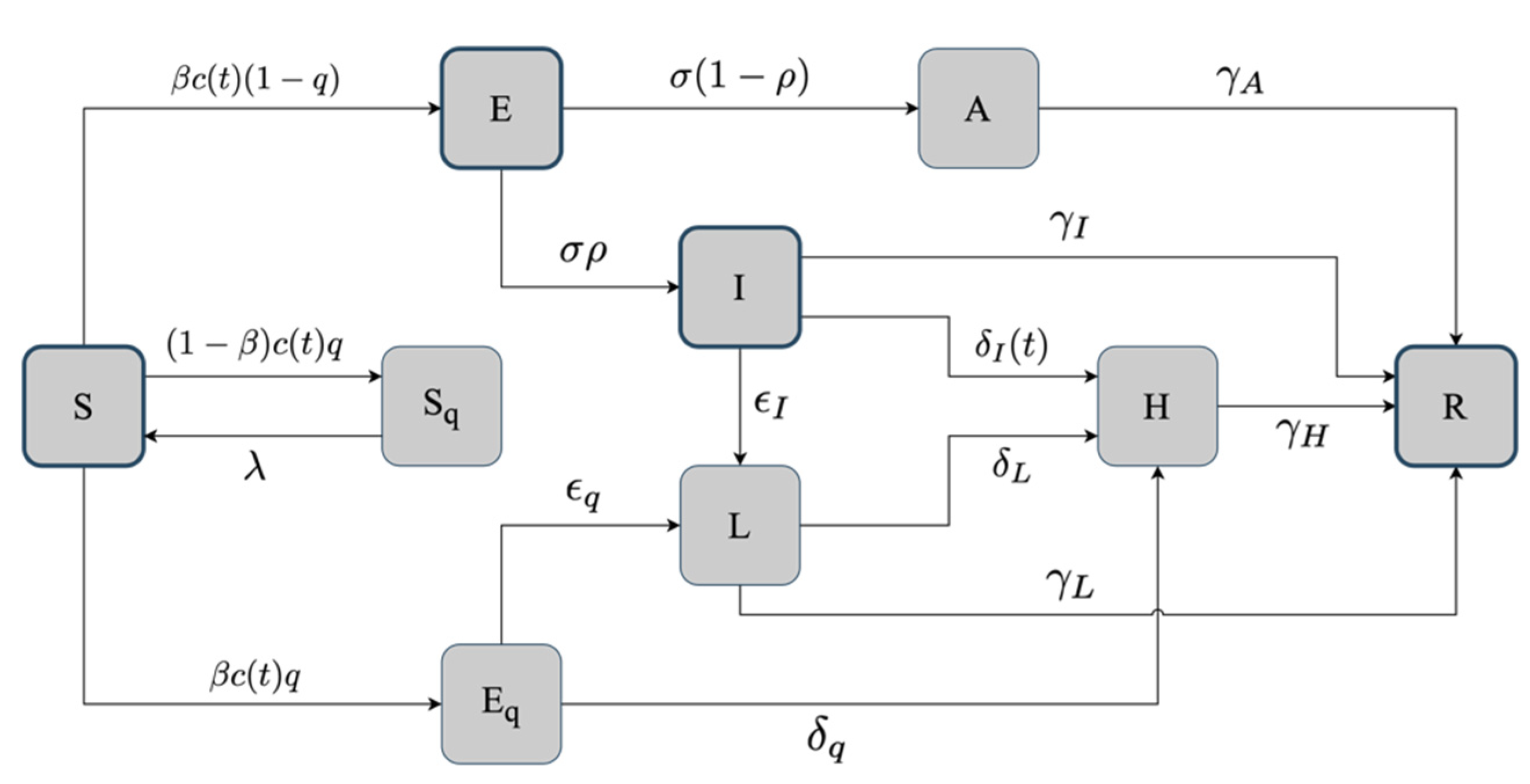
2.2. The Basic SEIR Model

The Basic SEIR Model (BSM) is a closed-population compartmental model. Based on the SEIR model first introduced by Tang and colleagues [15,16] and subsequently adapted by Reno and colleagues [17] to the Italian case, BSM has been proposed by redefining some hyper-parameters related to the underlying differential equations. As shown in Figure 1, BSM takes into account nine compartments.
Each compartment is connected to one or more compartments through directed segments, and their interaction is regulated by the rate associated with each segment. Formally, BSM is defined by the following system of ordinary differential equations that allows modelling important epidemiological characteristics related to the COVID-19 spread in Lombardy:
S = ( β c ( t ) + c ( t ) q ( 1 β ) ) S ( I + θ A ) + λ S q E = β c ( t ) ( 1 q ) S ( I + θ A ) σ E I = σ ρ E ( δ I ( t ) + ϵ I + γ I + α ) I A = σ ( 1 ρ ) E γ A A S q = ( 1 β ) c ( t ) q S ( I + θ A ) λ S q E q = β c ( t ) q S ( I + θ A ) ( δ q + ϵ q ) E q L = ϵ q E q + ϵ I I ( δ L + γ L + α ) L H = δ I ( t ) I + δ q E q + δ L L ( γ H + α ) H R = γ I I + γ A A + γ H H + γ L L
The solution of the system above is obtained by integrating differential equations over a time interval starting from a set of initial conditions, reported in Table A1 of Appendix A, and related to compartments. The time evolution of each compartment depends on a series of hyper-parameters whose values have been estimated based on the available data and information about the first pandemic wave. The full set of hyper-parameters is reported in Table A2 of Appendix A. Hyper-parameters play an important role in modelling region-specific outbreak dynamics, since the simulated trends strongly depend on the parameter’s choice. Most hyper-parameters values are those proposed by Tang and colleagues [16] as well as by Reno and colleagues [17] because some parallelism seems to exist between the outbreak dynamics observed in Lombardy (Italy) and in Wuhan (China), even though with different population characteristics. Further hyper-parameters have been added whereas others have been redefined in order to improve the BSM forecasting performance in Lombardy. As the virus is mainly transmitted through contact, the modeling of an appropriate “contact function” was necessary to allow for the impact of containment measures on the gradual trend in the number of contacts. Information about the contact rate was not available at the time of writing. Hence, an intuitive approach has been applied using mobility data provided by Apple [35], as better explained in Appendix A. Therefore, the contact rate c ( t ) has been defined as:
c ( t ) =   c w 1 ( t ) + c w 2 ( t )
where:
c w 1 ( t ) = 1 1 + e α 1 ( ( T L 2 + Δ T L 2 ) t )   [   1 1 + e α 1 ( L 1 t )   c 1 ( t ) + 1 1 + e α 2 ( t L 1 )   c 2 ( t )     ]
with
c 1 ( t ) = ( c 0   c b )   e r 1   t + c b
c 2 ( t ) = ( c f   c b ) (   1 e r f   t ) + c b
and
c w 2 ( t ) = 1 1 + e α 1 ( t ( T L 2 + Δ T L 2 ) )     c 3 ( t )
with
c 3 ( t ) = ( c f   c b )   e r 1   t + c e
The corresponding hyper-parameters values are defined in Table A2 in Appendix A.
As shown in Equation (2), the contact function c ( t ) has been designed as a linear composition of two terms c w 1 ( t ) and c w 2 ( t ) , which model the trend of personal contacts during the first and the second wave respectively. The contact function c ( t ) estimates the trend of contacts between people, while also mapping the adoption of various containment measures aimed at curbing the epidemic spread (i.e., lockdown). Specifically, c w 1 ( t ) is expressed as a function of two time-varying terms: the first term c 1 ( t ) , shown in Equation (4), has been derived by Tang and colleagues [16] to model the exponentially decreasing rate of contacts upon the adoption of containment measures for the first pandemic wave (9 March–18 May 2020) in the present analysis. The second term c 2 ( t ) , shown in Equation (5), has been used to model the increased rate of contacts after gradually lifting containment measures at the end of the first wave lockdown. Moreover, as shown in Equation (6), c w 2 ( t ) is expressed as a function of the term c 3 ( t ) , defined in Equation (7) and relates to the decreasing trend of contacts that was observed after the new containment measures put in place to control the pandemic spread during the second wave (started on 16 October 2020). In Equations (3) and (6) suitable sigmoid functions have been used for simulating the gradual decrease or increase in contacts when entering or exiting lockdown, respectively. Furthermore, the c e parameter in the c 3 ( t ) term of the c w 2 ( t ) contact function allows modelling the asymptotic presumed average rate of personal contacts after the second wave lockdown imposed in Lombardy on 6 November 2020. Hence, c e allows estimating different hospitalization scenarios based on the pandemic evolution in Lombardy. The solution of the BSM mathematical model strongly depends on the initial conditions (given on 9 March 2020) and on the compartment hyper-parameters, that have been set to model hospitalizations during the first pandemic wave. Moreover, it has been possible to achieve a better setting of BSM through the fine-tuning of hyper-parameters, by means of a trial and error procedure that compares BSM predictions with real hospitalization data. Specifically, the BSM best setting has been achieved by setting the exponential decreasing rate of diagnose rate r 2 and the recovery rate of asymptomatic infected individuals γ A to 0.1 and 0.17529, respectively. However, as the simulation horizon increases over time, BSM accuracy progressively decreases since BSM settings (hyper-parameters and initial conditions) should be constantly updated according to the new time window under consideration. BSM is therefore not properly suited for estimating hospitalizations during the second COVID-19 pandemic wave. For this reason, the hybrid framework (HSM) has been developed.

2.3. The Hybrid SEIR Model

The use of BSM to accurately forecast hospitalizations during the second pandemic wave, with the first containment measures that were introduced on 13 October 2020 [36] would have meant redefining the whole set of initial conditions and hyper-parameters.
Therefore, a hybrid framework has been designed to develop the HSM. The aforementioned framework derives from using the two different predictive approaches obtained through both the BSM mathematical model and the Machine Learning (ML) module. The latter takes care of fixing mistakes in the long-term forecasts produced by the BSM and it relies on polynomial models that have been properly trained on hospitalization data in Lombardy from 15 October to 5 November 2020 (date when the second wave containment measures became effective) [37]. Once trained, the ML module is able to make long-term predictions (starting from 6 November 2020). Polynomial models of different orders have been considered for assessing their accuracy against real hospitalization data. The best fitting has been achieved by means of second order polynomial models.

The Machine Learning Module

The Hybrid SEIR Model (HSM) framework, introduced in the present study, exploits the features of compartmental SEIR models and Machine Learning (ML) in order to provide accurate forecasts of hospitalizations in Lombardy during the second wave lockdown. Hence, HSM relies on a compartmental model (BSM), that is unable to provide long-term accurate estimations, and on a ML module that aims to learn and correct the estimation error produced by BSM. Figure 2 shows the HSM training and inference phases. Equation (8) was used in the supervised training phase to define polynomial hypotheses h d ( θ ( d ) ,   x ) of different degree d , that have been trained with the hospitalizations observed in Lombardy from 15 October to 5 November 2020 as target and with BSM estimations for the same period (backward lagged by 1 day) as input.
y ^ d ( t ) : = h d ( θ ( d ) ,   x ) : = θ 0   + θ 1 x + θ 2 x 2 + + θ d x d
where θ 0 ,   ,   θ d are unknown regression coefficients which have been estimated using the Normal Equation algorithm. Once trained, each polynomial hypothesis allows the mapping between the BSM inaccurate estimations and the corresponding observed hospitalizations, thus providing improved forecasts. Moreover, the HSM training phase provides as an outcome the trained polynomial hypotheses to be used during the inference phase. In the inference phase, the already trained polynomial models are exploited to correct BSM estimations and to forecast the long-term trend of future hospitalizations, which has not been observed yet. Indeed, inaccurate BSM estimates, starting from 6 November, have been backward lagged by 1 day in this phase, and used as input of each polynomial hypothesis previously trained to produce hospitalizations forecasts starting from 6 November, when the second wave lockdown became effective [37]. The different polynomial hypotheses have been assessed in the model selection block, shown in Figure 2, to select the optimal model which produces the most accurate hospitalizations forecasts.
The Root Mean Squared Error (RMSE), defined by (9), has been selected as the evaluation metric for the error produced by each polynomial hypothesis in the prediction of hospitalizations from 6 November to 8 December 2020.
RMSE =   1   n i = 1 n ( y ^ i y i ) 2  
where y ^ i   is the i-th prediction, y i is the i-th observed sample and n is the number of samples.

2.4. What-If Analysis: Scenarios during the First and the Second Lockdown

The what-if analysis allows the assessment of different scenarios related to the evolution of the pandemic, by taking advantage of time variability in the c ( t ) contact function. Two scenario analyses have been carried out with regard to the first and the second wave of the pandemic, respectively. The first analysis was aimed at estimating the trend of hospitalizations in Lombardy under various scenarios with a different lockdown duration during the first wave of the pandemic. In particular, this was achieved by running BSM multiple times with different values of the L 1 variable, which represents the number of days of simulated lockdown.
The second analysis focused instead on assessing the effect of potential containment measures to keep the rate of personal contacts unaltered during the second wave lockdown. The HSM framework allowed minimizing the long-term error made by BSM in estimating second wave lockdown hospitalizations. Different c e values, that define the minimum average rate of contacts during the second wave lockdown (started on 6 November 2020), have been assessed through several sensitivity analyses. For each sensitivity analysis all the hyper-parameters have been left unchanged except for c e in order to assess its impact on future hospitalization trend scenarios, comparing HSM forecasts with the actual available hospitalizations data. Several c e   values have been considered for modelling potential scenarios during the second epidemic wave, when containment measures were imposed on the population. In particular, the scenario with the highest value of contacts equal to 6 has been considered first, as strongly suggested by the decree of the Italian Prime Minister on 13 October 2020 [36]. Additionally, this value was also imposed by the UK government on 14 September 2020 [38] to slow down the pandemic spread by limiting the number of personal contacts. Moreover, further c e parameter values have been considered for the evaluation of more restrictive scenarios (average number of contacts equal to 3) and of other less stringent scenarios (average number of contacts equal to 10 and 12). For each scenario, the average percentage error ( ϵ % ) between HSM hospitalization predictions and actual hospitalizations data has also been computed.

2.5. The Daily Reproduction Number Estimation
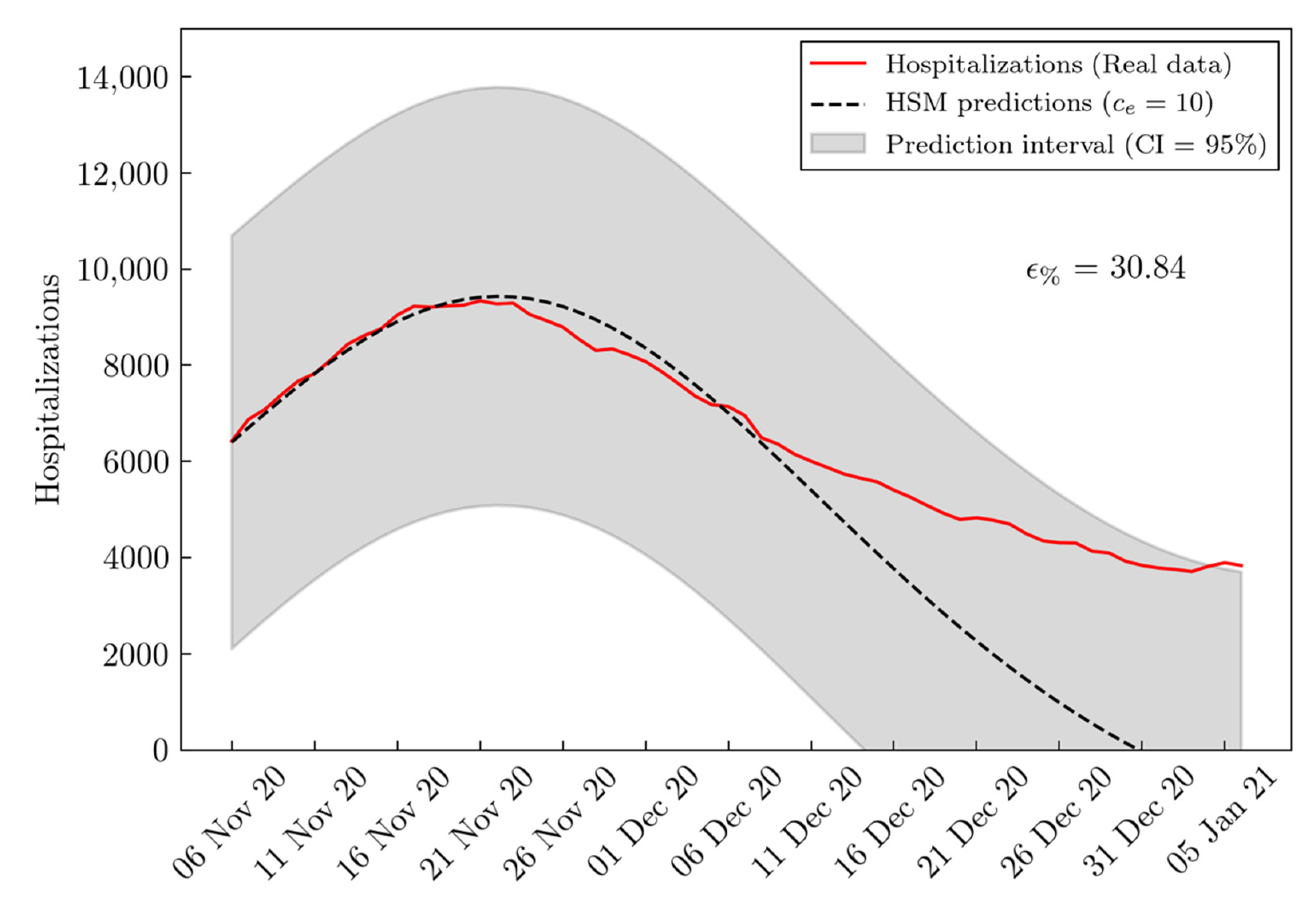
The daily reproduction number R d ( t ) has been estimated by using the next-generation matrix method [39] (see Appendix B):
R d ( t )   =   [   β   ρ   c ( t )   ( 1     q ) δ I ( t )   +   ϵ I   +   γ I   +   β     c ( t )   θ   ( 1     ρ )   ( 1     q ) γ A   ] S 0
Since R d ( t ) depends on the contact function c ( t ) , by modifying the variable L 1 in Equation (3), different daily reproduction number trends could be assessed in Lombardy during the first wave of the pandemic, with respect to the critical threshold R d ( t ) = 1 , (i.e., when the disease is endemic). When computed at the beginning of the pandemic ( t = 0 ), R d ( 0 ) represents the basic reproduction number (known as R 0 in literature), usually employed for evaluating the potential infectivity of a disease. Herd immunity (i.e., the minimum threshold allowing a population to become self-immune to a virus) has also been evaluated based on 9 March 2020 data in Lombardy, using the following equation proposed by Gorkin [40]:
i = 1   1   R 0
where i represents the portion of the population that needs to be immunized in order to reach the herd immunity threshold.

3. Results

Figure 3 reports the results of the simulations performed using BSM. For both panels, the x-axis reports the number of days from 9 March to 9 July 2020, whereas the y-axis reports the absolute number of hospitalizations. Real hospitalized people are depicted by a red line, whereas BSM predictions are shown in green through a dashed line. BSM hyper-parameters have been first initialized to the values reported in Appendix A (Table A2), and the corresponding predictions are shown in Figure 3a. BSM hyper-parameters have then been further tuned for the best setting, leading to a better fitting with respect to the actual hospitalizations trend observed (Figure 3b).
Moreover, the BSM best setting has been used as the starting point to perform a what-if analysis on the first pandemic wave, by taking advantage of the time-variant behavior of the contact function c ( t ) . The what-if analysis has been performed for assessing the effect of different lockdown durations on the hospitalizations trend (Figure 4a) and on the corresponding daily reproduction number R d ( t ) , leading to several scenarios (Figure 4b). The daily reproduction number was further evaluated on 9 March 2020 (t = 0) upon the adoption of containment measures for the first COVID-19 wave. The results reported in Figure 4b, show a value of R d ( 0 ) = R 0 = 2.625 . This value has been used for estimating the immunity threshold for Lombardy using Equation (11):
i = 1   1   2.625 = 0.619 = 61.9 %
Figure 5 shows the results obtained by means of the second order HSM hybrid model to predict hospitalization evolution during the second pandemic wave. As described in Section 2, the c e parameter in the c 3 ( t ) term of the contact function allows modelling the asymptotic presumed rate of personal contacts after the second wave lockdown imposed in Lombardy on 6 November 2020. Four different average rates of contact equal to 3, 6, 10, and 12 have been considered to assess the impact of different containment measures on the hospitalizations trend. Panel (a) reports the estimates of contacts evolution from 9 March 2020 to 31 December 2020, under four different scenarios based on the c e parameter. Panel (b) shows the results of the BSM prediction during the same observation period under the four different scenarios based on the c e parameter. An increasing loss of accuracy can be observed in the BSM with wider time windows, starting from 17 June 2020, producing an overestimate of hospitalizations in the period from the end of the first wave lockdown to the introduction of new containment measures during the second wave (15 October 2020). Panel (c) shows the results using HSM and four different rates of personal contacts during the lockdown period imposed in Lombardy on 6 November 2020: the lower the contact rate, and the earlier and lower the peak of the hospitalization curve. The comparison between BSM and HSM applications shows an improvement of more than 94% of HSM with respect to BSM (Table 1). The average percentage error ( ϵ % ) was also calculated for each contact scenario and, as it turned out, the c e = 10 scenario recorded the lowest error (2.39%) among all scenarios considered in the analysis (Figure 5c).
To emphasize such result, Figure 6 reports the hospitalizations trend as predicted by HSM compared with the actual number of hospitalizations in Lombardy, from 6 November to 8 December 2020. As shown, HSM predictions exhibited a very close match with actual hospitalizations data, falling into the confidence interval of prediction (CI: 95%) throughout the observed period.

4. Discussion

The present work suggests a hybrid approach based on Machine Learning that avoids recalculation of compartmental models’ hyper-parameters. This study shows that the proposed hybrid approach makes it possible to correct the expected loss of accuracy observed in the compartmental model when the considered time horizon increases.
Various mathematical models have been applied to obtain the most accurate predictions of COVID-19 hospitalizations in the first and second pandemic waves, according to social contact restrictions for lockdown, using the Lombardy region as a case study. As regards the first pandemic wave, from March to May 2020, a better setting of the classical BSM has been found through the fine-tuning of hyper-parameters, by means of a trial and error procedure that compares BSM predictions with real hospitalization data. This procedure allowed an improvement in hospitalizations predictions by about 26% (Figure 3b), with respect to forecasts achieved by the initial BSM version (Figure 3a). However, for the second wave, from October to December 2020, an HSM framework based on the classical BSM and a ML module, which relies on polynomial models that have been properly trained on real data, provided more accurate long-term predictions of COVID-19 hospitalizations than the traditional BSM. The application of both modelling approaches confirmed that containment measures, such as the lockdown and consequently contact reduction through social distancing, can heavily contribute to control the pandemic spread, depending on the magnitude of reduction of individual contacts and the length of the period: the lower the contact number and the longer the lockdown period, the lower the peak of hospitalizations and the farther the point the peak is reached (Figure 4a). The analysis of the different scenarios obtained through BSM may well support the selection of the most appropriate lockdown duration to reduce the number of hospitalized patients and relieve pressure or stress from the health system, while also limiting any negative impact on the economic and social systems. Results actually show that a 60-, 90- or 120-day lockdown would produce a very similar trend in terms of hospitalizations. The results achieved by the BSM best setting confirmed also the impact of lockdown duration on the daily reproduction number when it is above the critical threshold, meaning that the disease is spreading. Indeed, as reported in Figure 4b, a shorter lockdown causes R d ( t ) to persist above the critical threshold for more days, as compared with a longer lockdown. Furthermore, for each considered scenario, the results reported in Figure 4 show a dependence between the day in which R d ( t )   achieves the endemic critical threshold ( R d ( t ) = 1 ) and the day when the hospitalization peak is reached. The time interval between these two days might be related to the recovery period, estimated as 14 days according to Italian figures [34] and to the incubation period. Finally, the herd-immunity threshold of 61.9% is an optimistic result, since R 0 was computed on 9 March 2020 when some containment measures had already been introduced in Lombardy to reduce the COVID-19 spread. The adopted SEIR approach proved to properly model the trend of hospitalizations in Lombardy during the first pandemic wave. Unfortunately, due to the strong dependence of the BSM mathematical model on the initial conditions and on the hyper-parameters values that date back to 9 March 2020, an increasing loss of accuracy can be observed in the BSM with wider time window, as shown in Figure 5b, particularly, from the end of the first wave lockdown to the introduction of new containment measures during the second wave (15 October 2020). For this reason, the HSM framework has been applied. The appropriate variation of the c e parameter in the contact function that defines the asymptotic average value of contacts throughout the entire second wave, made it possible to outline four scenarios based on a different rate of personal contacts during the lockdown period imposed in Lombardy on 6 November 2020 [37]. Modelling the gradual decrease in the rate of personal contacts throughout the entire lockdown required using sigmoid functions in the contact function. Therefore, the results of applying the HSM framework depended on the contact function values during the transition period, that started on 15 October 2020, with the first Italian Prime Minister’s Decree [36]. The HSM framework proved very close to the hospitalization trend observed in Lombardy during the second wave of the pandemic (see Figure 5c), as it allowed to reduce the estimation error of more than 94% with respect to BSM in the hospitalization trend from 15 October to 5 November 2020, for all the considered scenarios. For the c e = 10 scenario, the hospitalizations trend predicted by HSM is very close to the real hospitalizations trend in Lombardy, from 6 November to 8 December 2020, with an average percentage error of 2.39%, as shown in Figure 6. Indeed, all the proposed scenario analyses depend on the choice of the contact function. The modelling procedures that have been proposed to describe the trend of personal contacts have proved appropriate for the estimation of different plausible scenarios about the trend of hospitalizations in Lombardy, both in the first and the second phase. In addition, the different scenarios related to the trend of contacts during the second wave suggest that the adoption of stricter containment measures with respect to the allowed rate of personal contacts might promote a more moderate trend of hospitalizations, with a lower peak and earlier in time. Under the most plausible scenario that sets the rate of allowed personal contacts to ten throughout the entire lockdown period in the second wave, predictions show a peak at around 9300 hospitalized patients, followed by a rapidly decreasing trend that should end on 1 January 2021. The main strength of the study lies in the development of a novel hybrid framework based on ML to reduce the errors that are usually introduced by mathematical compartmental models in the long term. The analysis was also stretched out to include the period from 8 December 2020 to 6 January 2021 by forecasting the contacts trend during the considered period. The results of the extended analysis are reported in Figure 7.
As clearly expected, HSM was not able to produce accurate forecasts in the period of interest ( ϵ % = 30.84%), even though forecasts fit in the 95% confidence interval. The reason for this depends on a number of factors related to the period of interest, including the quick alternation of different containment measures. As a matter of fact, the Prime Minister’s Decree of 3 November 2020 [37] imposed new restrictions on the country based on three risk scenarios related to increased critical levels (yellow, orange and red) in the various regions. The Decree provides for the assessment of restrictions based on the R t index value observed in each Italian region. The definition of the critical level per region will take place on a weekly basis and it will last 15 days. Each region shall then comply with the assigned critical level measures for at least two weeks. For this reason, the Italian situation is extremely dynamic and difficult to model. In addition, the vaccination campaign against COVID-19 was launched in Europe on 27 December 2020. Proper modelling should also account for the impact that vaccines are supposed to have on the epidemic curve. However, the developed framework is extremely general and although the focus of the present work was on the hospitalized people compartment, the framework could also have been efficiently used for other compartments of the SEIR mathematical model, thus enabling the accurate prediction of other COVID-19 variables as well. The modelling proposed for the contact function allows the assessment of different, more or less stringent containment measures based on a variable average number of contacts. Such measures help outline different hospitalization trend scenarios that are useful to monitor their impact on the national health system. For these reasons, the framework represents a valid and accurate decision support tool for policy-makers. Yet, as already said, the use of compartmental models strongly depends on the initial conditions and on a set of hyper-parameters that govern the evolution of the various compartments over time. The use of a model based on different time scenarios (i.e., phase two and any further phase of the pandemic) requires the definition of time variant hyper-parameters, for the model to adapt to changes in working conditions also in the long term. Clearly, in the case of complex compartmental models such as the BSM model with nine compartments used in the present study, redefining all hyper-parameters would mean having extremely fine-grained information and epidemiological point data available both in space and in time, along with using the appropriate estimation algorithms, as for instance those based on Maximum Likelihood. Consequently, the impossibility to redefine all hyper-parameters for very long-time frames causes a loss of accuracy in long-term predictions. To overcome this limitation, the authors exploited the Machine Learning. Moreover, as the contact function has a strong impact on the model predictions, the best definition of such function would require knowing the number of personal contacts at a regional level for the entire time frame under observation. The lack of such information led the authors to the assumption of a contact trend that is governed by the mobility trend provided by Apple. The choice of Lombardy as the case study for the proposed modelling approach can be a possible limit of the study. However, Lombardy has a larger population than various European countries, was highly affected by COVID-19 in both first and second wave and has large industrial and commercial activities determining a wide network of social contacts. However, the Italian regions have different public health systems and adopted nonidentical approaches for contrasting the COVID-19 pandemic, making a prediction model not suitable for any region, as somewhat different parameters should be included in the model. In conclusion, various mathematical forecasting models for the COVID-19 pandemic have been tried so far, but the choice of the best model depends on various assumptions and parameters which are valid in a specific context. Among them, the average number of daily contacts is of the utmost relevance to assess the effectiveness of confinement measures, due to the high transmission of SARS-CoV-2 through human contacts. However, the duration and strictness of containment measures have a substantial impact on the socio-economic fabric and the health system, therefore the estimate of different scenarios of the pandemic spread according to daily contacts and other parameters can be a valuable tool for choosing the most appropriate compromise solution to adopt.

Author Contributions

Conceptualization, A.G., G.A. (Giovanni Aloisio), G.A. (Gabriele Accarino) and V.A.; methodology, A.G., G.A. (Gabriele Accarino) and V.A.; software, A.G., G.A. (Gabriele Accarino) and V.A.; validation, G.A. and F.D.; formal analysis, A.G., G.A. (Giovanni Aloisio), G.A. (Gabriele Accarino), V.A. and F.I.; investigation, A.G., G.A. (Giovanni Aloisio), G.A. (Gabriele Accarino), V.A. and F.I.; resources, A.G., G.A. (Gabriele Accarino) and V.A.; data curation, A.G., G.A. (Gabriele Accarino) and V.A.; writing—original draft preparation, A.G., G.A. (Gabriele Accarino) and V.A.; writing—review and editing, G.A. and F.D.; visualization, A.G., G.A. (Gabriele Accarino) and V.A.; supervision, G.A. (Giovanni Aloisio); project administration, G.A. (Giovanni Aloisio); funding acquisition, Not Applicable. All authors have read and agreed to the published version of the manuscript.

Funding

This research received no external funding.

Institutional Review Board Statement

Not applicable.

Informed Consent Statement

Not applicable.

Data Availability Statement

Publicly available datasets were used in this study. As reported throughout the manuscript, these datasets can be found at the following links: https://github.com/pcm-dpc/COVID-19 (accessed on 21 July 2021); https://covid19.apple.com/mobility (accessed on 21 July 2021); http://dati.istat.it/?lang=en (accessed on 21 July 2021).

Acknowledgments

The authors would like to acknowledge Antonio Aloisio for his editing and proofreading work on this paper.

Conflicts of Interest

The authors declare no conflict of interest.

Appendix A

Compartmental Model Specification.
Table A1. Initial conditions for BSM on 9 March 2020.
DefinitionsValuesSources
S Susceptible10,025,948[17]
P Residents as of 31 October 201910,097,171[41]
D Deaths333[33]
H Hospitalized3242[33]
H + L + D Known Infected4823[33]
A + I Undetected Infected48,230[17]
A Undetected asymptomatic Infected32,153[17]
I Undetected symptomatic Infected16,077[17]
T Tests20,135[33]
Q Quarantined15,312[17]
E q Quarantined exposed24[17]
S q Quarantined susceptible15,288[17]
E Unknown exposed2212[17]
R Recovered646[33]
Table A2. Hyper-parameters used in the BSM differential equations.
DefinitionsValuesSources
L 1 Number of days of the first wave lockdown58BSM
T L 2 Number of days from the beginning of the first lockdown (9 March 2020) to the start of the second lockdown (6 November 2020)242BSM
Δ T L 2 Number of days for the gradual decrease in contacts after the second wave lockdown8BSM
c 0 Contact rate on 9 March 202010BSM
c b Lowest contact rate achieved during the first wave lockdown (9 March–18 May 2020)3[42]
c f Highest contact rate achieved after the first wave lockdown (9 March–18 May 2020)24BSM
c e Lowest contact rate after the second wave lockdown started on 6 November 2020{3, 6, 10, 12}BSM
r 1 Exponential decreasing rate of the contact function1.3768[16]
r f Exponential increasing rate of the contact function0.01BSM
α 1 Sigmoid function rate of decay0.8BSM
α 2 Sigmoid function rate of growth0.1BSM
β Probability of transmission per contact2.0011 × 10−8BSM
q Quarantined rate of exposed individuals1.887 × 10−7[17]
σ Transition rate of individuals exposed to the infected class1/14[43]
λ Rate at which the quarantined uninfected contacts were released into the wider community1/14[16]
ρ Probability of symptoms among infected individuals0.86834[16]
δ I 0 Initial transition rate of symptomatic infected individuals to the quarantined infected class0.3266[16]
1 / δ I F The shortest period of diagnosis0.3654[16]
r 2 Exponential decreasing rate of diagnose rate0.158BSM
δ q Transition rate of quarantined exposed individuals to the quarantined infected class0.1259[16]
γ I Recovery rate of symptomatic infected individuals0.33029[16]
γ A Recovery rate of asymptomatic infected individuals0.1BSM
γ H Recovery rate of hospitalized individuals0.0769BSM
α Disease induced death rate1.7826 × 10−7[16]
θ Infected rate of asymptomatic/symptomatic0.05[17]
ϵ I Rate of home isolation for infected individuals0.2[17]
ϵ q Rate of home isolation for quarantined exposed individuals0.2[17]
γ L Recovery rate for isolated infected individuals0.13978[17]
δ L Hospitalization rate for isolated infected individuals0.2[17]
BSM refers to the parameters that have been updated through the “trial and error” approach illustrated in the manuscript.
Formally, the Basic SEIR Model (BSM) used in our analysis is defined by the system of ordinary differential equations described by (1) in the manuscript and also used by Reno and colleagues [17]. The solution to the differential equation system is obtained by integrating differential equations over a time interval, starting from a set of initial conditions related to compartments, as reported in Table A1. The time evolution of each compartment is governed by a series of hyper-parameters whose values have been estimated based on the available data and information about the first pandemic wave. The full set of hyper-parameters is reported in Table A2. BSM is based on the SEIR model that was first introduced by Tang and colleagues [15,16] and then adapted to the Italian case by Reno and colleagues [17]. BSM has been designed by redefining some differential equations and the related hyper-parameters to achieve a better modelling of the hospitalizations trend in Lombardy. In particular, the following contact function proposed by Reno and colleagues [17],
c ( t ) = θ ( t T c   )   c 1   ( t ) + θ ( T c t )   c 2   ( t )
where:
c 1 ( t ) = ( c 0   c b ) e r 1 t + c b
c 2 ( t ) = ( c f   c b ) ( 1 e r 11 ( t T c ) ) + c b
θ ( t ) = {   1                                   i f   t < 0     0                         o t h e r w i s e
has been entirely reconstructed, as shown in Equations (2)–(7) in the manuscript. As discussed in the manuscript, the contact function c ( t ) has been designed as a linear composition of two terms c w 1 ( t ) and c w 2 ( t ) as shown by (2). Specifically, c w 1 ( t ) models the trend of personal contacts during the first pandemic wave and is expressed as a function of two time-varying terms c 1 ( t ) and c 2 ( t ) as reported in (3). The first term c 1 ( t ) , defined by (4), has been designed to model the exponentially decreasing number of contacts upon the adoption of containment measures for the first pandemic wave (9 March–18 May 2020). The second term c 2 ( t ) , has been used to model the increased number of contacts after gradually lifting containment measures at the end of the first wave lockdown. Moreover, c w 2 ( t ) models the trend of personal contacts during the second pandemic wave and is expressed as a function of the time-varying term c 3 ( t ) as reported in (6). The term c 3 ( t ) , defined by (7), has been added in the contact function to model the decreasing trend of contacts that was observed after the new containment measures put in place to control the pandemic spread during the second wave (16 October 2020 up to 6 January 2021). When formulating the contact function used by Reno and colleagues [17], both c 1 ( t ) and c 2 ( t ) terms can be left out through step function θ ( t ) , which allows an instant modelling of the trend of contacts during the transition phase and also upon entering and exiting lockdown. On the contrary, to achieve a more realistic modelling of the trend of contacts following the adoption of containment measures both in the first and in the second lockdown, the present analysis has selected appropriate sigmoid functions that enable the representation of smoothed transitions. It should also be noted that in our formulation, transitions entering and exiting lockdown are only managed by sigmoid functions, thus leaving info about the duration of the first and the second lockdown out of contact terms c 2 ( t ) and c 3 ( t ) , respectively. Finally, the c e parameter in the c 3 ( t ) term of the contact function allows modelling the asymptotic presumed number of personal contacts after the second wave lockdown imposed in Lombardy on 6 November 2020. Hence, c e allows estimating different hospitalization scenarios based on the pandemic evolution in Lombardy. The contact function is also parameterized by the c 0 ,   c b and c f   rates. In the original model by Tang and colleagues [16], c 0 has been defined as equal to 14.781 referring to Wuhan region in China. In our use case, this value should have been rescaled to c 0   = 13.469, according to (A5), to fit the Lombardy context with a population of about 10.097 million people [41],
W u h a n p o p :   14.781 = L o m b a r d y p o p : x
where Wuhan population has been estimated at about 11.081 million individuals [44]. However, the present analysis considered a lower value of c 0   = 10 to include the preliminary containment measures that had already been introduced in Lombardy on 9 March 2020. This value has also produced the best predictions with respect to the observed hospitalizations. The parameter   c b represents the lowest contact rate achieved during the lockdown period, that has been set to three according to the Italian Scientific Technical Committee report [42]. This document reports the average number of contacts per age group, considering a situation in which no containment measures are enforced on the population. As mentioned above, the lockdown was imposed on the entire Italian population from 9 March to 4 May 2020. It is safe to consider that the contact rate was only limited to home contacts in this period. Therefore, the value for c b has been obtained by calculating an average of the values for each age group. A broader discussion is needed for the c f parameter used to model the increasing trend of personal contacts between the two waves of the pandemic. Information about this parameter was not available at the time of writing, hence an intuitive approach has been applied using mobility data provided by Apple [35]. In Figure A1, the Apple mobility trends about “driving”, “walking” and “transit” are shown with respect to a baseline representing a reference mobility value registered on 13 January 2020 then before the adoption of any containment measures. After the end of the first wave lockdown (4 May 2020), an increasing trend can be observed with a peak higher than 100% (in the worst case) with respect to the baseline. Hence, the authors of the analysis assumed a similar trend for personal contacts, imposing a value above 100% with respect to the reference value c 0 that was previously estimated to model contacts before the first lockdown. Moreover, the recovery rates of hospitalized people ( γ H = 1 /   recovery   period H ) and asymptomatic infected individuals ( γ A = 1 /   recovery   period A ) have been redefined to adapt the model to the Italian case. The recovery period for hospitalized patients and asymptomatic infected individuals lasts 13 and 10 days, as reported in [34,45] respectively. Therefore, γ H = 0.0769 and γ A = 0.1 have been considered. Furthermore, δ I ( t ) (the diagnosis rate), which strongly depends on the resources available for detecting new cases, has been defined as in the work by Tang and colleagues, [16]:
  1   δ I ( t ) = (   1   δ I 0   1   δ I F )   e r 2 t +   1   δ I F
where, as reported in Table A2, δ I 0 is the diagnosis rate at the initial time ( t = 0 ) with δ I ( 0 ) = δ I 0 , δ I f is the fastest diagnose rate with l i m   t     δ I ( t ) = δ I f , and r 2 is the exponential decreasing rate.
Figure A1. Apple mobility trends and the corresponding presumed contacts. Mobility trends provided by Apple, expressed as percentage variation with respect to the baseline in Italy between 13 January and 9 November 2020, are reported by straight lines with values on the y-axis, left side. On the y-axis, right side, the presumed contacts have been reported according to the mobility trend.
Informatics 08 00057 g0a1

Appendix B

Evaluation of the Effective Reproduction Number
The effective reproduction number R e ( t ) is one of the most important epidemiological indices to control the behavior of an epidemic disease. It corresponds to the average number of new infections per infectious case in a population made up of both susceptible and unsusceptible hosts in a generic time instant t. If R e > 1 , the number of cases will increase, such as at the start of an epidemic [46].
The present study used BSM to estimate hospitalization in Lombardy from 9 March to 15 October 2020. R e ( t ) has been evaluated in each simulated day, leading to the definition of the effective daily reproduction number R d ( t ) . R d ( t ) has been evaluated by Tang and colleagues [15,16], using the next generation matrix algorithm [39], and its expression is reported in (A7).
R d ( t ) = [ c ( t ) β ( 1 q ) ( ρ δ I ( t ) θ ρ   α   θ ρ γ I θ + ρ γ A + δ I ( t ) θ + α   θ + γ I θ ) γ A ( δ I ( t ) + α + γ I ) ]
However, following the approach proposed by Reno et al. in [17], BSM adds a new compartment related to the isolated infected individuals (L) with respect to the SEIR model used by Tang and colleagues [15,16]. Thus, a new closed formula for R d ( t )   has been derived by applying the next generation matrix algorithm to BSM. Each step of the algorithm is presented as follows.
Let X be the vector of infected compartments, such as exposed (E), infected (I), asymptomatic (A), hospitalized (H), quarantined exposed (Eq), isolated infected (L). Let Y be the vector of uninfected compartments, such as susceptible (S), quarantined susceptible (Sq), and recovered (R). Let be the vector of new infection rates (transitions from Y to X) and V the vector of all other rates (not new infections).
X = [ E I A E q L H ] Y = [ S S q R ]         = [ β c ( t ) ( 1 q ) S ( I + θ A ) 0 0 β c ( t ) q S ( I + θ A ) 0 0 ]                 V = [     σ E σ ρ E + ( δ I ( t ) + ϵ I + γ I + α ) I σ ( ρ 1 ) E + γ A A ( δ q + ϵ q ) E q ϵ q E q ϵ I I + ( δ L + γ L + α ) L δ I ( t ) I δ q E q δ L L + ( γ H + α ) H     ]
Considering the following hypothesis regarding the Disease-Free Equilibrium (DFE), which is defined as the point at which no disease is present in the population, [47]:
  D F E = ( s * , 0 , , 0 )
it follows that
S = d S d t = [ ( β c ( t ) + c ( t ) q ( 1 β ) ) S ( I + θ A ) + λ S q ] | D F E = 0 ( β c ( t ) + c ( t ) q ( 1 β ) ) s * ( 0 ) + λ 0 = 0
Then, deriving vectors F and V with respect to X and evaluating them at the DFE point, we have:
F = d d X | D F E = [ 0 β c ( t ) ( 1 q ) β c ( t ) ( 1 q ) θ 0 0 0 0 0 0 0 0 0 0 0 0 0 0 0 0 β c ( t ) q β c ( t ) q θ 0 0 0 0 0 0 0 0 0 0 0 0 0 0 0 ]
V = d V d X | D F E =   [     σ 0 0 0 0 0 σ ρ δ I ( t ) + ϵ I + γ I + α 0 0 0 0 σ ( ρ 1 ) 0 γ A 0 0 0 0 0 0 δ q + ϵ q 0 0 0 ϵ I 0 ϵ q δ L + γ L + α 0 0 δ I ( t ) 0 δ q δ L γ H + α   ]
Computing the inverse of the matrix V and multiplying by F ,   the next-generation matrix F V 1 can be obtained as in the following:
F V 1 = [ β c ( 1 q ) ρ δ I ( t ) + γ I + ϵ I + β c ( 1 q ) ( 1 ρ ) θ γ A β c ( 1 q ) θ δ I ( t ) + γ I + ϵ I 0 0 0 0 0 0 0 0 0 0 0 0 0 0 0 0 β c q ρ δ I ( t ) + γ I + ϵ I + β c q ( 1 ρ ) θ γ A β c q δ I ( t ) + γ I + ϵ I β c q θ γ A 0 0 0 0 0 0 0 0 0 0 0 0 0 0 0 ]
Finally, by computing the dominant eigenvalue of the next generation matrix it is possible to obtain the following closed formulation for the daily reproduction number:
R d ( t ) = [ c ( t ) β ( 1 q ) ( ρ δ I ( t ) θ ρ ϵ I θ ρ γ I θ + ρ γ A + δ I ( t ) θ + ϵ I θ + γ I θ ) γ A ( δ I ( t ) + ϵ I + γ I ) ]
It should be noted that (A8), obtained for BSM, only differs from (A7) by Tang with regard to the rate of home isolation for infected individuals ( ϵ I ) which replaces the disease induced death rate ( α ) .

References

  1. Zhu, N.; Zhang, D.; Wang, W.; Li, X.; Yang, B.; Song, J.; Zhao, X.; Huang, B.; Shi, W.; Lu, R.; et al. A Novel Coronavirus from Patients with Pneumonia in China, 2019. N. Engl. J. Med. 2020, 382, 727–733. [Google Scholar] [CrossRef] [PubMed]
  2. WHO. Coronavirus Disease (COVID-2019) Situation Reports. 2020. Available online: https://www.who.int/emergencies/diseases/novel-coronavirus-2019/situation-reports (accessed on 21 July 2021).
  3. WHO. Naming the Coronavirus Disease (COVID-19) and the Virus That Causes It. 2020. Available online: https://www.who.int/emergencies/diseases/novel-coronavirus-2019/technical-guidance/naming-the-coronavirus-disease-(covid-2019)-and-the-virus-that-causes-it (accessed on 21 July 2021).
  4. Guan, W.-J.; Ni, Z.-Y.; Hu, Y.; Liang, W.-H.; Ou, C.-Q.; He, J.-X.; Liu, L.; Shan, H.; Lei, C.-L.; Hui, D.S.; et al. Clinical Characteristics of Coronavirus Disease 2019 in China. N. Engl. J. Med. 2020, 382, 1708–1720. [Google Scholar] [CrossRef]
  5. Romagnani, P.; Gnone, G.; Guzzi, F.; Negrini, S.; Guastalla, A.; Annunziato, F.; Romagnani, S.; De Palma, R. The COVID-19 infection: Lessons from the Italian experience. J. Public Health Policy 2020, 41, 238–244. [Google Scholar] [CrossRef] [PubMed]
  6. Prime Minister Decree. Further Implementing Provisions of the Decree-Law 23 February 2020, No. 6, with Urgent Measures in Relation to Containment and Management of the Epidemiological Emergency from COVID-19, Applicable Throughout the Country. (20A01605) G.U. General Series, no. 64 [in Italian]. 11 March 2020. Available online: https://www.trovanorme.salute.gov.it/norme/dettaglioAtto?id=73643 (accessed on 21 July 2021).
  7. Italian Institute of Health (ISS). Epicentro. Web Infographic—COVID-19 Integrated Surveillance Data in Italy. 2021. Available online: https://www.epicentro.iss.it/en/coronavirus/sars-cov-2-dashboard (accessed on 21 July 2021).
  8. Kermack, W.O.; McKendrick, A.G. Contributions to the mathematical theory of epidemics—I. Bull. Math. Biol. 1991, 53, 33–55. [Google Scholar] [CrossRef] [PubMed]
  9. Boquet, G.; Stigler, B. A Discrete Study of the SIR Model. 2004. Available online: http://citeseerx.ist.psu.edu/viewdoc/download?doi=10.1.1.601.265&rep=rep1&type=pdf (accessed on 21 July 2021).
  10. Chen, T.-M.; Rui, J.; Wang, Q.-P.; Zhao, Z.-Y.; Cui, J.-A.; Yin, L. A mathematical model for simulating the phase-based transmissibility of a novel coronavirus. Infect. Dis. Poverty 2020, 9, 1–8. [Google Scholar] [CrossRef] [Green Version]
  11. Integration of Ordinary Differential Equations. In Numerical Recipes: The Art of Scientific Computing; Cambridge University Press: Cambridge, UK, 2007; pp. 710–714.
  12. Prem, K.; Liu, Y.; Russell, T.W.; Kucharski, A.J.; Eggo, R.M.; Davies, N.; Jit, M.; Klepac, P.; Flasche, S.; Clifford, S.; et al. The effect of control strategies to reduce social mixing on outcomes of the COVID-19 epidemic in Wuhan, China: A modelling study. Lancet Public Health 2020, 5, e261–e270. [Google Scholar] [CrossRef] [Green Version]
  13. Kucharski, A.J.; Russell, T.W.; Diamond, C.; Liu, Y.; Edmunds, J.; Funk, S.; Eggo, R.M.; Sun, F.; Jit, M.; Munday, J.D.; et al. Early dynamics of transmission and control of COVID-19: A mathematical modelling study. Lancet Infect. Dis. 2020, 20, 553–558. [Google Scholar] [CrossRef] [Green Version]
  14. Yang, Z.; Zeng, Z.; Wang, K.; Wong, S.-S.; Liang, W.; Zanin, M.; Liu, P.; Cao, X.; Gao, Z.; Mai, Z.; et al. Modified SEIR and AI prediction of the epidemics trend of COVID-19 in China under public health interventions. J. Thorac. Dis. 2020, 12, 165–174. [Google Scholar] [CrossRef]
  15. Tang, B.; Wang, X.; Li, Q.; Bragazzi, N.L.; Tang, S.; Xiao, Y.; Wu, J. Estimation of the Transmission Risk of the 2019-nCoV and Its Implication for Public Health Interventions. J. Clin. Med. 2020, 9, 462. [Google Scholar] [CrossRef] [Green Version]
  16. Tang, B.; Bragazzi, N.; Li, Q.; Tang, S.; Xiao, Y.; Wu, J. An updated estimation of the risk of transmission of the novel coronavirus (2019-nCov). Infect. Dis. Model. 2020, 5, 248–255. [Google Scholar] [CrossRef]
  17. Reno, C.; Lenzi, J.; Navarra, A.; Barelli, E.; Gori, D.; Lanza, A.; Valentini, R.; Tang, B.; Fantini, M.P. Forecasting COVID-19-Associated Hospitalizations under Different Levels of Social Distancing in Lombardy and Emilia-Romagna, Northern Italy: Results from an Extended SEIR Compartmental Model. J. Clin. Med. 2020, 9, 1492. [Google Scholar] [CrossRef]
  18. Bollon, J.; Paganini, M.; Nava, C.R.; De Vita, N.; Vaschetto, R.; Ragazzoni, L.; Della Corte, F.; Barone-Adesi, F. Predicted Effects of Stopping COVID-19 Lockdown on Italian Hospital Demand. Disaster Med. Public Health Prep. 2020, 14, 638–642. [Google Scholar] [CrossRef] [PubMed]
  19. Rǎdulescu, A.; Williams, C.; Cavanagh, K. Management strategies in a SEIR-type model of COVID 19 community spread. Sci. Rep. 2020, 10, 1–16. [Google Scholar] [CrossRef]
  20. Giordano, G.; Blanchini, F.; Bruno, R.; Colaneri, P.; Di Filippo, A.; Di Matteo, A.; Colaneri, M. Modelling the COVID-19 epidemic and implementation of population-wide interventions in Italy. Nat. Med. 2020, 26, 855–860. [Google Scholar] [CrossRef] [PubMed]
  21. Ahmad, Z.; Arif, M.; Ali, F.; Khan, I.; Nisar, K.S. A report on COVID-19 epidemic in Pakistan using SEIR fractional model. Sci. Rep. 2020, 10, 1–14. [Google Scholar] [CrossRef]
  22. Kuzdeuov, A.; Baimukashev, D.; Karabay, A.; Ibragimov, B.; Mirzakhmetov, A.; Nurpeiissov, M.; Lewis, M.; Varol, H.A. A Network-Based Stochastic Epidemic Simulator: Controlling COVID-19 With Region-Specific Policies. IEEE J. Biomed. Health Inform. 2020, 24, 2743–2754. [Google Scholar] [CrossRef]
  23. Gaglione, D.; Braca, P.; Millefiori, L.M.; Soldi, G.; Forti, N.; Marano, S.; Willett, P.K.; Pattipati, K.R. Adaptive Bayesian Learning and Forecasting of Epidemic Evolution—Data Analysis of the COVID-19 Outbreak. IEEE Access 2020, 8, 175244–175264. [Google Scholar] [CrossRef]
  24. Bherwani, H.; Gupta, A.; Anjum, S.; Anshul, A.; Kumar, R. Exploring dependence of COVID-19 on environmental factors and spread prediction in India. Npj Clim. Atmos. Sci. 2020, 3, 1–13. [Google Scholar] [CrossRef]
  25. Battineni, G.; Chintalapudi, N.; Amenta, F. SARS-CoV-2 epidemic calculation in Italy by SEIR compartmental models. Appl. Comput. Inform. 2020. [Google Scholar] [CrossRef]
  26. Chintalapudi, N.; Battineni, G.; Amenta, F. Second wave of COVID-19 in Italy: Preliminary estimation of reproduction number and cumulative case projections. Results Phys. 2021, 28, 104604. [Google Scholar] [CrossRef]
  27. Zisad, S.; Hossain, M.; Hossain, M.; Andersson, K. An Integrated Neural Network and SEIR Model to Predict COVID-19. Algorithms 2021, 14, 94. [Google Scholar] [CrossRef]
  28. Alanazi, S.A.; Kamruzzaman, M.M.; Alruwaili, M.; Alshammari, N.; Alqahtani, S.A.; Karime, A. Measuring and Preventing COVID-19 Using the SIR Model and Machine Learning in Smart Health Care. J. Healthc. Eng. 2020, 2020, 8857346. [Google Scholar] [CrossRef] [PubMed]
  29. Tovissodé, C.F.; Lokonon, B.E.; Kakaï, R.G. On the use of growth models to understand epidemic outbreaks with application to COVID-19 data. PLoS ONE 2020, 15, e0240578. [Google Scholar] [CrossRef]
  30. Wu, Y.; Zhang, L.; Cao, W.; Liu, X.; Feng, X. The Generalized-Growth Modeling of COVID-19. Front. Phys. 2021, 8. [Google Scholar] [CrossRef]
  31. Worldometers. Coronavirus Update (Live): 76,104,704 Cases and 1,683,354 Deaths from COVID-19 Virus Pandemic. 2020. Available online: https://www.worldometers.info/coronavirus/ (accessed on 21 July 2021).
  32. Regione Lombardia. Dashboard COVID-19. 2020. Available online: https://www.regione.lombardia.it/wps/portal/istituzionale/HP/servizi-e-informazioni/cittadini/salute-e-prevenzione/coronavirus/dashboard-covid19 (accessed on 21 July 2021).
  33. Italian Civil Protection Department (ICPD). GitHub Data Repository. 2020. Available online: https://github.com/pcm-dpc/COVID-19 (accessed on 21 July 2021).
  34. Gemmi, F.; Bachini, L.; Forni, S. I Ricoveri per Covid-19 in Toscana. Prime Analisi. ARS Agenzia Regionale di Sanità Toscana. 2020. Available online: https://www.ars.toscana.it/collana-documenti-ars/2-articoli/4355-ricoveri-covid-19-in-toscana-prime-analisi-ars-toscana.html (accessed on 21 July 2021).
  35. Apple Mobility. COVID-19—Mobility Trends Reports—Apple. 2020. Available online: https://covid19.apple.com/mobility (accessed on 21 July 2021).
  36. Gazzettaufficiale.it. Prime Minister Decree, October 13th. 2020. Available online: https://www.gazzettaufficiale.it/eli/id/2020/10/13/20A05563/sg (accessed on 21 July 2021).
  37. Gazzettaufficiale.it. Prime Minister Decree, November 3rd. 2020. Available online: https://www.gazzettaufficiale.it/eli/id/2020/11/04/20A06109/sg (accessed on 21 July 2021).
  38. GOV.UK. COVID-19 Guidance for TIER 1 areas in UK. 2020. Available online: https://www.gov.uk/guidance/tier-1-medium-alert (accessed on 21 July 2021).
  39. van den Driessche, P.; Watmough, J. Reproduction numbers and sub-threshold endemic equilibria for compartmental models of disease transmission. Math. Biosci. 2002, 180, 29–48. [Google Scholar] [CrossRef]
  40. Gorkin, P. Numericon by Marianne Freiberger and Rachel Thomas. Math. Intell. 2015, 37, 96. [Google Scholar] [CrossRef]
  41. Dati.istat.it. Istat Statistics. 2020. Available online: http://dati.istat.it/?lang=en (accessed on 21 July 2021).
  42. CTS Report, Valutazione di Politiche di Riapertura Utilizzando Contatti Sociali e Rischio di Esposizione Professionale. April 2020. Available online: https://drive.google.com/file/d/1pe1gEp4-UAPxLW_vnqntAa4AT5D_nyR1/view (accessed on 21 July 2021).
  43. WHO. COVID-19 Virtual Press Conference Transcript. 7 September 2020. Available online: https://www.who.int/docs/default-source/coronaviruse/transcripts/covid-19-virtual-press-conference---7-september-corrects-name.pdf?sfvrsn=e00b8954_2#:~:text=The%2014%20days%20is%20based,the%20quarantine%20period%2014%20days (accessed on 21 July 2021).
  44. Treccani.it. Wuhan nell’Enciclopedia Treccani. 2020. Available online: https://www.treccani.it/enciclopedia/wuhan (accessed on 21 July 2021).
  45. Ministry of Health. Covid-19: Indicazioni per la Durata e il Termine Dell’isolamento e della Quarantena. Salute.gov.it. 2020. Available online: http://www.salute.gov.it/portale/nuovocoronavirus/dettaglioNotizieNuovoCoronavirus.jsp?lingua=italiano&id=5117 (accessed on 21 July 2021).
  46. Barratt, H.; Kirwan, M.; Shantikumar, S. Epidemic Theory (Effective & Basic Reproduction Numbers, Epidemic Thresholds) & Techniques for Analysis of Infectious Disease Data (Construction & Use of Epidemic Curves, Generation Numbers, Exceptional Reporting & Identification of Significant Clusters). Health Knowledge. 2020. Available online: https://www.healthknowledge.org.uk/public-health-textbook/research-methods/1a-epidemiology/epidemic-theory#:~:text=The%20effective%20reproductive%20number%20(R,the%20start%20of%20an%20epidemic (accessed on 21 July 2021).
  47. Morris, Q.A. Analysis of a Co-Epidemic Model. SIAM Undergrad. Res. Online 2011, 4, 121–133. [Google Scholar] [CrossRef]
Figure 1. The BSM architecture to forecast the hospitalizations trend in Lombardy (Italy). According to BSM, the population is divided into nine compartments: susceptible (S), exposed (E), infected (I), recovered (R), quarantined susceptible (Sq), asymptomatic (A), hospitalized (H), quarantined exposed (Eq), isolated infected (L). Interactions among compartments are depicted as directed segments, also reporting the related transition rates.
Informatics 08 00057 g001
Figure 2. Hybrid Susceptible, Exposed, Infected, and Recovered (SEIR) Model (HSM) framework Training and Inference phases.
Informatics 08 00057 g002
Figure 3. Basic SEIR Model (BSM) hospitalization predictions. BSM hospitalization predictions (dashed green line) compared with real hospitalization data (red line) in the period from 9 March to 9 July 2020. BSM hospitalization predictions, with the basic hyper-parameters setting reported in Table A2 of Appendix A, are shown in panel (a), whereas BSM hospitalization predictions, with the best setting of r 2   = 0.1 and γ A = 0.17529 hyper-parameters, are reported in panel (b).
Informatics 08 00057 g003
Figure 4. What-if Analysis based on different lockdown duration scenarios during the first wave and R d ( t ) estimation. (a) BSM best setting predicted hospitalizations based on different lockdown scenarios, with estimated hospitalization peaks (upward triangles) and days when the hospitalization reference threshold is reached (downward triangles), e.g., 10,000. (b) for each scenario, the corresponding daily reproduction number R d ( t ) is reported along with the estimated days (circles) in which the critical threshold is reached.
Informatics 08 00057 g004
Figure 5. COVID-19 hospitalization estimates in Lombardy according to different scenarios of personal contacts. HSM hospitalizations predictions assuming different scenarios of personal contacts during the second wave lockdown. The supposed contacts trend is shown in panel (a), whereas panel (b,c) show the different hospitalization scenarios using BSM and HSM, respectively. For each scenario, the average percentage error ( ϵ % ) from 6 November to 8 December 2020 is also reported.
Informatics 08 00057 g005
Figure 6. Real vs predicted hospitalizations in Lombardy. HSM predictions (dashed black line) for the average contact rate c e = 10 and real hospitalizations in Lombardy (straight red line) from 6 November to 8 December 2020 are reported. The 95% prediction confidence interval along with the average percentage error ( ϵ % ) between HSM hospitalization predictions and actual hospitalizations data are also reported.
Informatics 08 00057 g006
Figure 7. Real vs predicted hospitalizations in Lombardy. HSM predictions (dashed black line) for the average contact rate c e = 10 and real hospitalizations in Lombardy (straight red line) from 6 November 2020 to 6 January 2021 are reported. The 95% prediction confidence interval along with the average percentage error ( ϵ % ) between HSM hospitalization predictions and actual hospitalizations data are also reported.
Informatics 08 00057 g007
Table 1. Comparison between BSM and HSM in the period 15 October–5 November 2020, using RMSE 1.
c e BSM RMSEHSM RMSEImprovement (%)
32834.34151.6394.65
62864.07128.0395.53
102905.20103.9696.42
122926.4395.7896.73
1 RMSE = Root Mean Squared Error.
Publisher’s Note: MDPI stays neutral with regard to jurisdictional claims in published maps and institutional affiliations.

