Where Is My Mind (Looking at)? A Study of the EEG–Visual Attention Relationship

Abstract

Visual attention estimation is an active field of research at the crossroads of different disciplines: computer vision, deep learning, and medicine. One of the most common approaches to estimate a saliency map representing attention is based on the observed images. In this paper, we show that visual attention can be retrieved from EEG acquisition. The results are comparable to traditional predictions from observed images, which is of great interest. Image-based saliency estimation being participant independent, the estimation from EEG could take into account the subject specificity. For this purpose, a set of signals has been recorded, and different models have been developed to study the relationship between visual attention and brain activity. The results are encouraging and comparable with other approaches estimating attention with other modalities. Being able to predict a visual saliency map from EEG could help in research studying the relationship between brain activity and visual attention. It could also help in various applications: vigilance assessment during driving, neuromarketing, and also in the help for the diagnosis and treatment of visual attention-related diseases. For the sake of reproducibility, the codes and dataset considered in this paper have been made publicly available to promote research in the field.

1. Introduction

Saliency heatmap estimation is a field of research at the cutting edge of technology today. Visual saliency maps represent the probability of an area in a visual scene to attract the participant’s visual attention; concretely, a visual saliency map is a single-channel image with each pixel representing the probability between 0 and 1 to be observed [1]. Estimating with precision the region of the field of view where humans focus is a great help for many computer vision applications. In most of the works aiming to estimate images that represent the region of interest in the field of view, also called the visual saliency map, the considered modalities are often images and videos [2,3].

Nowadays, machine learning (ML) and the topics deriving from it have seen a huge increase in interest. More and more publications and research projects related to novel deep learning (DL) algorithms have been presented in recent years. Although ML algorithms tend to be used for more image-related fields, a growing interest has been noticed in the medical domain [4]. It was observed that the use of ML algorithms may be an interesting opportunity to improve diagnosis, help the works of specialists, and have a better understanding of biomedical signals.

As of today, the existing works aiming to estimate visual saliency are based on images [1,2,3,5], the estimation is based on the considered image and does not take into account the participant specificity, each image presenting a visual salience map independently of the participant viewing the image. Thus, it could be interesting to exploit the scientific research proving the relationship between brain activity and attention mechanism [6] by estimating visual saliency from biomedical signals. The goal of this work is not to beat the results provided by image-based methods but to investigate this novel relationship.

On another hand, the increasing amount of data and their democratization have led to an increase in research projects in Brain–Computer Interfaces (BCI). BCI are applications aiming to create a link between human brains and computer interfaces through biomedical signals. This connection can be (non-)invasive and more or less expensive depending on the considered biomedical signals. Among the different types of biomedical signals considered in existing research projects, electroencephalogram (EEG) representing electrical brain activity seems to be prone for this type of application. The motivations are based on their ease of use and relatively low cost compared to other techniques while maintaining a high fidelity for signals acquisition. Moreover, it has been proven that specific EEG patterns are observed during visual attention-related tasks [7].

Another type of signal directly related to visual attention is eye-tracking signals measuring the region of a visual scene toward which the gaze is directed. In this context, it has been considered to investigate the relationship between eye tracking and EEG through BCI. For this purpose, we propose a novel framework aiming to estimate visual saliency maps from electrophysiological recordings.

The contribution of this paper can be summarized in three points: (1) an adaptation for raw signals of the existing methods for EEG’s features representation under images form; (2) a novel feature extraction method representing EEG signals in lower subspace; (3) a framework estimating the visual saliency map from electrophysiological signals.

2. Related Work

The related work has been split into three subsections: (1) deep learning approaches for EEG processing, presenting different methods based on DL to process EEG; (2) EEG-based attention estimation, introducing the research projects related to attention in the context of EEG; (3) visual saliency estimation, showing the existent works aiming to estimate the saliency map from several modalities.

2.1. Deep Learning Approaches for EEG Processing

As previously mentioned, ML algorithms have attracted interest for some time now. It has also been the case in the context of biomedical signal processing and brain imaging research. More specifically, in the case of electroencephalogram signals processing, several deep learning approaches have been considered for different purposes [8]. In most of the cases, EEGs are considered as an array $X\in {\mathbb{R}}^{t\times elec}$ with t representing the time evolution and $elec$ representing the number of considered electrodes. A non-exhaustive list of works considering DL algorithms with EEG is the following:

• The use of convolutional neural networks (CNN) has been considered to extract feature from EEG signals. One of the best known models is EEGNet presented by Lawhern et al. [9]. This network aims to estimate motor movements and detect evoked potentials (specific pattern in electrophysiological signals seen after stimuli apparition) through a sequence of convolution filters with learnable kernels. These kernels extract the spatial and/or temporal features from the signal according to the considered shape (x-axis representing the time evolution and y-axis representing the considered channels).
• One of the other methods considered to process EEG is the use of graph networks. With this approach, the EEG is considered as a graph (with vertices corresponding to electrodes and edges being proportional to their distance) evolving over time. The method based on Regularized Graph Neural Networks proposed by Zhong et al. [10] presents the best results for emotion estimation from EEG.
• Another approach that has already been considered for a wide range of application in EEG processing is based on recurrent neural networks (RNN). These kinds of networks have already proven their ability to extract the spatial [11] and temporal [12] information from brain activity signals. In the work of Bashivan et al. [12], Bashivan et al. consider a model composed of a different layer of CNN and RNN to estimate motor movements from EEG.
• Over the last years, an emerging method has been considered: the use of a generative adversarial network (GAN) for EEG processing. GAN is a family of neural networks where two networks (i.e., generator and discriminator) are trained in an adversarial manner: the discriminator aims at detecting if a given modality has been artificially generated or corresponds to the ground truth, and the generator tries to fool the discriminator by generating modalities very close to reality [13]. GANs have already been used for generating images representing thoughts and/or dreams [14,15]. Although this research field is still under development, the authors have high hopes that one day, it will be possible to visualize our thoughts or dreams.

In addition to the different DL models used for estimation and regression from brain activity, it is also possible to consider different feature extraction and representation methods. In [9], they directly considered the raw signal and let the models extract the most significant feature. On the other hand, in [11,12], they considered well-known feature extraction methods expressing the spectral [12] and temporal information [10,11] from signals. Moreover, in [12], they consider a more visual representation of EEG features under a more understandable form. In their approach, they consider the position of each electrode in the 3D frame and create an image within which the location of pixels and electrodes are correlated, and their value is related to the feature value in the specific location.

2.2. EEG-Based Attention Estimation

Liang et al. [16] present an approach to estimate visual saliency features from EEG. The considered methodology consists of a joint recording of EEG while watching video clips. Saliency features representing the degree of attention and average position of the center of interest in the video. The presented results were encouraging for further study and indicate the existence of a relationship between visual attention and brain activity. On the other hand, different datasets aiming to estimate the attention state from biomedical signals have been published. Cao et al. [17] and Zheng et al. [18] considered recordings of EEG and eye-tracking signals to estimate the attention state of a participant during specific tasks. Zheng et al. [18] show that it is possible to estimate the attention state from these joint recordings in many cases.

The lack of in-depth studies aiming to investigate the relationship between EEG signals and visual saliency has been a motivation for the creation of a framework aiming to investigate the relationship between these two modalities.

2.3. Visual Saliency Estimation

Visual saliency estimation is a field at the cutting edge in the computer vision domain. There exist a lot of different models aiming to estimate visual saliency from different modalities. In most of the cases, the goal of these models is to estimate the visual saliency region from images as reported in the MIT/Tuebingen Saliency Benchmark [19], including all the existing models. Among the existing works, a certain amount of the proposed methods was based on the succession of encoding (composed of successions of convolution and max-pooling layers) and decoding (resp. succession of convolution layer and upsampling layers) networks as in the works of Kroner et al. [20] and Pan et al. [3] being in the best results among the state-of-the-art works.

3. Proposed Method

The goal of our work is to combine the existing DL methods to study the relationship between electrophysiological signals and a visual saliency map. The framework is divided into three models:

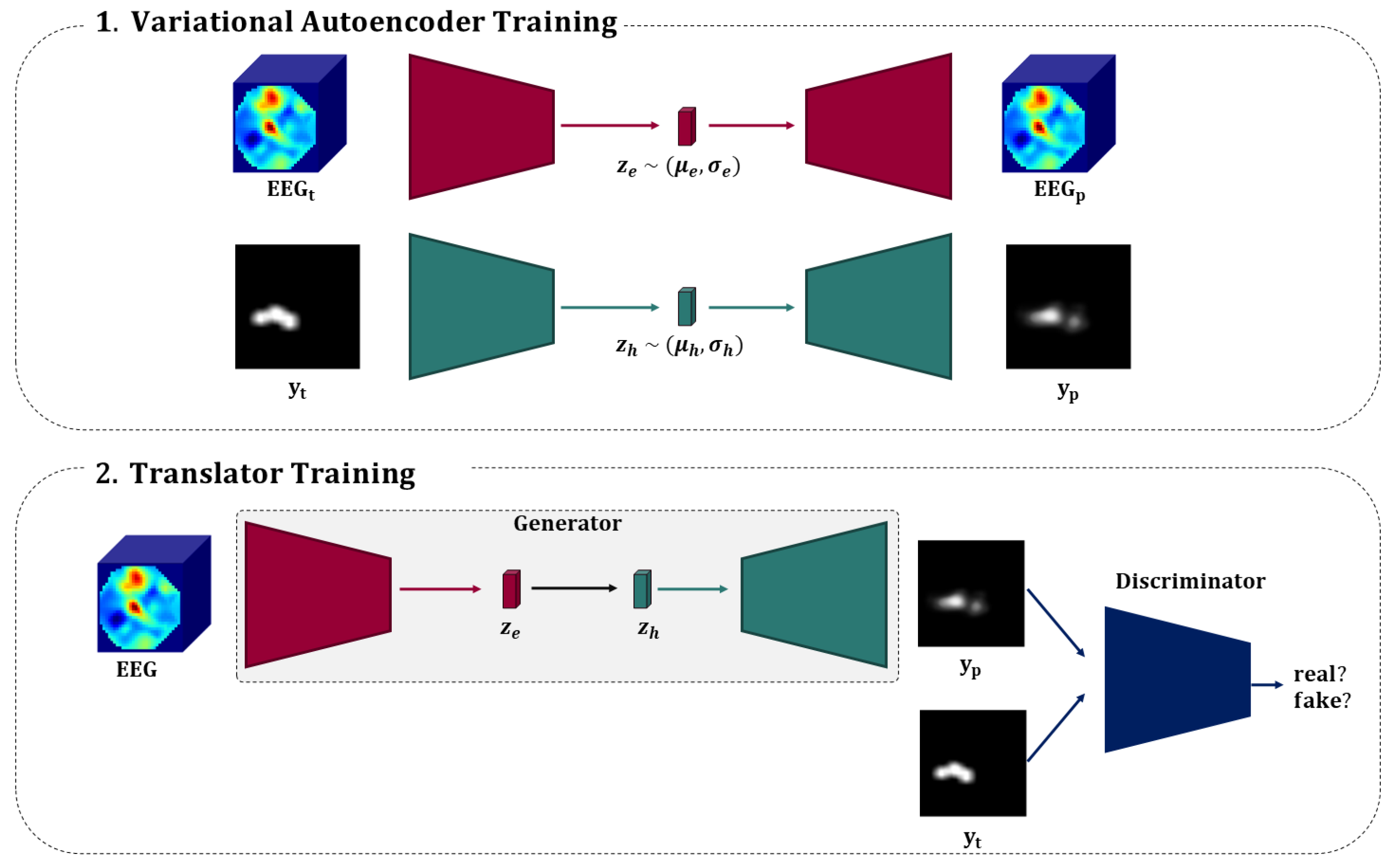
• A variational autoencoder (VAE) aiming to represent the saliency images in a shorter subspace called latent space. This VAE will have two roles: recreating the saliency images that represent the participant visual attention; and representing the images in a completed and continuous latent space [21].
• A VAE aiming to represent the EEG in the latent space. As for the previous model, the aim of EEG VAE is also to minimize the error between the EEG and its reconstruction and to create a continuous and completed representation of the signals in the corresponding latent space.
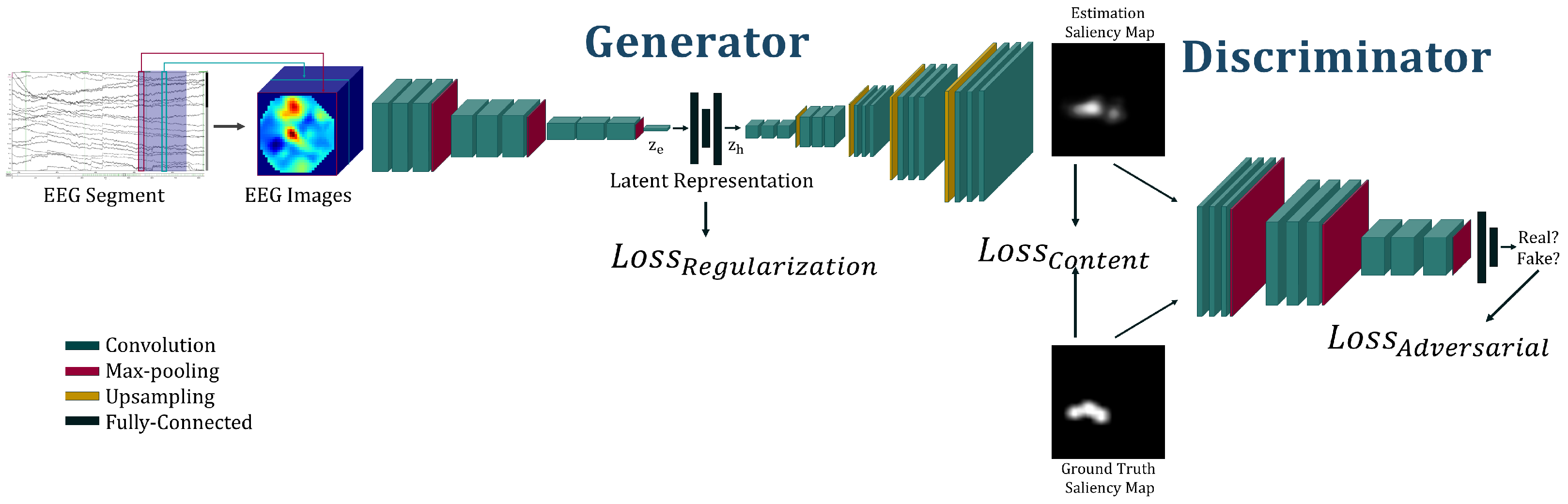
• A GAN binding the EEG and map latent space with the help of the two VAEs already described. In addition, a discriminator is also used to classify the images from synthetic (i.e., created by our model) vs. real (i.e., real saliency maps created from eye-tracking recording).

Figure 1 shows the framework pipeline separated in two steps: the training of both VAEs and the training of the saliency generator part. The choice of considering VAE instead of the conventional deep autoencoder is motivated by the fact that there is no one-to-one relationship between brain activity and visual attention (by one-to-one relationship, Stephani et al. [22] mean that one and only one brain activity corresponds to one and only one map representing attention). This phenomenon, showing that different brain activation may correspond to a single task (and vice versa), has been studied by Stephani et al. [22]. Moreover, this aspect is enhanced by the fact that it is difficult to extract information from electrophysiological signals due to their trend to be prone to noise and artefacts. The use of VAE instead of conventional AE enables to estimate the distribution (characterized by mean and standard deviation) of the latent space and to study the relationship between their distribution instead of creating a one-to-one relationship between latent vectors.

We separated the proposed methods into four subsections, each of them being a specific step of our work: (1) Autoencoding Saliency Map; (2) Autoencoding EEG Signals; (3) Translation Network mapping the latent spaces distributions; (4) Training Methodology.

3.1. Autoencoding Saliency Map

From raw eye-tracker recordings, it is possible to create a visual saliency map representing the area of attention in an image of one channel with values between 0 and 1 representing the degree of visual attention on specific pixels and their neighbors. It can also be considered as a probability for a given pixel to be watched or not.

During the experimentation, the eye-tracker has been jointly recorded with EEG. First, the recordings have been separated into trials corresponding to a specific time. Then, the discrete eye-tracking measurements have been projected onto 2D images (one per trial). After that, the eye-tracker accuracy has been taken into account by considering circles of radius proportional to the error rate despite discrete points. Finally, Gaussian filtering has been applied to the images with a kernel size ratio corresponding to the eye-tracker field of view. The images’ generation has been inspired by Salvucci et al. [23].

Given the visual saliency images, a VAE has been trained to represent them in a lower subspace. The considered network architecture is based on the ResNet proposed by He et al. [24]. We consider for the encoding part four stacks of ResNet layer, each composed of three convolutional layers and batch normalization, each stack except the last being separated by a max-pooling operation. A similar approach has been considered for the decoding part with an upsampling layer instead of a max-pooling operation; the padding has been adapted to ensure that the output size matches the input.

The goal of this network is double: (1) recreating an image as faithfully as possible to the original saliency map via a representation in shorter latent space; (2) creating a continuous and complete latent-space and therefore not favoring one dimension among others.

After some experimental tests, it has been constated that the VAE tend to slightly overfit after a certain amount of epochs. To reduce this issue and to build a more robust network, a data augmentation policy has been considered. To keep the physical behavior behind a visual saliency map, the data augmentation process had to be well designed. For this reason, we have considered for each training sample of each batch from the training set a random horizontal flip with a probability of 0.5 (the stimuli being equally disposed at the right and left part of the screen, as shown in Section 4.1) and a random vertical and horizontal translation between −5 and +5 pixels. This method helped to generate a wider range of visual saliency map with a lower error rate between the initial image and its reconstruction with a better representation of the latent space.

3.2. Autoencoding EEG Signals

EEG can be considered as a two-dimension time series, the first corresponding to time evolution and the second corresponding to the considered electrodes. Unlike Bashivan’s approach [12], consisting of creating EEG images from spectral feature maps based on the electrodes’ spatial location, the process to construct our EEG images is the following:

• Separating the total recording in trials leading to an array of dimension $[n_{trials}\times t\times n_{electrodes}]$.
• For each trial, downsampling the signals after low-pass filtering to extract the general signal evolution and to ignore the artefacts contribution. Preprocessing is at the same time applied to remove the noise and remaining artefacts.
• From the regular electrode position on the scalp, an azimuthal projection is applied to represent their location in a 2D frame.
• The samples composing the trials are taken separately. These samples are projected in a 2D coordinate frame as mentioned at the previous step, and a bicubic interpolation is applied to consider a continuous representation of information. The process is repeated for all the samples, and each projection is concatenated to lead to an image with a number of channels corresponding to the number of temporal samples after the signal downsampling.
• The statistical distribution of the images set has also been normalized around a mean of 0 and a standard deviation of 1.

This maps representation of EEG allows keeping the spatial (in the first and second dimension) and temporal (between channels) relationship between samples. For clarirty, the maps generated from EEG are mentionned as EEG images in the paper. Moreover, this methodology better suits for CNN than the array representation of EEG. It enables the consideration of squared shape kernels unlike the older models considering unidimensional kernels for feature extraction from EEG [9].

In a similar way to the image VAE, the EEG images have been passed through a VAE to reduce the EEG dimension and to represent them in a continuous and completed subspace. For this purpose, the VAE has been trained with the images-based EEG.

A similar methodology to that for the saliency map has been considered to construct the most robust network as possible. To that end, a random signal following a Gaussian distribution of zero mean and standard deviation = 0.25 has been added to EEG images to increase the model stability and to have a better understanding of the difference between noise and EEG. In addition, some pixels composing the EEG images have been supposed to remain equal to zero; these groups of pixels correspond to the region of the space where there are no electrodes. A checking was set up to verify that those regions of the images remained equal to zero.

3.3. Generator Network Mapping the Latent-Space Distributions

From the representation of the saliency map and EEG in their corresponding shorter subspace, the possibility of mapping the two distributions has been investigated. For this purpose, several approaches have been tested; however, for the paper clarity, only the ones presenting the best results have been presented.

As mentioned above, previous works have already investigated the GAN architecture for EEG processing [14,15]. However, these last few consider a different EEG signal representation, based on arrays; thus, a novel architecture suiting with our EEG images representation has been designed.

One of the most important barriers in this paper was to create a model permitting the estimation of a saliency map from EEG without considering a one-to-one correspondence between modalities. To solve this issue, a GAN approach has been considered with a generator aiming to recreate the image latent representation from EEG latent representation combined with a discriminator aiming to distinguish the images generated by the generator (composed of the combination of the encoding and decoding part of the VAEs presented in the previous subsection). In addition, as it is the case in several approaches [13], noise following a normal centred distribution (i.e., mean = 0 and std = 1) has been concatenated to the latent vector at the center of the generator. This concatenation aims to guide the generator for the saliency map generation.

The overall architecture of the networks aiming to translate the EEG space into image space is represented in Figure 2. As seen in this figure, the generator consists of the concatenation of the encoding part of EEG VAE and decoding part of Saliency VAE through a generator composed of fully-connected (FC) layers. Moreover, as mentioned above, a discriminator has also been placed at the end of the model.

3.4. Training Methodology

As already mentioned, the generator model consists of the concatenation of two parts of pre-trained models. The training policy can be considered in several key steps:

First, there is the separate training of the two VAE. During this training, the goal is to reduce a combination of a content loss, aiming to reduce the reconstruction error, and a regularization loss, promoting a continuous and completed distribution in the latent subspaces. The considered content loss for image VAE is the binary cross-entropy, the values of the images being included between 0 and 1. For the EEG VAE, an MSE loss has been considered for the opposite reason (EEG images taking values <0 and >1). The minimization policy for the two models can be formulated as for the heatmap:

$$\begin{array}{c}\hfill {\mathcal{L}}_h\left({\theta }_h\right)={\mathcal{L}}_{cont}+{\mathcal{L}}_{reg}\\ \hfill =BCE(y_t,y_p)+0.5\ast KLD({\mu }_i,log\left({\sigma }_i\right))\end{array}$$

(1)

with ${\theta }_h$ representing the model parameters of the image VAE, $y_t$ representing the ground truth saliency map, $y_p$ representing the reconstructed map, and ${\mu }_i$ and ${\sigma }_i$ representing the mean and variance of the estimated latent space. For the losses, BCE represents the binary cross entropy loss and KLD represents the Kullback–Leibler divergence [21]. For the EEG:

$$\begin{array}{c}\hfill {\mathcal{L}}_e\left({\theta }_e\right)={\mathcal{L}}_{cont}+{\mathcal{L}}_{reg}\\ \hfill =MSE(EE{G}_t,EE{G}_p)+0.5\ast KLD({\mu }_i,log\left({\sigma }_i\right))\end{array}$$

(2)

with ${\theta }_h$ representing the model parameters of the EEG VAE, $EE{G}_t$ representing the ground truth EEG, $EE{G}_p$ representing the reconstructed EEG, and ${\mu }_i$ and ${\sigma }_i$ representing the mean and variance of the estimated latent-space. During the training of both VAE, a phase of sampling is necessary to estimate the current latent projection from its mean and standard deviation. For this purpose, we use the reparameterization trick [21], this last considering a random variable following a Gaussian distribution with mean = 0 and standard deviation = 1 to solve the backpropagation issue that the direct sampling causes.

Then, the generator model has been created by concatenating the two parts of the VAE and linking them with FC layers. Moreover, the discriminator has also been added after the decoding part. After the architecture creation, all the weights composing the decoder and encoder parts have been fixed (i.e., no gradient descent has been applied on those parameters). An exception has been made for the last layers of the encoder and the first layers of the decoder (i.e., model parts directly connected to the latent space) to promote the networks’ fine-tuning.

During the training of the generator, three losses have been considered: a content loss to assess the similarity between the ground truth and the created maps; an adversarial loss aiming to distinguish the generated vs. the ground truth; and a regularization loss assessing that the latent-space representation remains continuous and complete. The competition between the generator and the discriminator helps for the generation of maps being difficult to differentiate with the ground truth. The considered metrics for each of these losses were: the BCE for the content loss and the adversarial loss and KLD for the regularization loss. The minimization paradigm to train the generator can be formulated as:

$$\begin{array}{c}\hfill \mathcal{L}\left(\theta \right)={\mathcal{L}}_{cont}+{\mathcal{L}}_{reg}+{\mathcal{L}}_{adv}\\ \hfill =BCE(y_t,y_p)+0.5\ast KLD({\mu }_i,log\left({\sigma }_i\right))+\\ \hfill BCE(D\left(y_t\right),1)+BCE(D\left(y_p\right),1)\end{array}$$

(3)

with ${\theta }_h$ representing the model parameters, $y_t$ representing the ground truth saliency map, $y_p$ representing the reconstructed map, ${\mu }_i$ and ${\sigma }_i$ representing the mean and variance of the estimated latent spaces, and $D{(}_{})$ being the output of the discriminator.

4. Experiments

In this section, we first present the considered methodology for the joint acquisition of EEG and eye-tracking signals. Then, the implementation details of the models will be described, and finally, the proposed metrics for our approach evaluation will be presented in the last subsection.

4.1. Dataset Acquisition

The signals considered in this paper have been acquired on 32 healthy participants (14 women and 18 men) recruited among the University of Mons community during a 15 min long session; each participant took part in only one session. The signal acquisition protocol consists of a short video game in virtual reality (VR) where the participant is asked to direct his gaze on stimuli corresponding to an object appearing in a random position of the field of view; a more complete description of the sustained and selective attention tasks is given in [25]. The study and experimental protocol were approved by the Ethical Board of the Faculty of Psychology and Education of the University of Mons.

During the proceeding of the tasks, the eye position and EEG have been synchronously registered. EEG has been recorded with a 32-electrode biomedical headset (actiCHamp from BrainVision) following the 10/20 electrodes disposition [26]. To allow recording EEG while participants were wearing the VR headset, the original 10/20 electrodes disposition has been adapted P3 → AF3; Pz → FCz; P4 → AF4.

On the other hand, the eye-tracker has been registered with the dedicated device placed into the VR headset (HTC Vive Pro Eye with an integrated eye-tracker). After the registration, trials have been extracted from the total recording by segmenting both signals around the stimuli apparition: we consider for both physiological signals the beginning of the segment one second before and the end three seconds after the stimuli appearance. EEG signals were recorded with the dedicated constructor software and other signals with the VR game [25] designed with Unity Game Engine [27]; the synchronization has been performed with keyboard input simulation, the latter being used in BrainVision Recorder to annotated EEG signals.

This dataset has been recorded in the context of a research project aiming to investigate the relationship between attention and brain activity. For this purpose, a pipeline aiming to record physiological signals in VR has been designed. To promote results reproducibility and research in this domain, the signals acquired have been made publicly available.

4.2. Implementation Details

Given the raw EEG considered as an array of dimension $[n_{trials}\times n_{channels}\times n_{samples}]$ with $n_{trials}=4000$ being the total number of trials for all the sessions, $n_{channels}=32$ being the total number of electrodes of the EEG cap, and $n_{sample}=t_{length}\times f_{sampling}=4\ast 500=2000$ being the total number of samples composing the EEG signal. The signals have been downsampled with a ratio $=5$ and passed through a low-pass filter with a cut-off frequency $=35$ Hz. Then, EEG images have been created from the preprocessed signals with the methodology explained in Section 3.2, the result dimension being $[n_{trials}\times n_{down}\times h\times w]$ with $n_{down}=401$ being the amount of samples after downsampling and $h=32$ and $w=32$ being the height and width of the corresponding created image.

Moreover, the saliency map built from the eye-tracking recording can be considered as an image of one channel with a height $=45$ and width $=81$, the ratio between the width and height being deduced from the VR headset resolution should be equal to $1.8$. One visual saliency map has been created for each trial with a corresponding EEG image. Moreover, the CNN being used to consider squared image, empty borders has been added at the top and the bottom of the visual saliency map.

As explained earlier, the final framework is divided into two models: the generator and the discriminator. As in many other projects considering GAN, the training policy consists of competition between these two models. The aim of the discriminator is to distinguish the generated visual map among the ground truth and simultaneously to bias the discriminator by generating a saliency map as close as possible to reality. The proposed architecture of the generator and discriminator is described in

Table 1. Architecture of the generator network.

	Generator
Network Part	Layer	Int/Out Channels
EEG Encoder	Conv2D-3	401/256
	Conv2D-3	256/256
	Conv2D-3	256/256
	Conv2D-3	256/256
	Maxpool-2	256/256
	Conv2D-3	256/512
	Conv2D-3	512/512
	Conv2D-3	512/512
	Maxpool-2	512/512
	Conv2D-3	512/512
	Conv2D-3	512/512
	Flattening Layer
	Linear	512/256
	Linear	256/64
Distrib. FC	Linear	64/64
	Sampling Layer
	Noise Cat	64/128
	Linear	128/256
	Linear	256/64
Saliency Decoder	Linear	64/512
	UnFlattening Layer
	Upsampling-2	512/512
	Conv2D-3	512/512
	Conv2D-3	512/512
	Conv2D-3	512/512
	Upsampling-3	512/512
	Conv2D-3	512/256
	Conv2D-3	256/256
	Conv2D-3	256/256
	Upsampling-3	256/256
	Conv2D-3	256/128
	Conv2D-3	128/128
	Conv2D-3	128/128
	Upsampling-3	128/128
	Conv2D-3	128/64
	Conv2D-3	64/64
	Conv2D-3	64/64
	Upsampling-2	64/64
	Conv2D-3	64/4
	Conv2D-3	4/4
	Conv2D-3	4/1

and

Table 2. Architecture of the discriminator network.

Discriminator
Layer	Int/Out Channels
Conv2D-3	1/3
Conv2D-3	3/32
Conv2D-3	32/32
Conv2D-3	32/32
Maxpool-2	32/32
Conv2D-3	32/64
Conv2D-3	64/64
Conv2D-3	64/64
Maxpool-2	64/64
Conv2D-3	64/128
Conv2D-3	128/128
Conv2D-3	128/128
Maxpool-2	128/128
Conv2D-3	128/256
Conv2D-3	256/256
Conv2D-3	256/256
Flattening Layer
Linear	256/64
Linear	64/1

.

Adam optimizers have been used to train the three models. A learning rate $={10}^{-5}$ with momentum $=0$ has been considered to train both VAEs. For the GAN approach, we consider two optimizers, one for each part, a learning rate $={10}^{-7}$ with a momentum $={10}^{-5}$ for the generator and a learning rate $={10}^{-5}$ with a momentum $={10}^{-8}$ for the discriminator. The choice of a very low learning rate for the generator part has been motivated by the fact that the major part of the network was already trained and that we tried to not modify the model’s ability to extract features from each modality (i.e., visual saliency heatmap and EEG images). The saliency VAE has been trained on 2000 epochs and the EEG VAE has been trained on 3000 epochs. The merged model has been trained on 1500 epochs; however, the training was manually stopped if the convergence point was achieved. All the weights, codes, and signals are freely available on https://bit.ly/3pznZHm (last accessed—3 March 2022).

All the models have been implemented with Pytorch library and were trained on one 24 GB Nvidia Titan RTX GPU. We consider a five-fold cross-validation protocol evaluation on our dataset. To promote research in the field, the codes and dataset considered in this paper have been made available at https://figshare.com/s/3e353bd1c621962888ad (last accessed—3 March 2022).

4.3. Metrics and Evaluation

Noting that the framework training is converging is one thing, but evaluating the model’s accuracy is another. After steps of hyper-parameters fine tuning, it has been noted that the networks were making correct estimation either for training and testing sets. However, other metrics are required to have a fair comparison with the existing methodology. As explained in Section 2, there are no works that use the considered modality, i.e., physiological measurements, to estimate the visual saliency map. For this reason, it was difficult to have a direct comparison with a well-made benchmark listing all the existing works in the state-of-the-art methods. However, estimating a visual saliency map from the images has been a major field of research over the last decade. Various metrics have also been defined to allow a fair comparison between the proposed models. Among the metrics available in the MIT/Tuebingen Saliency Benchmark, the following have been considered:

• The area under curve (AUC) representing the area under the receiver operating characteristic (ROC) curve. In the case of visual saliency estimation, the AUC has been adapted to suit with the problematic by considering a changing threshold for class estimation from a value between 0 and 1 (corresponding to saliency value). This adapted AUC is sometimes also called AUC-Judd [1].
• The Normalized Scanpath Saliency (NSS) is a straightforward method to evaluate the model’s ability to predict the visual attention map. It consists of the measurement of the distance between the normalized around 0 ground-truth saliency map and the model estimation [28].
• The binary cross-entropy (BCE) [29] computing the distance between the prediction and the ground truth value in binary classification. Our problematic may be considered as a binary classification if we consider each pixel as a probability of being watched or not, this is the reason that we have also considered this metric.
• The Pearson’s Correlation Coefficient (CC) is a linear correlation coefficient measuring the correlation between the ground truth and model estimation distributions [30].

5. Results and Discussion

The proposed approach aiming to estimate visual attention from EEG has been assessed considering a quantitative and qualitative evaluation. Moreover, the effect of the discriminator has been investigated by considering the metrics with and without this model part.

5.1. Quantitative Analysis

The results for the saliency map estimation are presented in

Table 3. Comparison of our approach results with the state-of-the-art works for saliency map estimation. In the upper part of the table, our approach with our dataset is presented, and in the lower part, different models results on the MIT300 dataset [31] are shown. We presented in this table the results of two approaches: (1) the global model composed of a Generator and Discriminator, (2) a model composed only by the Generator.

Modality	Approach	AUC	NSS	CC
EEG	Our method (1)	0.697	1.9869	0.383
	Our method (2)	0.574	1.6891	0.251
Images	UNISAL [2]	0.877	2.3689	0.7851
	SalGAN [3]	0.8498	1.8620	0.6740
	SSR [5]	0.7064	0.9116	0.2999

. As seen in this table, the different metrics presented in the previous section have been listed. However, the BCE is not mentioned in this table because it has been used to control the training, e.g., overfitting, training stuck in local minima, etc.

The results in Table 3 show that the proposed models present encouraging results for the AUC score representing the classification ability of the model to estimate a pixel as being seen or not, i.e., modeling the participant’s visual attention. To illustrate that an AUC of 0.5 corresponds to a random classification with a model without any knowledge, then the closer the AUC is from 1.0, the better the model is performing. In this study, we can consider the classification ability as acceptable, meaning that our model is not able to perform well in every case but can already distinguish a specific pattern. However, the goal of our model being to detect a small visual attention region, the predicted map without any salient pixels could have presented results with high AUC. Thus, it is necessary to consider also other metrics to evaluate our model’s ability to estimate saliency maps from EEG. For this reason, the NSS and correlation factors have also been studied. These last corroborate the insights given by the AUC score.

As also seen in Table 3, our model presents encouraging results; nevertheless, it is not beating the state-of-the-art methods for visual saliency estimation from images. First, it is important to note that the considered modality is different from the one considered in this paper. Indeed, one of the main goals of this paper was to prove the existence of a relationship between electrophysiological signals and eye-tracking signals. Our results showing the generation of plausible heatmaps in several cases demonstrate this relationship. Moreover, it is interesting to note that our approach based on EEG presents similar results than older models estimating images, which may lead to better results in further works and/or with other signals.

5.2. Effect of the Adversarial Training

In this subsection, an analysis of the improvements that the discriminator could bring will be made. For this purpose, two methodologies have been considered: one with and one without taking into account the discriminator as it has already been considered in other studies [3].

As mentioned earlier, the goal of the discriminator is indirectly to force the generator to create images as similar as possible to the visual saliency map generated with eye-tracking signals. This phase is achieved through a competitive training process between the generator and the discriminator. In Table 3, we note that the adversarial model, i.e., with the discriminator, presents better results for the three metrics compared to the approach composed only from the generator. It seems that in addition to promoting the generation of faithful maps, the adversarial could also help to make a better estimation.

5.3. Qualitative Analysis

In parallel of the metrics analysis for model evaluation, qualitative analysis can be made by visually comparing the saliency map estimated by the model and the ground truth heatmap as seen in Figure 3.

In addition to the improvements noticed in the metrics, a qualitative improvement for the generated images has also been observed with the adversarial training, as shown in Figure 3. The presence of the discriminator helps the model to predict a smoother saliency map that is more real, as shown in the second line of Figure 3. In addition to this improvement, this methodology seems also to help for the detection of pattern locations as seen in the first line of the figure where the location of the center of attention is closer to reality with the adversarial training compared to the other.

5.4. Experimental Study Discussion

Finally, it is also interesting to take into account the nature of the visualized objects during the experiment. In this paper, we consider the VR games proposed in Delvigne et al. [25]. This last consists of VR environments where 3D objects appear in a random position. Other outcomes could have been observed with different stimuli conditions, e.g., text, images, or videos, as already shown for different types of videos [32]. Investigations could be performed in future works.

Another aspect to take into account is the effect of the integration of eye-tracking signals to a similar approach to the one proposed. As already mentioned, the goal of this paper is to discuss the possible relationship between brain activity and visual saliency maps, these last being deduced from eye-tracking signals. Thus, it could also be interesting to include the eye-tracking signals in the loop to design a feedback loop to correct the error and improve the saliency map estimation.

6. Conclusions

In this paper, we presented a novel approach of visual attention estimation from electrophysiological recordings through their latent representation. To estimate the visual saliency map from EEG signals, we use a feature extraction in lower subspace and a representation under so-called EEG images to feed a deep variational autoencoder model. The performance of our method has been evaluated on a novel dataset acquired for physiological analysis purpose in VR from 32 participants during a 15 min long session and has been made publicly available. With the help of the proposed framework, the relationship between neurophysiological signal and eye tracking has been proven. Further works will investigate the possible improvements that novel ML algorithms could bring.

In addition to demonstrating this relationship, this model could help for different applications in the field of attention and vigilance estimation, and it could also be helpful for other estimation from EEG, e.g., emotion, motor imagery, etc.

References

1. Riche, N.; Duvinage, M.; Mancas, M.; Gosselin, B.; Dutoit, T. Saliency and human fixations: State-of-the-art and study of comparison metrics. In Proceedings of the IEEE International Conference on Computer Vision, Sydney, Australia, 1–8 December 2013; pp. 1153–1160. [Google Scholar]
2. Droste, R.; Jiao, J.; Noble, J.A. Unified image and video saliency modeling. In Proceedings of the European Conference on Computer Vision, Glasgow, UK, 23–28 August 2020; Springer: Berlin/Heidelberg, Germany, 2020; pp. 419–435. [Google Scholar]
3. Pan, J.; Ferrer, C.C.; McGuinness, K.; O’Connor, N.E.; Torres, J.; Sayrol, E.; Giro-i Nieto, X. Salgan: Visual saliency prediction with generative adversarial networks. arXiv 2017, arXiv:1701.01081. [Google Scholar]
4. Ravì, D.; Wong, C.; Deligianni, F.; Berthelot, M.; Andreu-Perez, J.; Lo, B.; Yang, G.Z. Deep learning for health informatics. IEEE J. Biomed. Health Inform. 2016, 21, 4–21. [Google Scholar] [CrossRef] [PubMed] [Green Version]
5. Seo, H.J.; Milanfar, P. Nonparametric bottom-up saliency detection by self-resemblance. In Proceedings of the 2009 IEEE Computer Society Conference on Computer Vision and Pattern Recognition Workshops, Miami, FL, USA, 20–25 June 2009; IEEE: Piscataway, NJ, USA, 2009; pp. 45–52. [Google Scholar]
6. Duncan, J.; Humphreys, G.; Ward, R. Competitive brain activity in visual attention. Curr. Opin. Neurobiol. 1997, 7, 255–261. [Google Scholar] [CrossRef]
7. Busch, N.A.; VanRullen, R. Spontaneous EEG oscillations reveal periodic sampling of visual attention. Proc. Natl. Acad. Sci. USA 2010, 107, 16048–16053. [Google Scholar] [CrossRef] [Green Version]
8. Lotte, F.; Bougrain, L.; Cichocki, A.; Clerc, M.; Congedo, M.; Rakotomamonjy, A.; Yger, F. A review of classification algorithms for EEG-based brain–computer interfaces: A 10 year update. J. Neural Eng. 2018, 15, 031005. [Google Scholar] [CrossRef] [Green Version]
9. Lawhern, V.J.; Solon, A.J.; Waytowich, N.R.; Gordon, S.M.; Hung, C.P.; Lance, B.J. EEGNet: A compact convolutional neural network for EEG-based brain–computer interfaces. J. Neural Eng. 2018, 15, 056013. [Google Scholar] [CrossRef] [Green Version]
10. Zhong, P.; Wang, D.; Miao, C. EEG-based emotion recognition using regularized graph neural networks. IEEE Trans. Affect. Comput. 2020. [Google Scholar] [CrossRef]
11. Li, Y.; Wang, L.; Zheng, W.; Zong, Y.; Qi, L.; Cui, Z.; Zhang, T.; Song, T. A novel bi-hemispheric discrepancy model for eeg emotion recognition. IEEE Trans. Cogn. Dev. Syst. 2020, 13, 354–367. [Google Scholar] [CrossRef]
12. Bashivan, P.; Rish, I.; Yeasin, M.; Codella, N. Learning representations from EEG with deep recurrent-convolutional neural networks. arXiv 2015, arXiv:1511.06448. [Google Scholar]
13. Goodfellow, I. Nips 2016 tutorial: Generative adversarial networks. arXiv 2016, arXiv:1701.00160. [Google Scholar]
14. Tirupattur, P.; Rawat, Y.S.; Spampinato, C.; Shah, M. Thoughtviz: Visualizing human thoughts using generative adversarial network. In Proceedings of the 26th ACM International Conference on Multimedia, Seoul, Korea, 22–26 October 2018; pp. 950–958. [Google Scholar]
15. Palazzo, S.; Spampinato, C.; Kavasidis, I.; Giordano, D.; Shah, M. Generative adversarial networks conditioned by brain signals. In Proceedings of the IEEE International Conference on Computer Vision, Venice, Italy, 22–29 October 2017; pp. 3410–3418. [Google Scholar]
16. Liang, Z.; Hamada, Y.; Oba, S.; Ishii, S. Characterization of electroencephalography signals for estimating saliency features in videos. Neural Netw. 2018, 105, 52–64. [Google Scholar] [CrossRef] [PubMed]
17. Cao, Z.; Chuang, C.H.; King, J.K.; Lin, C.T. Multi-channel EEG recordings during a sustained-attention driving task. Sci. Data 2019, 6, 1–8. [Google Scholar] [CrossRef] [PubMed] [Green Version]
18. Zheng, W.L.; Lu, B.L. A multimodal approach to estimating vigilance using EEG and forehead EOG. J. Neural Eng. 2017, 14, 026017. [Google Scholar] [CrossRef] [PubMed]
19. Kummerer, M.; Wallis, T.S.; Bethge, M. Saliency benchmarking made easy: Separating models, maps and metrics. In Proceedings of the European Conference on Computer Vision (ECCV), Munich, Germany, 8–14 September 2018; pp. 770–787. [Google Scholar]
20. Kroner, A.; Senden, M.; Driessens, K.; Goebel, R. Contextual encoder–decoder network for visual saliency prediction. Neural Netw. 2020, 129, 261–270. [Google Scholar] [CrossRef] [PubMed]
21. Kingma, D.P.; Welling, M. Auto-encoding variational bayes. arXiv 2013, arXiv:1312.6114. [Google Scholar]
22. Stephani, T.; Waterstraat, G.; Haufe, S.; Curio, G.; Villringer, A.; Nikulin, V.V. Temporal signatures of criticality in human cortical excitability as probed by early somatosensory responses. J. Neurosci. 2020, 40, 6572–6583. [Google Scholar] [CrossRef]
23. Salvucci, D.D.; Goldberg, J.H. Identifying fixations and saccades in eye-tracking protocols. In Proceedings of the 2000 Symposium on Eye Tracking Research & Applications, Gardens, FL, USA, 6–8 November 2000; pp. 71–78. [Google Scholar]
24. He, K.; Zhang, X.; Ren, S.; Sun, J. Deep residual learning for image recognition. In Proceedings of the 2016 IEEE 29th Conference on Computer Vision and Pattern Recognition (CVPR), Las Vegas, NV, USA, 26 June–1 July 2016; pp. 770–778. [Google Scholar]
25. Delvigne, V.; Ris, L.; Dutoit, T.; Wannous, H.; Vandeborre, J.P. VERA: Virtual Environments Recording Attention. In Proceedings of the 2020 IEEE 8th International Conference on Serious Games and Applications for Health (SeGAH), Vancouver, BC, Canada, 12–14 August 2020; IEEE: Piscataway, NJ, USA, 2020; pp. 1–7. [Google Scholar]
26. Oostenveld, R.; Praamstra, P. The five percent electrode system for high-resolution EEG and ERP measurements. Clin. Neurophysiol. 2001, 112, 713–719. [Google Scholar] [CrossRef]
27. Francis, N.; Ante, J.; Helgason, D. Unity Real-Time Development Platform. Available online: https://unity.com/ (accessed on 26 January 2022).
28. Peters, R.J.; Iyer, A.; Itti, L.; Koch, C. Components of bottom-up gaze allocation in natural images. Vis. Res. 2005, 45, 2397–2416. [Google Scholar] [CrossRef] [Green Version]
29. Cox, D.R. The regression analysis of binary sequences. J. R. Stat. Soc. Ser. B 1958, 20, 215–232. [Google Scholar] [CrossRef]
30. Bylinskii, Z.; Judd, T.; Oliva, A.; Torralba, A.; Durand, F. What do different evaluation metrics tell us about saliency models? IEEE Trans. Pattern Anal. Mach. Intell. 2018, 41, 740–757. [Google Scholar] [CrossRef] [Green Version]
31. Judd, T.; Durand, F.; Torralba, A. A Benchmark of Computational Models of Saliency to pRedict Human Fixations. 2012. Available online: https://saliency.tuebingen.ai/results.html (accessed on 3 March 2022).
32. Yu, M.; Li, Y.; Tian, F. Responses of functional brain networks while watching 2D and 3D videos: An EEG study. Biomed. Signal Process. Control 2021, 68, 102613. [Google Scholar] [CrossRef]
Figure 1. Overview of the proposed framework with the two training procedures. (1). Training of both VAE aiming to encode: EEG signals E E G in the corresponding latent space mean μ e and standard deviation σ e by reconstructing the original signal E E G p from its original representation E E G t ; visual saliency maps y in the corresponding latent space mean μ h and standard deviation σ h by reconstructing the original map y p from its original representation y t . (2). Training of the translator that aims to connect both latent spaces by combining the two pre-trained parts of the VAE. A discriminator distinguishing real map y t to that generated by the generator y p is added to help the generator to create saliency maps similar to the ones in the dataset.
Informatics 09 00026 g001
Figure 2. Overview of the architecture composed of the generator and discriminator model. As seen in the figure, the different key steps are represented from left to the right: creation of 3D images from raw EEG signals; encoding of EEG Images into latent representation z e ; distribution mapping from EEG latent representation z e to visual saliency map latent-space representation z h ; decoding to estimate saliency map y p ; discrimination between estimated y p and ground truth saliency map y t .
Informatics 09 00026 g002
Figure 3. Example of ground truth y t and estimated saliency map y p for the model trained with our dataset with (1) and without (2) considering the adversarial training.
Informatics 09 00026 g003