Enhanced Marketing Decision Making for Consumer Behaviour Classification Using Binary Decision Trees and a Genetic Algorithm Wrapper

Abstract

An excessive amount of data is generated daily. A consumer’s journey has become extremely complicated due to the number of electronic platforms, the number of devices, the information provided, and the number of providers. The need for artificial intelligence (AI) models that combine marketing data and computer science methods is imperative to classify users’ needs. This work bridges the gap between computer and marketing science by introducing the current trends of AI models on marketing data. It examines consumers’ behaviour by using a decision-making model, which analyses the consumer’s choices and helps the decision-makers to understand their potential clients’ needs. This model is able to predict consumer behaviour both in the digital and physical shopping environments. It combines decision trees (DTs) and genetic algorithms (GAs) through one wrapping technique, known as the GA wrapper method. Consumer data from surveys are collected and categorised based on the research objectives. The GA wrapper was found to perform exceptionally well, reaching classification accuracies above 90%. With regard to the Gender, the Household Size, and Household Monthly Income classes, it manages to indicate the best subsets of specific genes that affect decision making. These classes were found to be associated with a specific set of variables, providing a clear roadmap for marketing decision-making.

1. Introduction

This study aims to find indications and data connections for optimal decision-making acquired by the use of machine learning algorithms on marketing data to help marketeers increase decision-making speed and eliminate risk. Through conducting a series of tests and combining methods from different disciplines, a pioneer machine learning model is implemented and applied to real data to generate a series of optimal features, which are selected from a larger set of features. The current study has emerged to address the need to generate better predictions using a wrapping technique to decrease the number of possible solutions in terms of decision-making, also referred to as optimal feature selection for decision trees’ induction using a genetic algorithm wrapper. This method allows the researchers to define consumer behaviour using data from a survey that was conducted in Greece during the COVID-19 pandemic.

This study responds to a hybrid data classification through optimisation machine learning model introduction. It combines two different algorithms and a programming technique, acting as one entity. It can produce high accurate subsets of data instead of using the entire number of features to predict or describe a situation or behaviour. This entity can read, process, classify, optimise, and mine new knowledge from raw data. The algorithms refer to a data classifier called a decision tree (DT) and an optimisation algorithm called a genetic algorithm (GA). Both algorithms make optimal data feature selections, and they constantly communicate and exchange data using a programming technique called wrapping. The new application is tested through a series of different feature numbers and types, as well as the number of records, contexts, and fields across industries. The study’s goal is to generate a small number of data features out of the entire number of attributes called the optimal subset of features or optimal features selection, which will decrease the processing time needed and increase the prediction accuracy. The logic behind the algorithm is explained, and the best subsets of attributes are demonstrated in tree graphs, performance charts, and histograms. The GA wrapper model is applied to consumers’ data in order to reveal which attributes affect consumer decisions.

AI supervised learning is applied to marketing data to predict the factors that affect consumer purchasing behaviour during the COVID-19 pandemic. The data is extracted from a survey that took place in Greece during the pandemic. The goal of this study is to analyse sets of data, process them, classify them, and assess them in order to produce valid information for predicting how factors such as gender, household size, and income can affect an individual’s purchasing behaviour during the ongoing pandemic in Greece. For this to happen, a machine learning classification through optimisation methods must take place and collect valid information from this period of time. To identify the behaviour, it is essential to know how the answers of the respondents induce the three separate classes: their Gender, Household Size, and Household Monthly Income. The generated results indicate subsets of attributes that replace the entirety of the initial set of attributes, achieving high accuracy/fitness (above 80%), which consists of different numbers of attributes upon class.

It is essential to clarify that this study refers to two different decision-making processes. The first refers to the consumers who provided answers based on their actions for data collection and the second refers to the actual core method analysis of this study using machine learning to generate results.

2. Literature Review

Most recently published literature documents the use of advanced data-driven machine learning techniques of GA and DT, examining the main challenges of data optimisation and classification problems.

Regarding the application of machine learning to build prediction models for improved decision-making, a generic applied evolutionary hybrid technique that combines the effectiveness of adaptive multi-model partitioning filters and GA has been applied to linear and nonlinear economic and biomedical data. Its results were computationally efficient and applicable to online operations, generating an excellent performance [1].

The GA wrapper was used for user authentication. These methods refer to typing criteria control in order to accept or reject users. The GA wrapper was then applied to measure the time intervals between keystrokes during which the person was typing. The GA wrapper provided a solution to the problem and generated a population of the fittest subset of features to use in a classifier [2].

In 2006, the GA wrapper was used in an ensemble of classifiers that referred to a learning example where a certain number of classifiers collaborate to provide solutions to classification problems. Ensemble creation requires diversity and accuracy, and the GA wrapper, which is based on feature selection techniques, proved to be an appropriate method for such requirements when the amount of training data was limited [3].

A hybrid GA wrapper was used based on the feature selection method. The goal was to generate the most relevant subset of features to the classification task. The method consisted of two optimisation stages: the inner and the outer stages. The inner optimisation stage referred to the local search in which the conditional mutual information had a double independent role for feature ranking, including not only the relevance of the candidate feature to the output classes but also the redundancy to the already-selected features. The outer optimisation stage referred to the global search for the best subset of features using a wrapping technique in which the mutual information of the trained classifier and the actual classes worked as the fitness function for the GA wrapper [4].

An innovative version of a GA application on DTs was applied to various datasets and generated results that indicated the superior performance of this model over others. This method was based on multiple subsets of feature selections. Instead of finding a subset of features, it collected the best subsets of features that were useful for the classification using the Vapnik–Chervonenkis dimension, bound for evaluating the fitness function of multiple DT classifiers [5].

Another approach of the features selection methods was applied to a credit scoring modelling during the financial crisis of 2007. Credit scoring modelling can determine the applicants’ credit risk accurately based on banks’ customers’ data. This method was used to expose credit risks to the banking sectors in order to eliminate irrelevant credit risk features and increase classifier accuracy. A two-stage hybrid feature selection filter approach and multiple population GA were used. The first stage referred to three filter wrapper approaches to collect information on multiple population genetic algorithms (MPGA). The second stage used MPGA’s characteristics to find the optimal features subset. This paper compared the hybrid approach based on the filter approach and multiple population genetic algorithms (HMPGA), MPGA, and GA, and verified that the HMPGA, MPGA, and GA performed better than the three filter approaches. It also verified that HMPGA is better than MPGA and GA [6].

Dimension wrapper features selection (DWFS) refers to the efficient development of classification modelling suitable for the identification of suitable combinations of features. DWFS is based on the effective features selection for a variety of problems, which relies on a reduced number of features that then leads to increased classification accuracy. DWFS methods use the GA wrapping method to perform a heuristic strategy. The GA wrapper segments and measures large datasets of potential optimal subsets of features. Filtering methods, weights, and parameters in the fitness function of GA may also participate in the GA wrapper method [7].

The most representative work regarding the efficiency of combining DTs and GAs is a study titled, ‘Comparison of Naive Bayes and Decision Tree on Feature Selection Using Genetic Algorithm for Classification Problem’. This study addressed the issue of finding good attribute classifications using a GA and wrapping technique. It dealt with the problem of huge dataset feature manipulation. The main aim was to understand how to choose or reduce or reject attributes on the dataset that might affect the quality of the results. Irrelevant, correlated, or overlapping attributes that may affect data consistency had to be cleaned towards more accurate outcomes. The most appropriate models that were used included a DT and a Naïve Bayes theorem. The DT was initially combined with the GA wrapper to produce results as a GADT. Following this, the Naïve Bayes model was also combined with the GA wrapper for classification optimisation as GANB. The research team discussed how NB and DT models could overcome the classification problem in the dataset, where the GA finds the best subsets. Each model’s performance was similar. However, the outcome of such a comparative analysis indicated that the GADT had a slightly increased accuracy than GANB [8].

Feature selection refers to a pre-processing procedure that improves classification accuracy. Filtering refers to data characteristics measurement. As the wrapping technique requires time and processing power, a hybrid evolutionary optimisation algorithm was used to filter the number of features and the mutual information, as well as improve accuracy. Filter-Wrapper-based Nondominated Sorting Genetic Algorithm-II was evaluated using benchmark datasets with different dimensionalities. The results showed that the new hybrid algorithm performed better than the other algorithms [9].

Another interesting approach of optimal features selection where a GA was used was introduced in 2021 when an article referred to a multicriteria programming model to optimise the time taken by school students to complete home assignments in both the in-class and online forms of teaching and including exercises criteria. The criteria were used to design a neural network, which output influences targeting function and the search for optimal values with a backtracking search optimisation algorithm (BSA), particle swarm optimisation algorithm (PSO), and GA [10].

A form of supervised learning has also been used recently to ensure enhanced decision-making. Self-supervised learning (SSL) was used in healthcare to provide medical experts with a solid picture of how they can apply SSL in their research with the objective of benefitting from unlabelled data [11].

3. Materials and Methods

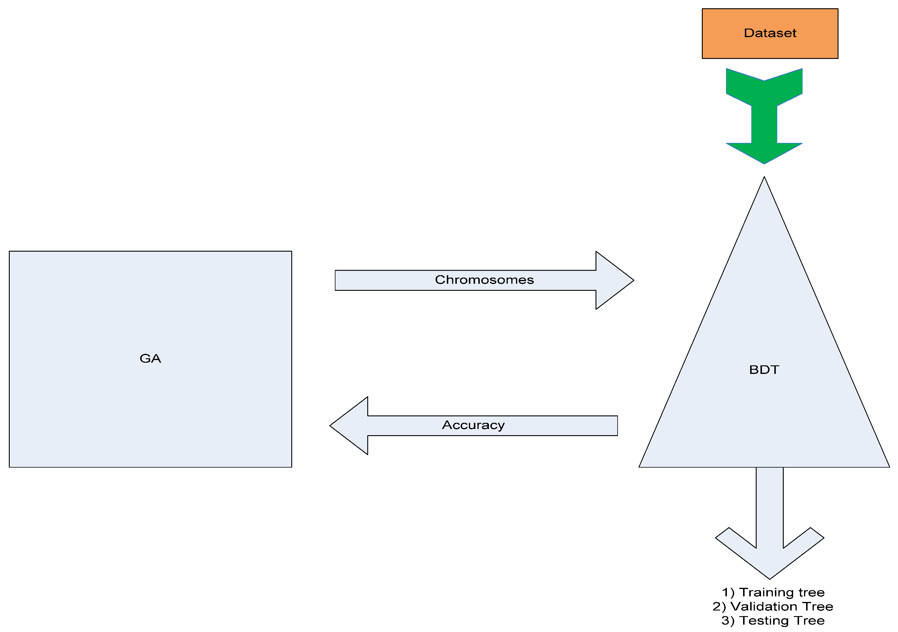
3.1. Method Overview

The goal of the selected method is to provide decision-makers with a tool that may process and evaluate large datasets, eliminating the risk of the decision. Due to computational power and complexity hybrid, the selected method is able to simultaneously handle data connections and perform tests. This study manages to examine the role of data and algorithms in providing efficient results in terms of accuracy for consumer behaviour predictions. The study’s final goal is to develop a method that can provide fast and accurate suggestions. The reason this application is important is because even if a DT is a widely used algorithm for classification problems, it still faces difficulties in data representation [12,13,14].

This method basically finds the attributes that participate the most in the classification process using a GA wrapper. It provides a novel approach to read, process, optimise, classify, and analyse data from a dataset. Feature selection methods are intended to reduce the number of input variables for those that are believed to be most useful to a model to predict the target variable. The two interconnected algorithms refer to a basic optimisation algorithm, the GA, and a basic classification non pruned algorithm, the binary DT (BDT). Both algorithms are wrapped together in a way that can be considered parallel data processing. The wrapping method can also be defined as the constant communicator between the GA and the DT algorithms. When a dataset is big, the classified data will be represented in a huge tree form. This tree is difficult to read and overfitting most probably occurs. To decrease the probability of this happening, the use of a GA is vital [15]. The logic behind the GA wrapper is on the grounds of selecting features from a dataset and sending them to the DTs for classification and tree representation each time. The GA is responsible for collecting and selecting the best subsets of features, which will perform equally as the initial number of features. Each time a subset of features arrives at the DTs, it is classified and assigned with a classification accuracy number, also called fitness, which denotes how effective the GA is in generating subsets [16]. This procedure is constantly repeated, and after a certain number of repetitions, the GA will return to the DT algorithm a combination of attributes that is represented as a tree structure. The wrapping method handles the entire communication between the DT and the GA and makes it seem like they are being executed simultaneously. By using this wrapping method and processing the data in parallel through the DT and the GA, overfitting is avoided. Moreover, a record can be generated of the best combination and the progress that has been achieved, and the classification of the data can be more easily represented. The best subset of attributes or genes is finally demonstrated through tree form representations, indicating the classification accuracy for training, validation, and testing sets of data [17,18].

3.2. Fitness Model

A crucial section of this study refers to the feature subset fitness evaluations and the method development. The fitness and accuracy numbers refer to the same value, which represents the efficiency of the GA wrapper to properly classify a set of features or chromosomes. For every generated chromosome, a classification process by the DTs algorithm takes place. The fitness is then sent to a GA and stored in a list of classified chromosomes. When the generated subsets of a generation are evaluated or classified, the best chromosomes participate in the creation of the next generation. Each chromosome has sixteen genes—fourteen genes refer to the class number and features and two more genes exist for extra class assignments (when an instance can be classified in more than one class). Depending on the goal of the experiments, the number of genes may be increased or reduced [19].

Accuracy calculation follows the process of every instance of the dataset, and it settles on the terminals of each BDT. The BDT consists of predicates and arithmetic symbols that make the calculations. The BDT reads the index of every instance, and it generates a number: the classification accuracy. The classification accuracy indicates the algorithm’s ability to predict the actual class of the subset or chromosome. There are occasions where a chromosome or instance may also belong in more than one class. After classifying all the available selected subsets or instances, each subset is assigned a value. These values refer to true positive if the instance is correctly classified from the BDT, which finally takes a vote. The performance of the best classification BDT that has contributed the most to the classification process is that with the biggest number of votes.

A classification of an instance is a result of the contribution of the entire BDTs population. The performance of each BDT is measured by the number of correct classification votes, while the number is a clear indicator of the best classifier. The number that shows the classification accuracy of an instance is measured by the fraction of the correctly classified instances upon the total number of the classified instances. Each instance classification accuracy number is stored in the GA, also called the fitness function, of the already classified chromosome. The fitness or accuracy value is stored in an array with the entire population of instances to be classified. The same process is followed during the classification stages of training, validation, and testing data. The classification accuracy or the maximum fitness and the fitness of the average chromosomes refer only to the population of the last generation, where the final and best results are generated. The validation and testing data that are used for model validation and testing purposes manage to perform equally in terms of classification accuracy or fitness number (Figure 1) [19].

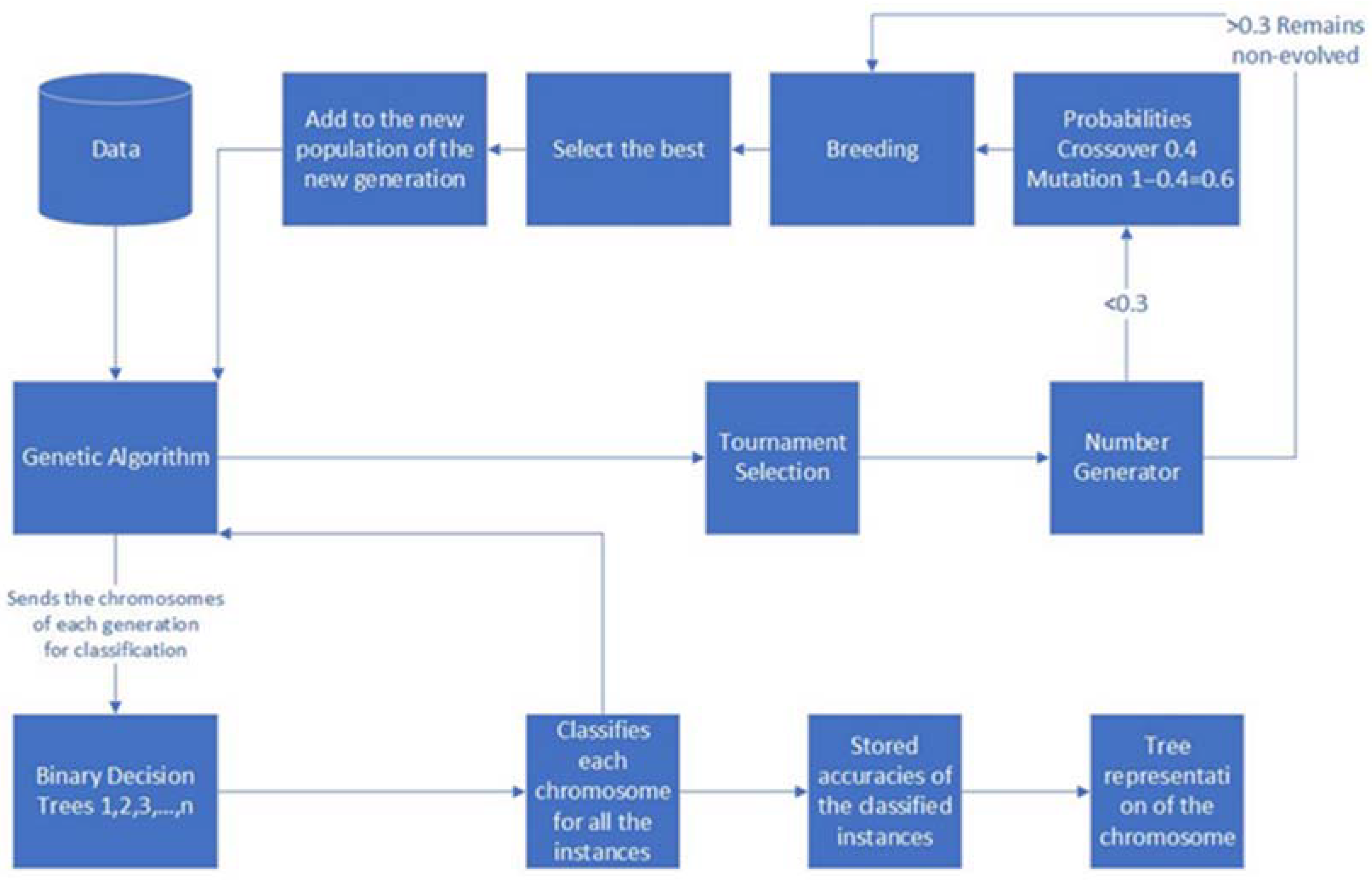
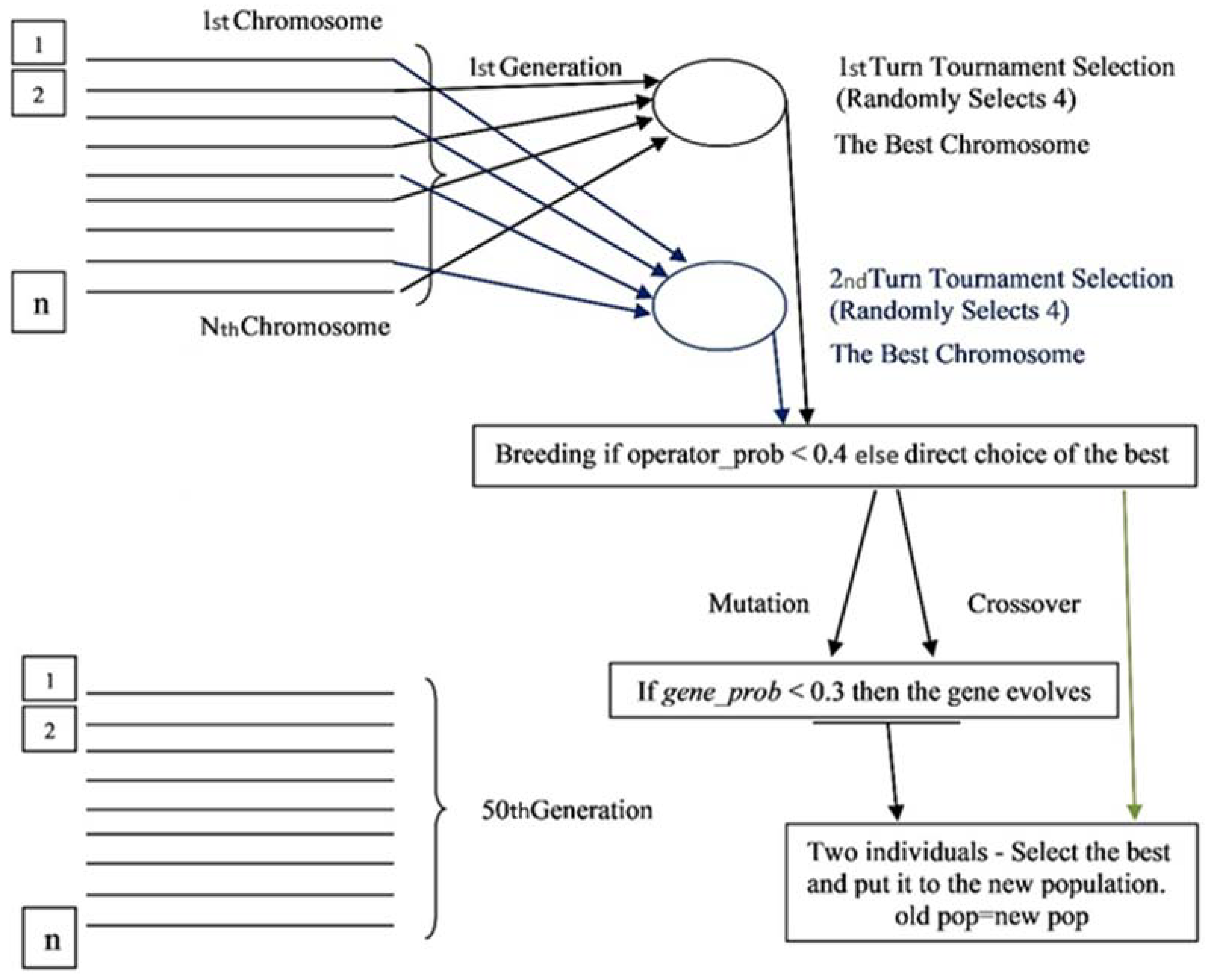
3.3. GA Wrapper Model Design

Information system diagrams are used to properly define the role and the design of the first level of this application. These information system diagrams describe how information is moving across the functions, indicating the procedures that contribute to the development. More specifically, in the current work, the use of flowcharts and sequence diagrams is considered essential for introducing the model to the reader. The flowchart, the abstract dataflow diagram, and the sequence diagram describe the backstage processes. The flowchart is a diagram that can show the basic functions of the entire project. It consists of the basic processes, the functions, and the messages that are sent among the different parts of the project. It explains how the genetic algorithm works and how the binary decision trees are associated with the genetic algorithm. The wrapping method is a part of the implementation, and it cannot be demonstrated separately from the entire application (Figure 2) [20]. The genetic algorithm reads the attributes of the dataset and starts to randomly create the population of chromosomes of the first generation. Some of the chromosomes may have the same attributes as genes more than one time. In order to create the rest of the generations, the tournament selection method, the mutation, the crossover, and the selection of the best method are used (Figure 3) [20,21].

3.4. GA Wrapper Analysis

The tournament variable refers to the previously mentioned tournament selection. According to the tournament selection, on the first run, the algorithm randomly chooses a specific number of chromosomes from the entire population. The user indicates the number of chromosomes by assigning the variable tournament a number (e.g., tournament = 4). From this number of chromosomes, the GA picks the chromosome with the biggest fitness number. It remains in the first generation and the tournament runs again until a set of 100 chromosomes is complete for the 1st generation. The tournament selection is used instead of the roulette selection in this work. As soon as two chromosomes are picked from the first two runs, the procedures of mutation or crossover may take place in order to produce two new chromosomes (Figure 3) [21].

The variable that decides if a gene is going to be changed is the gene probability (gene_prob). The value of the gene_prob is set to 0.3. If the generator produces a smaller number, then the specific gene will be evolved. There is a variable that decides if the genes of the first two selected as the best chromosomes will be mutated or crossover-ed. This variable is the operator probability (operator_prob) that randomly generates numbers. If the generated number is less than <0.4, then the procedure of the mutation or crossover will take place. The possibility of a crossover taking place is 40% and the probability of mutation is 60%. Out of these two chromosomes, the best is chosen and stored in an array. When the array is filled with 100 evolved or not evolved chromosomes, the second generation is created. The next generations are created in the same way as the second. The generation variable defines the number of the generations, and the population variable can also take different values by the user and defines the size of the population of the chromosomes of each generation. The operator_prob and the gene_prob can change by the user (Figure 3) [21].

The first plan for the decision tree algorithm was to build the application according to the original decision tree theory which includes the information gain and Shannon function mathematic formulas. Instead of using the standard decision tree algorithm, another decision tree is used, known as the binary decision tree or the ensemble full binary decision trees. A full binary decision tree is a symmetric, fully deployed tree with all of its nodes reaching the terminals. The tree has a depth of 4. There is a variable in the code declared as maximum decision trees (max_dt) and it defines the number of DTs that are constructed and participate in the classification process. The sizes of the trees are fixed, and the user can change the number. Suppose the max_dt is 10—this means that 10 decision trees are created and all of them contribute to the classification (Figure 3) [21,22].

The datasets are separated into three parts. The training set, the validation set, and an additional check, the testing set. The training set trains the model and the validation set validates the already trained examples of the training set. After the training of the program, the validation set checks again all the results with new data. After validating the test results using the validation data, there is another fraction of data called the testing set that is used to validate only the result with the biggest accuracy of all the validated results. The dataset is usually split into the training set with the 50%, the validation set with the 20%, and the testing set with the 30% of all the examples [22].

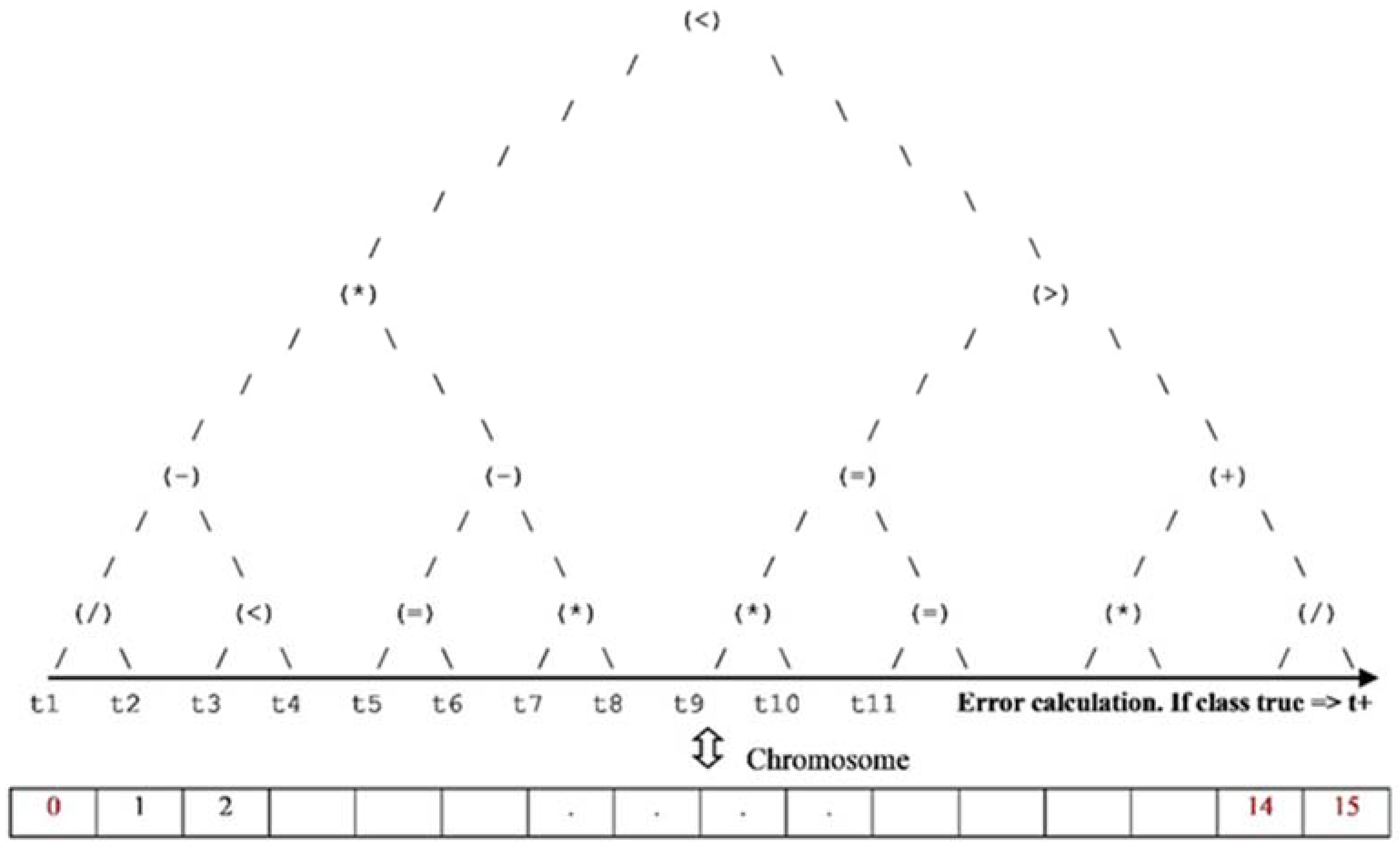
3.5. GA Wrapper Chromosome Representation

The tree with the biggest number of votes is represented. There are three types of represented trees. The 1st is the dominant training tree, which classifies the training data. The 2nd is the dominant validation tree, where the classification of only the previous one’s population’s validation data takes place. The 3rd is the dominant testing tree, where the classification of only the former’s population’s testing data takes place (Figure 4).

3.6. Dataset

The current data is extracted from a questionnaire that is used to examine consumers’ behaviour during the pandemic in Greece. Out of 1882 questionnaires, 1603 were usable. Three different independent variables were examined for good attribute subsets selection: Gender (classes 1,2), Household’s Size (classes 1,2,3,4,5), and Household’s Monthly Income (classes 1,2,3,4,5). The variables refer to 13 questions (

Table 1. Consumers Dataset.

Position	Genes	Description	Value	Label
0 (Class)	v1	Gender	Male	1
			Female	2
0 (Class)	v2	Household’s Size	1	1
			2	2
			3	3
			4	4
			>=5	5
0 (Class)	v4	Household’s Monthly Income	<500.00 €	1
			501.00–1000.00 €	2
			1001.00–1500.00 €	3
			1501.00–2000.00 €	4
			>2001.00 €	5
1	v5	When you find Greek products in the supermarkets do you prefer them over the imported products from abroad?	Yes	1
			No	2
2	v6	During the health crisis (today) do you prefer Greek products more than before?	Yes	1
			No	2
			Same As Before	3
3	v7	Do you want the companies from which you choose to make some of your purchases to inform you in detail about the measures they have taken regarding coronavirus protection?	Yes	1
			No	2
4	v8	After the health crisis, things will return to normal relatively quickly	Abs Disagree	1
			Disagree	2
			Neutral	3
			Agree	4
			Abs Agree	5
5	v9	After the health crisis, social life will be the same as before	Abs Disagree	1
			Disagree	2
			Neutral	3
			Agree	4
			Abs Agree	5
6	v11	During the health crisis my family makes savings efforts	Abs Disagree	1
			Disagree	2
			Neutral	3
			Agree	4
			Abs Agree	5
7	v13	The health crisis has affected the way we purchase	Abs Disagree	1
			Disagree	2
			Neutral	3
			Agree	4
			Abs Agree	5
8	v14	During the health crisis the quantities we buy from the Super Markets have increased	Abs Disagree	1
			Disagree	2
			Neutral	3
			Agree	4
			Abs Agree	5
9	v15	The health crisis has boosted online shopping	Abs Disagree	1
			Disagree	2
			Neutral	3
			Agree	4
			Abs Agree	5
10	v17	We buy more from brands that have offers during this period	Abs Disagree	1
			Disagree	2
			Neutral	3
			Agree	4
			Abs Agree	5
11	v18	During the health crisis we have started trying new brands	Abs Disagree	1
			Disagree	2
			Neutral	3
			Agree	4
			Abs Agree	5
12	v20	Do you buy more sparsely or more often compared to the pre-coronavirus era?	Less Frequently	1
			The Same	2
			More Frequently	3
13	v22	Approximately how much money do you spend every time you shop at the supermarkets now that we have a coronavirus problem (today)?	<50 €	1
			≈50 €	2
			>50 €	3
			>100 €	4

) [23].

4. Results

In this part, GA wrapper performance is tested on consumer data. Primarily, the objective is to test whether the GA wrapper adequately performs in different contexts and, secondly, to predict which factors will affect consumer behaviours. The parameters are set in Section 3.4. The experiments include the three best runs. The results are displayed in the form Generation (Number) = Average Fitness (Best Fitness).

4.1. Average and Best Generation Fitness

4.1.1. Best Fitness

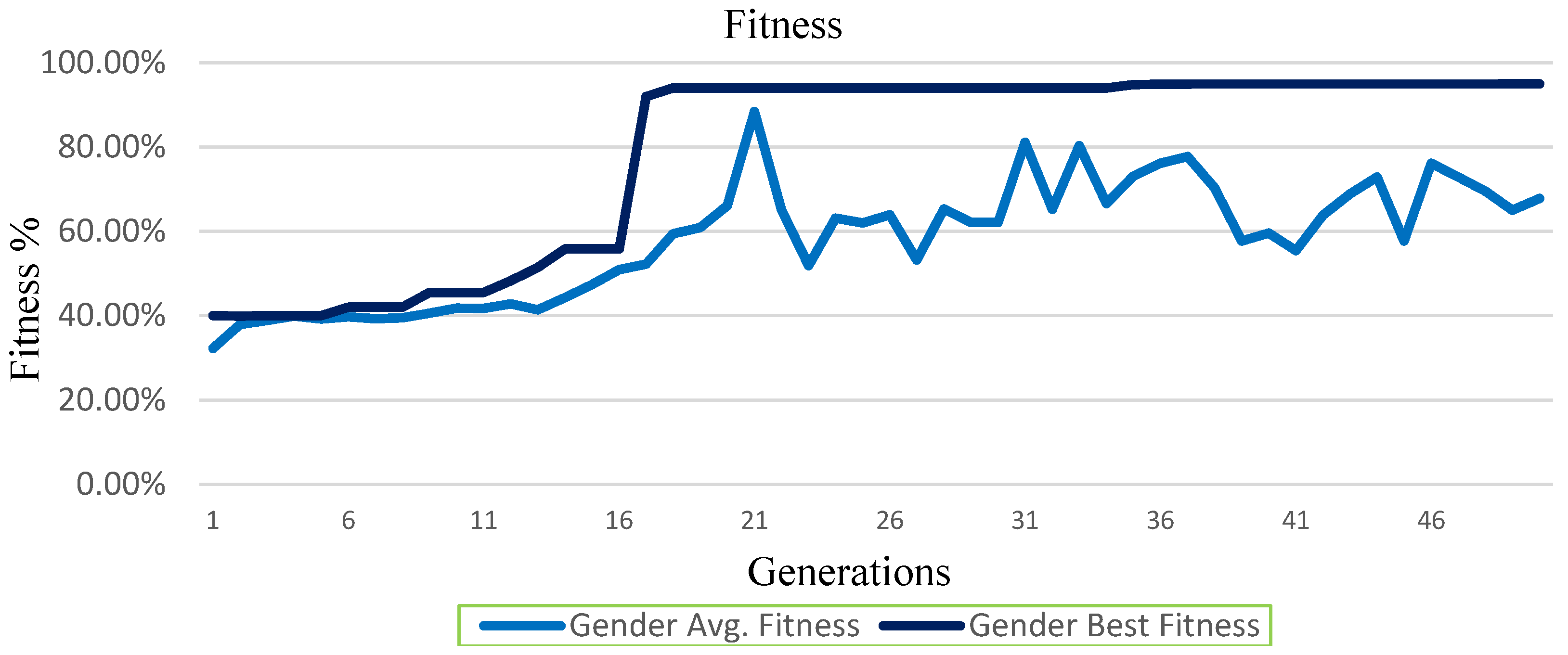
• Gender classification problem solved at the highest rate of Training Fitness = 95.00%, Validation Fitness = 95.30%, Testing Fitness = 92.50% (

  Table 2. Average and Best Generation Fitness for Gender.

  Gender Generation Fitness
  Generation	Avg. Fitness	Best Fitness	Generation	Avg. Fitness	Best Fitness
  Generation 0	0.323	0.400	Generation 25	0.639	0.940
  Generation 1	0.379	0.399	Generation 26	0.532	0.940
  Generation 2	0.389	0.400	Generation 27	0.653	0.940
  Generation 3	0.399	0.400	Generation 28	0.621	0.940
  Generation 4	0.392	0.400	Generation 29	0.621	0.940
  Generation 5	0.397	0.420	Generation 30	0.811	0.940
  Generation 6	0.393	0.420	Generation 31	0.652	0.940
  Generation 7	0.395	0.420	Generation 32	0.803	0.940
  Generation 8	0.406	0.455	Generation 33	0.666	0.940
  Generation 9	0.418	0.455	Generation 34	0.731	0.948
  Generation 10	0.417	0.455	Generation 35	0.761	0.950
  Generation 11	0.428	0.483	Generation 36	0.777	0.950
  Generation 12	0.414	0.514	Generation 37	0.703	0.950
  Generation 13	0.443	0.558	Generation 38	0.577	0.950
  Generation 14	0.474	0.558	Generation 39	0.596	0.950
  Generation 15	0.509	0.558	Generation 40	0.554	0.950
  Generation 16	0.522	0.919	Generation 41	0.638	0.950
  Generation 17	0.594	0.940	Generation 42	0.689	0.950
  Generation 18	0.609	0.940	Generation 43	0.729	0.950
  Generation 19	0.661	0.940	Generation 44	0.577	0.950
  Generation 20	0.884	0.940	Generation 45	0.761	0.950
  Generation 21	0.651	0.940	Generation 46	0.729	0.950
  Generation 22	0.519	0.940	Generation 47	0.695	0.950
  Generation 23	0.631	0.940	Generation 48	0.650	0.950
  Generation 24	0.620	0.940	Generation 49	0.678	0.950

  );
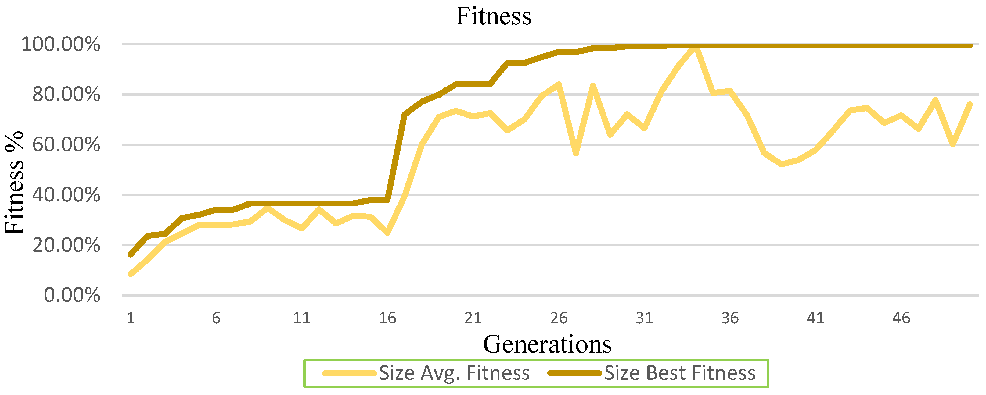
• Household size classification problem solved at the highest rate of Training Fitness = 99.70%, Validation Fitness = 99.70%, Testing Fitness = 99.80% (

  Table 3. Best Generation Fitness for Household Size.

  Household Size Generation Fitness
  Generation	Avg. Fitness	Best Fitness	Generation	Avg. Fitness	Best Fitness
  Generation 0	0.084	0.163	Generation 25	0.840	0.969
  Generation 1	0.143	0.237	Generation 26	0.566	0.969
  Generation 2	0.212	0.244	Generation 27	0.834	0.984
  Generation 3	0.246	0.307	Generation 28	0.640	0.984
  Generation 4	0.280	0.321	Generation 29	0.721	0.992
  Generation 5	0.281	0.341	Generation 30	0.666	0.992
  Generation 6	0.282	0.341	Generation 31	0.813	0.994
  Generation 7	0.294	0.366	Generation 32	0.915	0.997
  Generation 8	0.348	0.366	Generation 33	0.996	0.997
  Generation 9	0.300	0.366	Generation 34	0.806	0.997
  Generation 10	0.266	0.366	Generation 35	0.814	0.997
  Generation 11	0.342	0.366	Generation 36	0.717	0.997
  Generation 12	0.286	0.366	Generation 37	0.567	0.997
  Generation 13	0.316	0.366	Generation 38	0.521	0.997
  Generation 14	0.313	0.380	Generation 39	0.539	0.997
  Generation 15	0.249	0.380	Generation 40	0.579	0.997
  Generation 16	0.394	0.719	Generation 41	0.655	0.997
  Generation 17	0.600	0.771	Generation 42	0.736	0.997
  Generation 18	0.710	0.799	Generation 43	0.746	0.997
  Generation 19	0.735	0.841	Generation 44	0.687	0.997
  Generation 20	0.712	0.841	Generation 45	0.716	0.997
  Generation 21	0.726	0.842	Generation 46	0.663	0.997
  Generation 22	0.657	0.926	Generation 47	0.777	0.997
  Generation 23	0.701	0.926	Generation 48	0.602	0.997
  Generation 24	0.794	0.949	Generation 49	0.760	0.997

  );
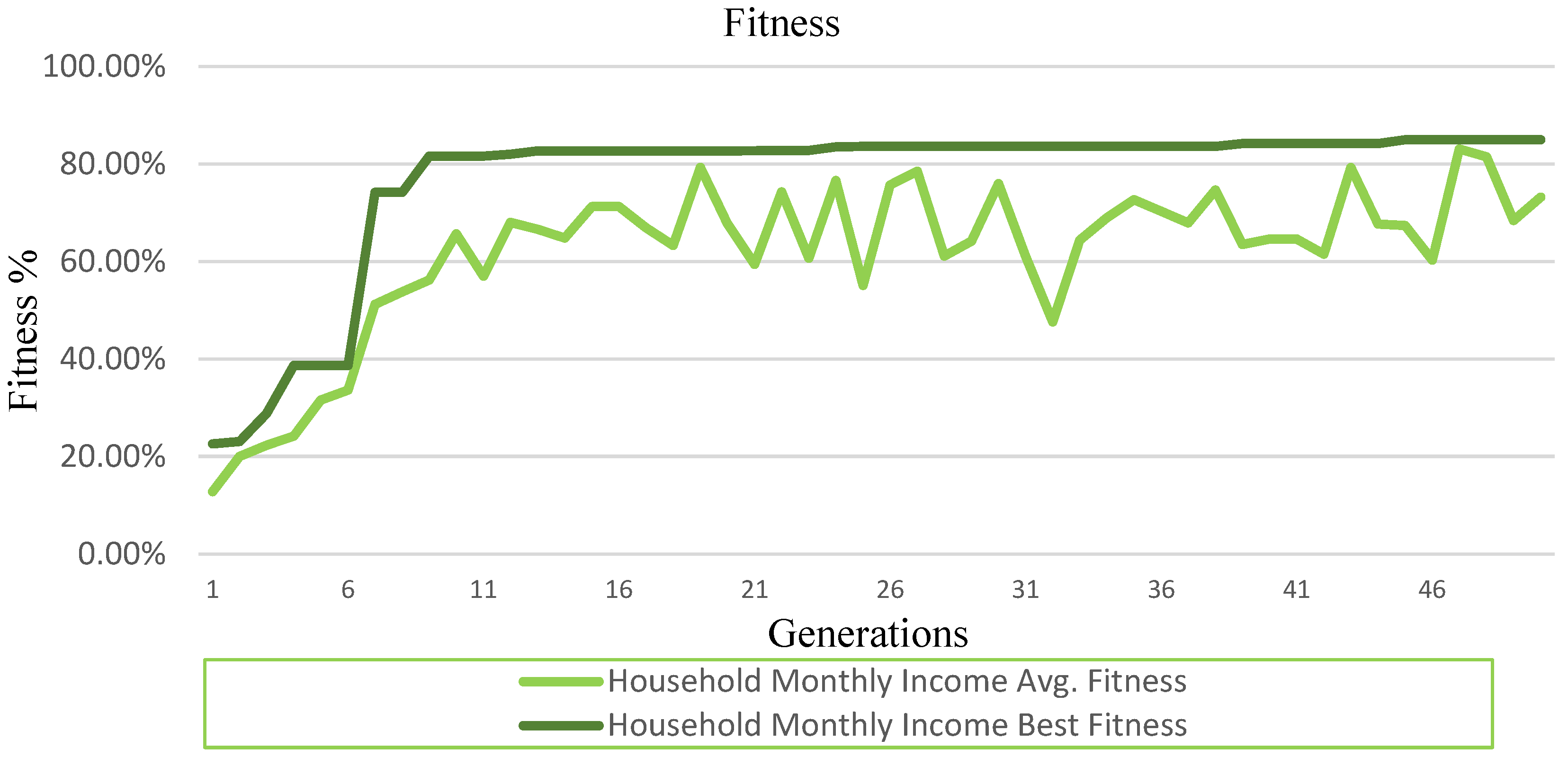
• Household Monthly Income classification problem solved at the highest rate of Training Fitness = 85.00%, Validation Fitness = 85.80%, Testing Fitness = 86.50% (

  Table 4. Best Generation Fitness for Household Monthly Income.

  Household Monthly Income Generation Fitness
  Generation	Avg. Fitness	Best Fitness	Generation	Avg. Fitness	Best Fitness
  Generation0	0.128	0.226	Generation 25	0.757	0.836
  Generation 1	0.200	0.231	Generation 26	0.785	0.836
  Generation 2	0.223	0.288	Generation 27	0.611	0.836
  Generation 3	0.242	0.387	Generation 28	0.642	0.836
  Generation 4	0.316	0.387	Generation 29	0.760	0.836
  Generation 5	0.336	0.387	Generation 30	0.611	0.836
  Generation 6	0.512	0.742	Generation 31	0.476	0.836
  Generation 7	0.538	0.742	Generation 32	0.644	0.836
  Generation 8	0.562	0.816	Generation 33	0.690	0.836
  Generation 9	0.657	0.816	Generation 34	0.727	0.836
  Generation 10	0.570	0.816	Generation 35	0.703	0.836
  Generation 11	0.680	0.820	Generation 36	0.679	0.836
  Generation 12	0.666	0.827	Generation 37	0.747	0.836
  Generation 13	0.648	0.827	Generation 38	0.635	0.842
  Generation 14	0.713	0.827	Generation 39	0.646	0.842
  Generation 15	0.713	0.827	Generation 40	0.646	0.842
  Generation 16	0.669	0.827	Generation 41	0.615	0.842
  Generation 17	0.633	0.827	Generation 42	0.793	0.842
  Generation 18	0.793	0.827	Generation 43	0.677	0.842
  Generation 19	0.678	0.827	Generation 44	0.674	0.850
  Generation 20	0.594	0.827	Generation 45	0.603	0.850
  Generation 21	0.743	0.828	Generation 46	0.831	0.850
  Generation 22	0.607	0.828	Generation 47	0.815	0.850
  Generation 23	0.766	0.835	Generation 48	0.684	0.850
  Generation 24	0.551	0.836	Generation 49	0.732	0.850

  ).

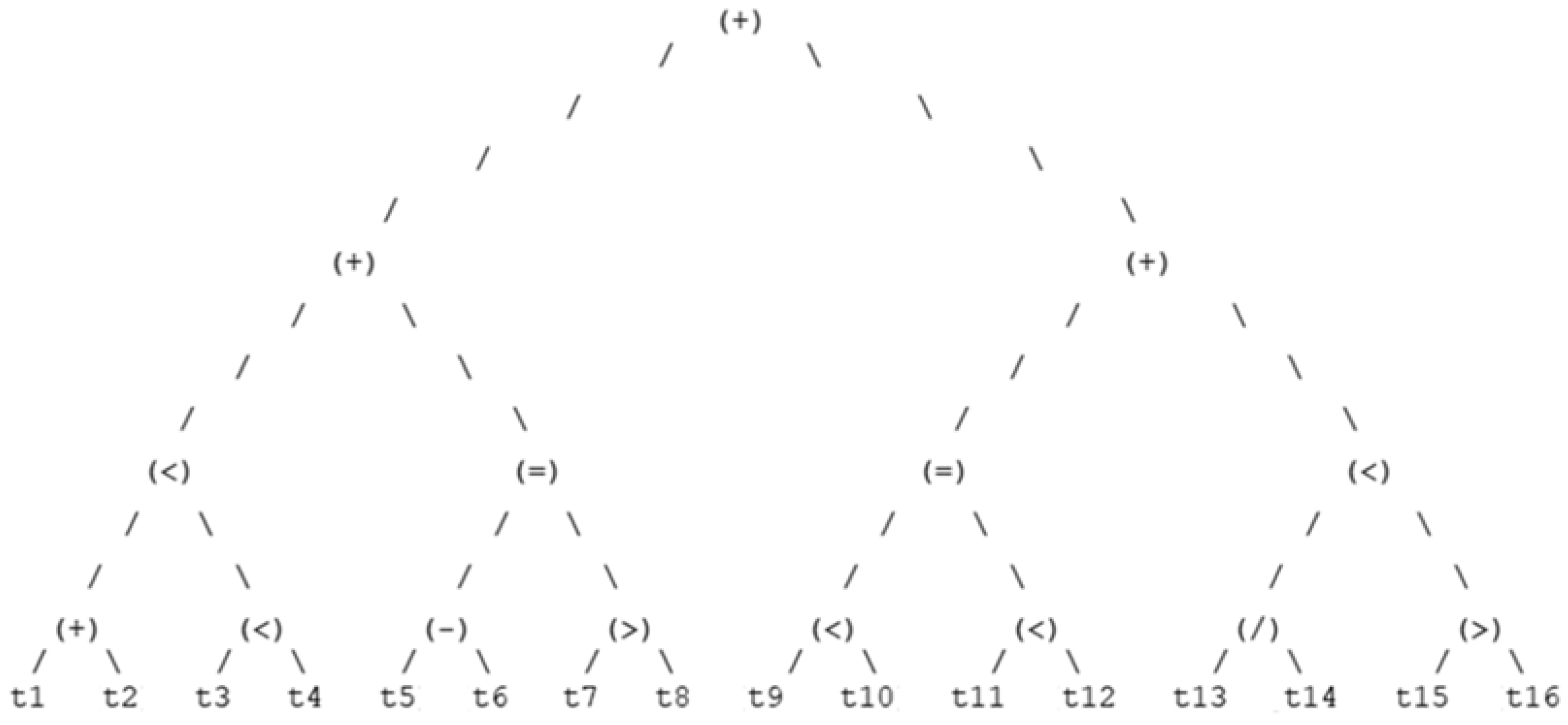
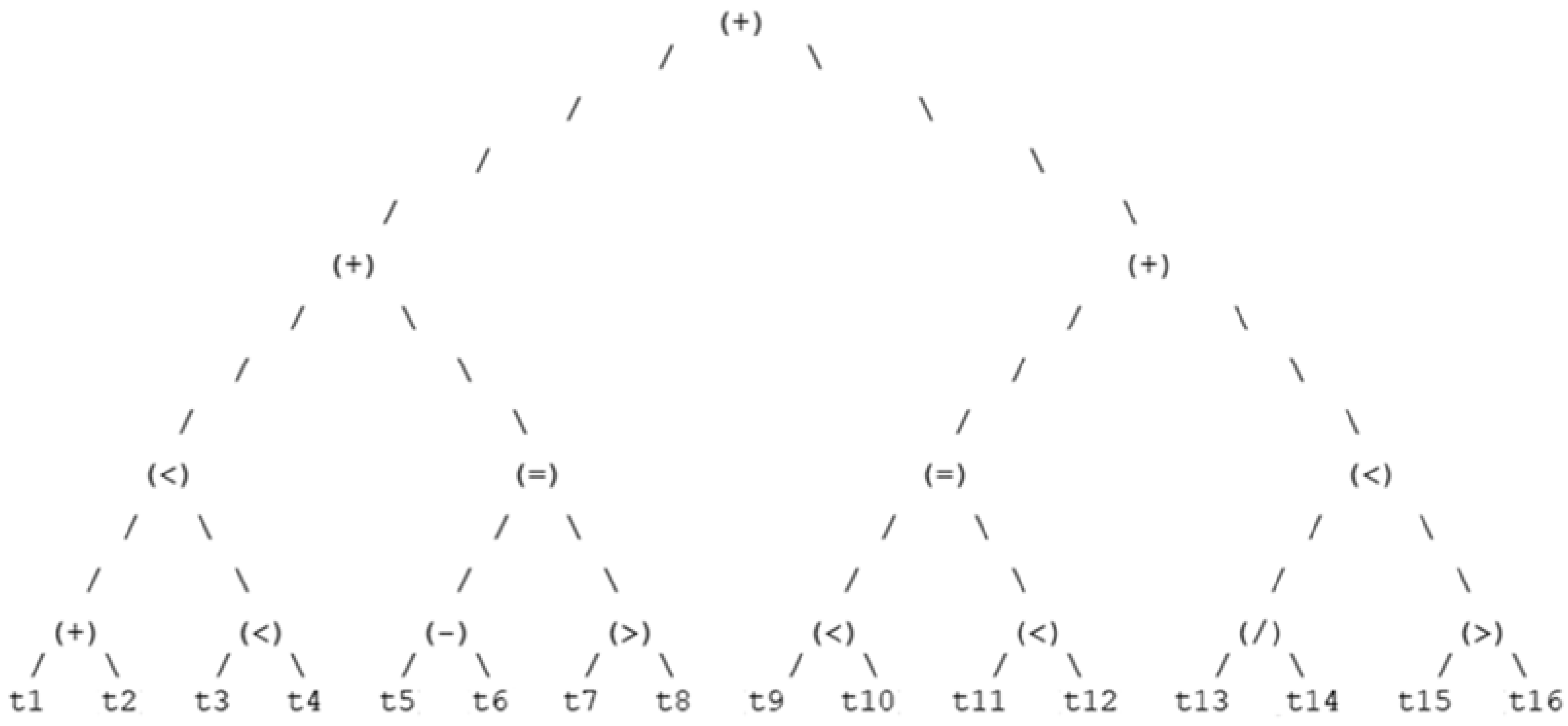
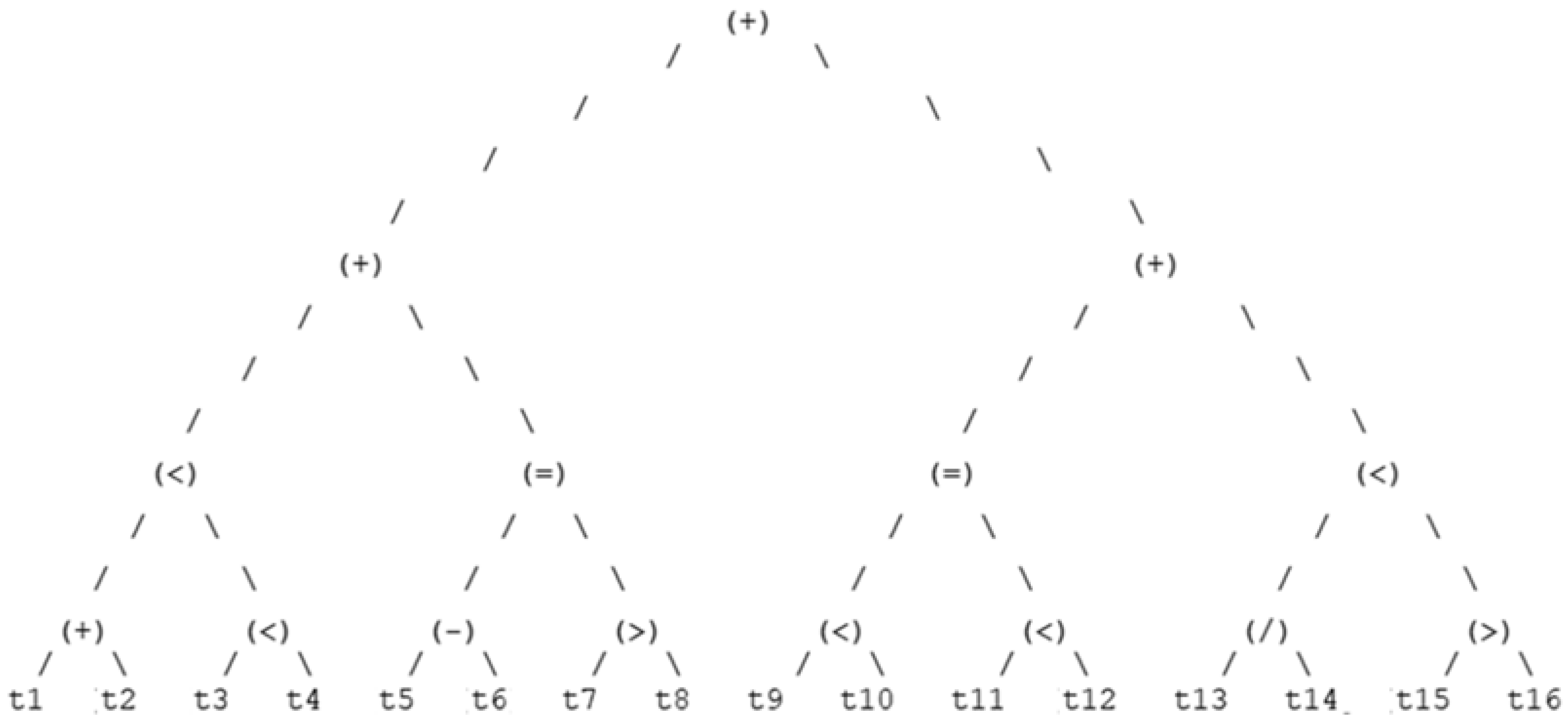
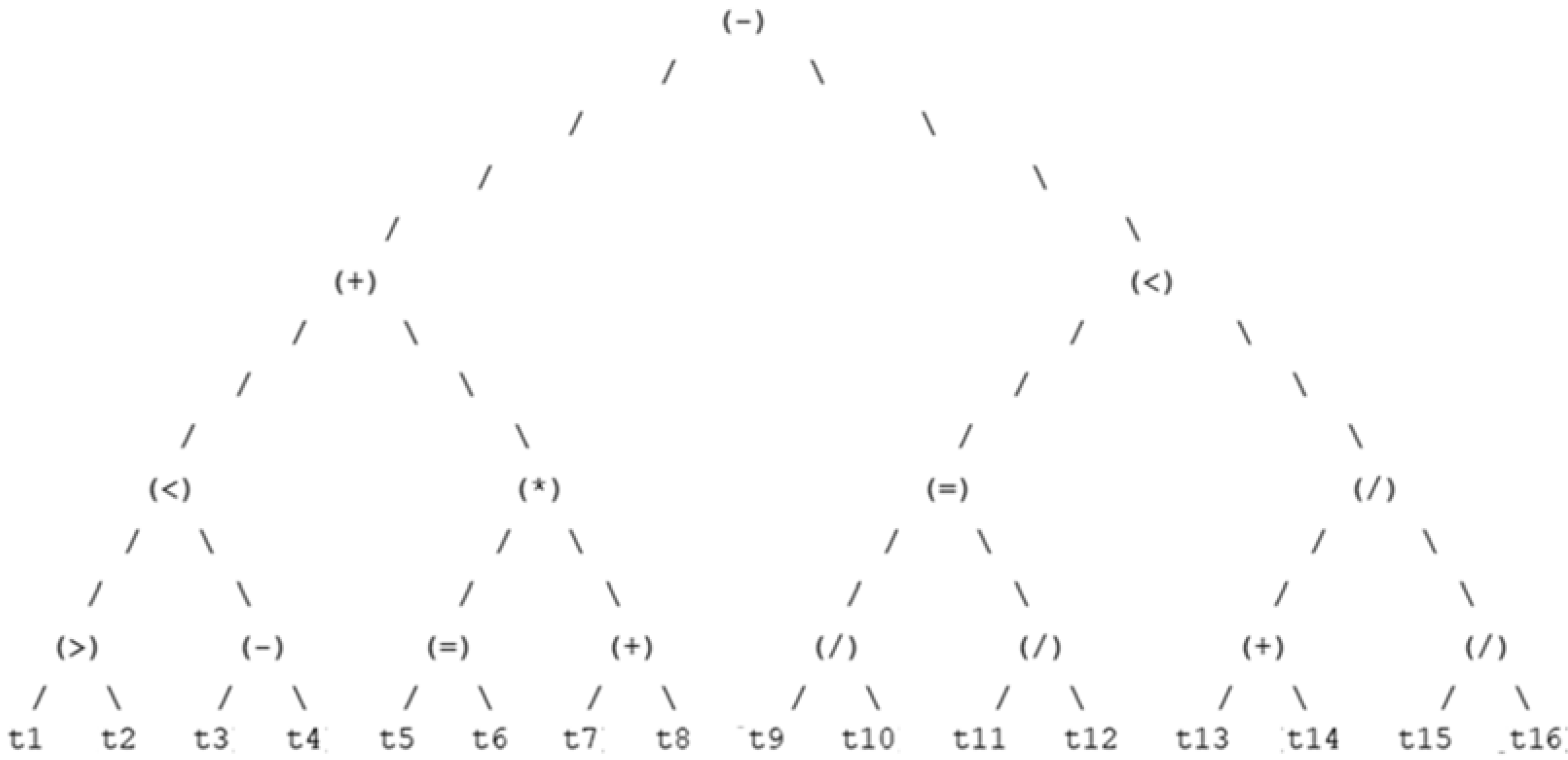
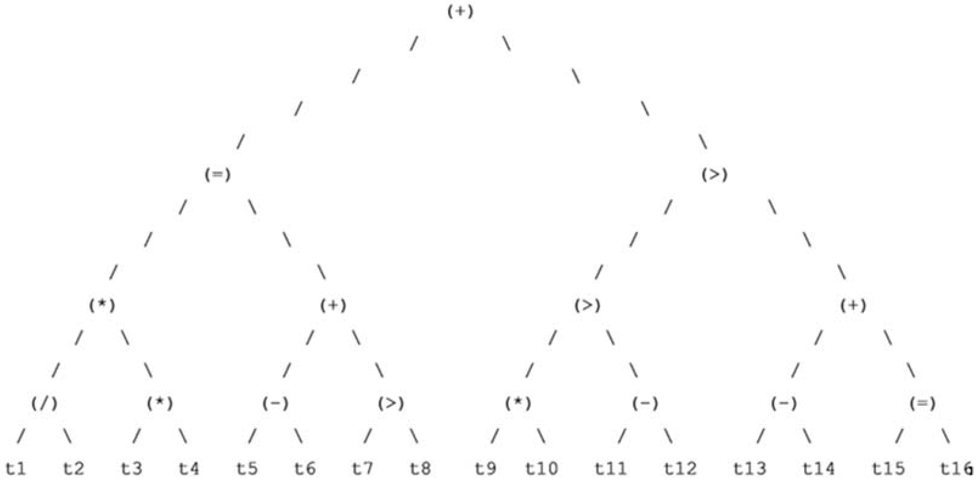
4.1.2. Optimal Decision Trees

This part shows the decision trees, which have contributed the most to the classification for gender, household size, and household monthly income. There are 10 DTs for the training set, 10 DTs for the validation set, and 10 DTs for the testing set. Each tree from 0 to 9 has a number that indicates the votes it takes for every correct classification. The maximum (MAX) votes highlight the tree with the biggest number of votes and this tree is finally going to be represented.

The rest of the trees have also contributed to a better classification, but they are not represented. The results are displayed in the form of Decision Tree (Number) = Number of Votes (

Table 5. Optimal Decision Trees for Gender Classification.

Training Votes	Validation Votes	Testing Votes
Tree (0) = 933	Tree (0) = 0	Tree (0) = 0
Tree (1) = 263,126	Tree (1) = 236	Tree (1) = 16
Tree (2) = 58,444	Tree (2) = 0	Tree (2) = 0
Tree (3) = 70,777	Tree (3) = 44	Tree (3) = 0
Tree (4) = 3,023,415	Tree (4) = 2656 MAX	Tree (4) = 263 MAX
Tree (5) = 2580	Tree (5) = 0	Tree (5) = 0
Tree (6) = 28,321	Tree (6) = 0	Tree (6) = 0
Tree (7) = 422,696	Tree (7) = 12	Tree (7) = 0
Tree (8) = 882,731	Tree (8) = 1288	Tree (8) = 0
Tree (9) = 4,503,777 MAX	Tree (9) = 2484	Tree (9) = 202

,

Table 6. Optimal Decision Trees for Household Size Classification.

Training Votes	Validation Votes	Testing Votes
Tree (0) = 6,000,732 MAX	Tree (0) = 4827 MAX	Tree (0) = 454 MAX
Tree (1) = 452,433	Tree (1) = 185	Tree (1) = 6
Tree (2) = 66,823	Tree (2) = 252	Tree (2) = 0
Tree (3) = 14,962	Tree (3) = 0	Tree (3) = 0
Tree (4) = 1,437,664	Tree (4) = 418	Tree (4) = 0
Tree (5) = 124,103	Tree (5) = 14	Tree (5) = 0
Tree (6) = 169,510	Tree (6) = 164	Tree (6) = 0
Tree (7) = 102,219	Tree (7) = 168	Tree (7) = 0
Tree (8) = 145,125	Tree (8) = 72	Tree (8) = 0
Tree (9) = 720,087	Tree (9) = 578	Tree (9) = 21

and

Table 7. Optimal Decision Trees for Household Monthly Income Classification.

Training Votes	Validation Votes	Testing Votes
Tree (0) = 6,582,160 MAX	Tree (0) = 5444 MAX	Tree (0) = 429 MAX
Tree (1) = 80,157	Tree (1) = 0	Tree (1) = 0
Tree (2) = 8805	Tree (2) = 8	Tree (2) = 0
Tree (3) = 11,732	Tree (3) = 42	Tree (3) = 0
Tree (4) = 61,907	Tree (4) = 2	Tree (4) = 3
Tree (5) = 502,862	Tree (5) = 18	Tree (5) = 3
Tree (6) = 1662	Tree (6) = 0	Tree (6) = 0
Tree (7) = 208,654	Tree (7) = 56	Tree (7) = 0
Tree (8) = 457,921	Tree (8) = 371	Tree (8) = 3
Tree (9) = 1,317,798	Tree (9) = 695	Tree (9) = 45

).

4.1.3. Dominant Decision Trees Representation

Figure 5, Figure 6, Figure 7, Figure 8, Figure 9, Figure 10, Figure 11, Figure 12 and Figure 13 show the dominant training, validation, and testing binary decision trees for all the Gender, Household Size, and Household Monthly Income classes. They represent the structure of each of the selected dominant DTs for all the independent variables. The dominant decision trees refer to those who get the biggest number of votes during the classification process.

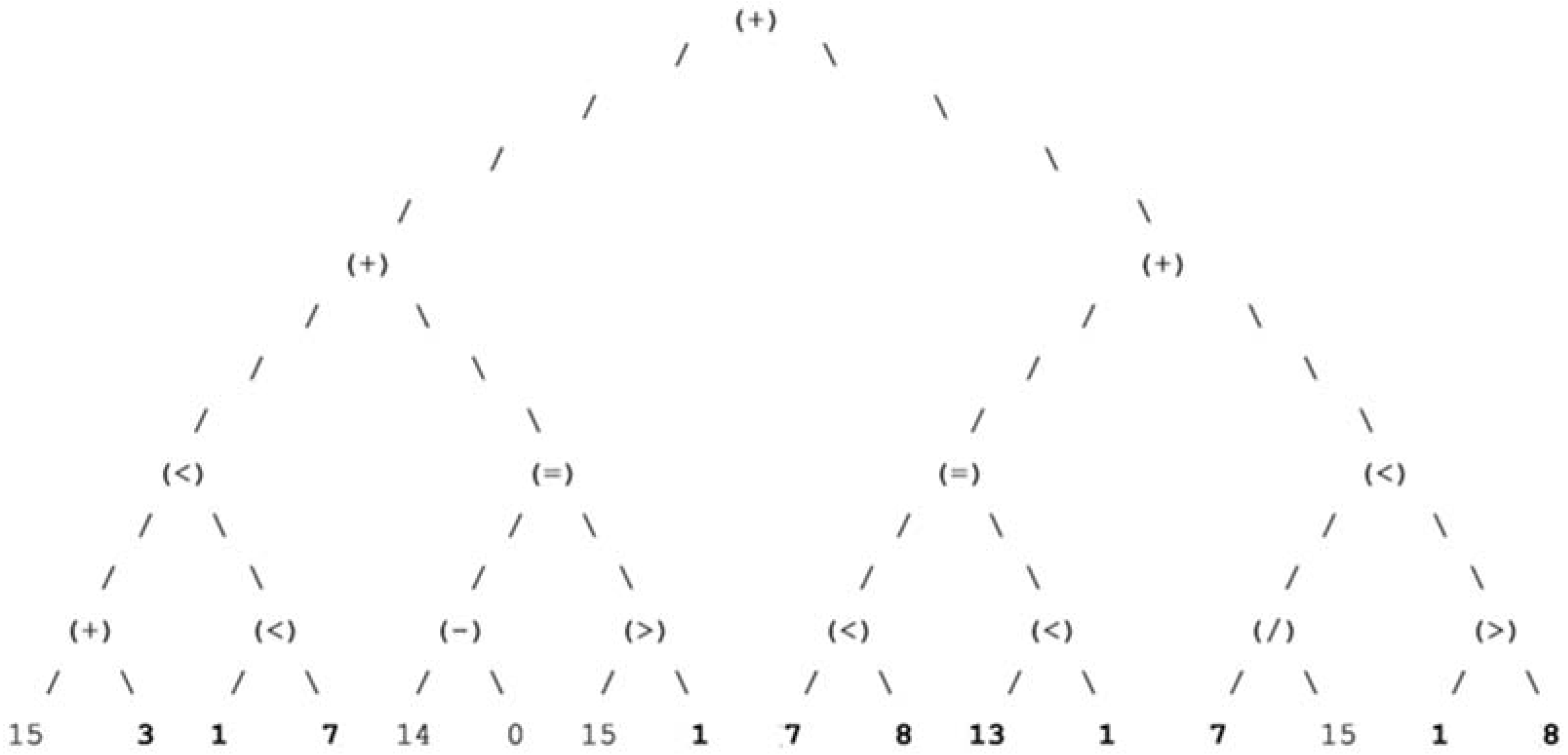
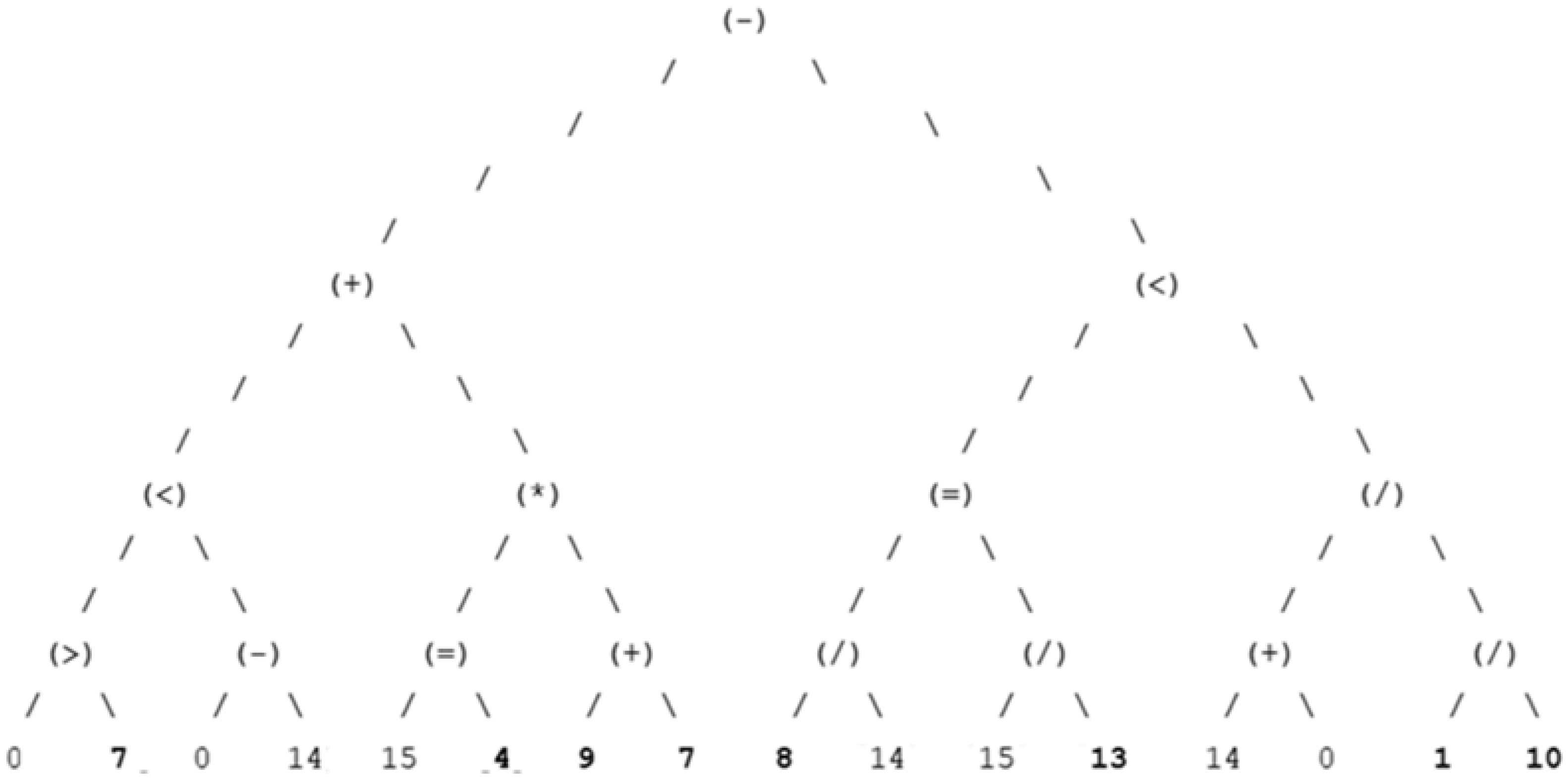
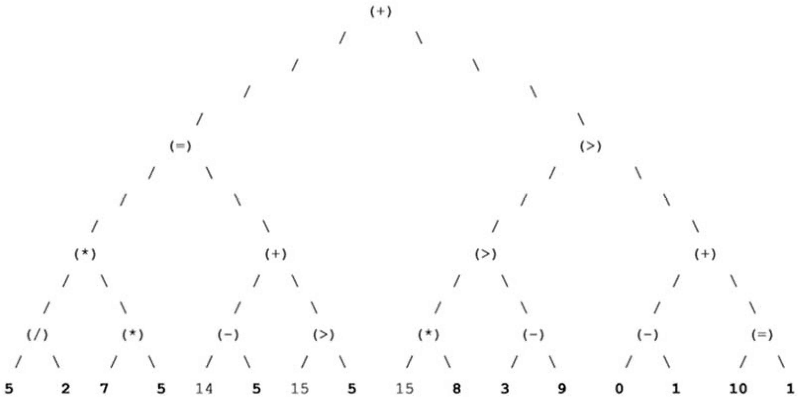
4.1.4. Best Chromosome Sequence & Decision Tree Representation

Following the final structure of the most dominant DTs, Figure 14, Figure 15 and Figure 16 and

Table 8. Best Chromosome Gene Frequency for Class Gender.

Gene Position	Gene Tag (Attribute)	Occurence
0	v1 Class {1,2}	1
1	v5	4
3	v7	1
7	v13	3
8	v14	2
13	v22	1

,

Table 9. Best Chromosome Gene Frequency for Class Household Size.

Gene Position	Gene Tag (Attribute)	Occurence
0	v1 Class {1,2,3,4,5}	3
1	v5	1
4	v8	1
7	v13	2
8	v14	1
9	v15	1
10	v17	1
13	v22	1

and

Table 10. Best Chromosome Gene Frequency for Class Household Monthly Income.

Gene Position	Gene Tag (Attribute)	Occurence
0	v1 Class {1,2,3,4,5}	1
1	v5	2
2	v6	1
3	v7	1
5	v9	4
7	v13	1
8	v14	1
9	v15	1
10	v17	1

show how the dominant genes can be classified. The dominant testing trees are demonstrated by applying the last generation’s testing gene population. They demonstrate the best chromosomes, including the genes (attributes) that mostly participated in the classification process:

• Gender elitist chromosome: (15) (3) (1) (7) (14) (0) (15) (1) (7) (8) (13) (1) (7) (15) (1) (8)—92.5% Fitness;
• Household Size elitist chromosome: (0) (7) (0) (14) (15) (4) (9) (7) (8) (14) (15) (13) (14) (0) (1) (10)—99.8% Fitness;
• Household Monthly Income elitist chromosome: (5) (2) (7) (5) (14) (5) (15) (5) (15) (8) (3) (9) (0) (1) (10) (1)—86.5% Fitness.

4.1.5. Classification Fitness Graphical Representation

The blue lines indicate the average and the best fitness of the Gender chromosomes. The yellow lines indicate the average and the best fitness of the Household Size chromosomes. The green lines indicate the average and the best fitness of the Household Monthly Income chromosomes (Figure 17, Figure 18 and Figure 19).

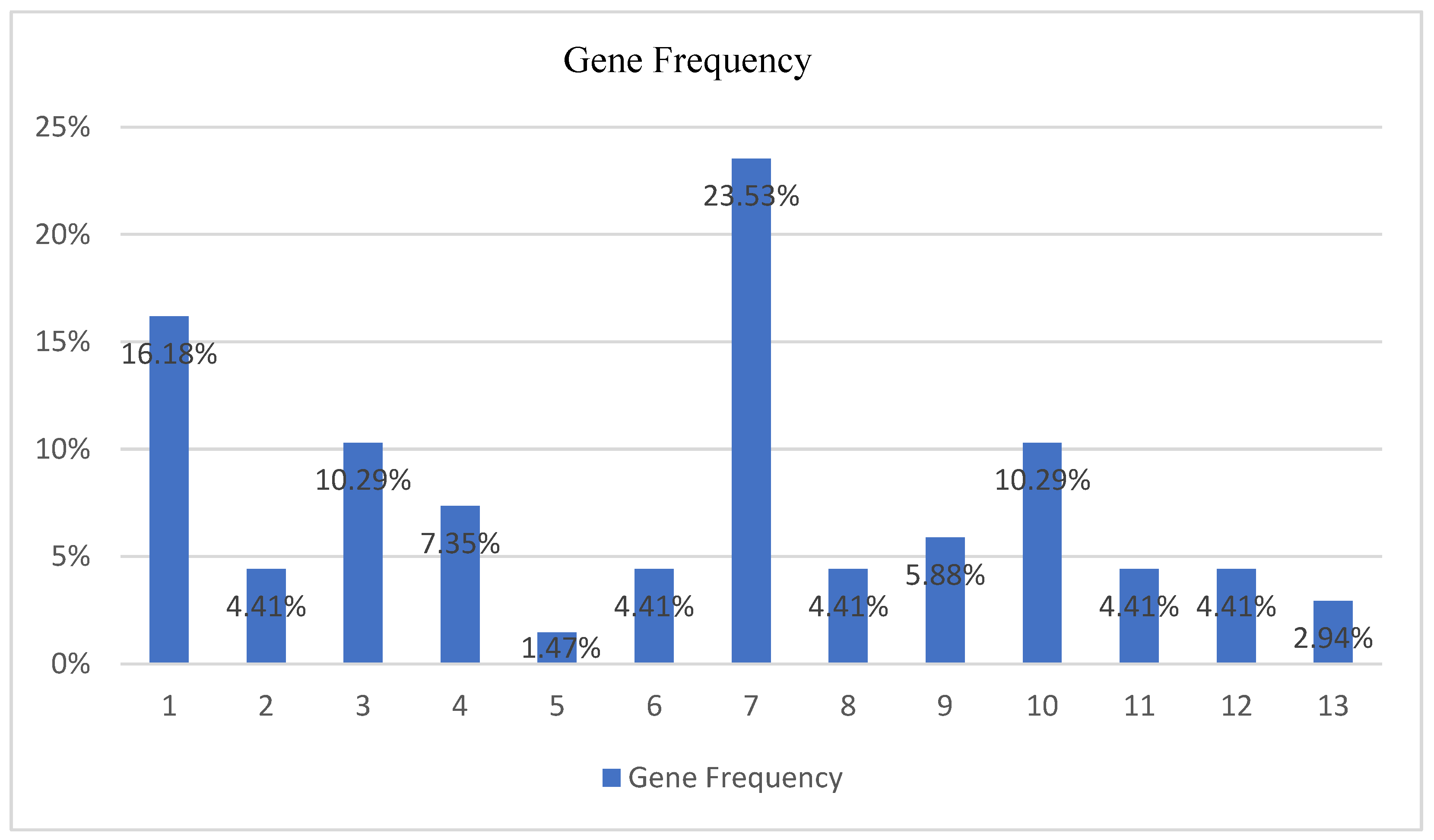
4.1.6. Average Genes Frequency

Table 11. Genes Average Frequency for the Gender.

	Runs No							Genes Average Frequency of Occurrence
Gene	1	2	3	4	5	6	7	Avg Occurrence	Avg Occurrence%
1	4	2	0	0	1	3	1	1.571429	16.18%
2	0	2	1	0	0	0	0	0.428571	4.41%
3	1	1	0	4	0	1	0	1	10.29%
4	0	1	0	0	0	2	2	0.714286	7.35%
5	0	0	1	0	0	0	0	0.142857	1.47%
6	0	0	0	0	1	0	2	0.428571	4.41%
7	3	0	3	6	1	2	1	2.285714	23.53%
8	2	0	1	0	0	0	0	0.428571	4.41%
9	0	0	1	0	1	1	1	0.571429	5.90%
10	0	2	1	0	4	0	0	1	10.29%
11	0	0	0	1	1	0	1	0.428571	4.41%
12	0	2	0	1	0	0	0	0.428571	4.41%
13	1	0	0	0	0	0	1	0.285714	2.94%

,

Table 12. Genes Average Frequency for the Household Size.

	Runs No							Genes Average Frequency of Occurrence
Gene	1	2	3	4	5	6	7	Avg Occurrence	Avg Occurrence %
1	1	2	1	1	1	1	3	1.428571	15.625%
2	0	1	0	0	0	1	0	0.285714	3.125%
3	0	2	0	1	2	3	3	1.571429	17.1875%
4	1	0	0	3	0	0	1	0.714286	7.8125%
5	0	2	1	0	0	0	1	0.571429	6.25%
6	0	0	0	1	0	0	1	0.285714	3.125%
7	2	1	1	0	2	1	0	1	10.9375%
8	1	0	0	0	0	0	0	0.142857	1.5625%
9	1	1	3	1	1	0	0	1	10.9375%
10	1	0	0	2	0	1	0	0.571429	6.25%
11	0	0	0	1	0	0	2	0.428571	4.6875%
12	0	2	0	0	0	0	1	0.428571	4.6875%
13	1	1	2	0	0	1	0	0.714286	7.8125%

and

Table 13. Genes Average Frequency for the Household Monthly Income.

	Runs No							Genes Average Frequency of Occurrence
Gene	1	2	3	4	5	6	7	Avg Occurrence	Avg Occurrence %
1	2	1	1	4	1	2	3	2	18.92%
2	1	1	0	0	0	0	4	0.857143	8.11%
3	1	1	3	1	0	0	0	0.857143	8.11%
4	0	1	1	0	2	1	0	0.714286	6.76%
5	4	0	0	2	1	1	0	1.142857	10.81%
6	0	1	1	0	1	1	0	0.571429	5.41%
7	1	0	0	3	0	0	1	0.714286	6.76%
8	1	0	0	1	2	1	1	0.857143	8.11%
9	1	1	0	0	2	1	0	0.714286	6.76%
10	1	2	0	0	0	1	0	0.571429	5.41%
11	0	0	1	0	1	0	1	0.428571	4.04%
12	0	0	0	1	1	1	0	0.428571	4.04%
13	0	1	2	1	0	0	1	0.714286	6.76%

provide statistical evidence of the gene occurrence for a set of seven algorithm runs for the Gender, Household Size, and Household Monthly Income classes. The tables provide information about the run number, the number of genes (attributes), the number of genes, the average gene occurrence, and the percentage of the average gene occurrence that participates in the classification outcome. Figure 20, Figure 21 and Figure 22 show the histogram of the gene frequency of occurrences.

5. Discussion

5.1. Genetic Algorithm Wrapper Model Design

Due to the large amounts of data generated daily, the complexity of decision-making and the need for fast results leads to a point where the invention of more time, energy, and user satisfaction efficient information management models is essential. These models must be able to be applied in every digitalised service across scientific fields, be it medicine, physics, mathematics, or marketing.

Regarding the GA wrapper designing stage, it is important to mention that Figure 1, Figure 2 and Figure 3 demonstrate the diagrams that properly represent the basic procedures of the new GA wrapper model. Moreover, the generic flow chart in Figure 2 presents the basic elements of the GA wrapper when it communicates with the BDT.

In Figure 1, the data is imported into the GA where tournament selection picks a number of the best chromosomes. A number generator then randomly produces numbers. If the produced number is less than 0.3, it enables the crossover of mutation functions. If not, then it enables the chromosome to remain non-evolved. Regardless, each chromosome of the generated value ends up in the breeding pool. From the breeding pool, the best chromosome is selected, and it is added to the new generation. Each generation’s chromosome is transferred to BDT for classification, where each generated chromosome of all the examples’ generations is classified. Each chromosome classification accuracy is assigned a fitness and stored into the GA, which decides whether it will be part of the next new generation. Then, it calculates the average fitness for each generation by calculating the entire chromosome population’s fitness. It also finds the best chromosome fitness. The GA then calculates the average fitness for the training, validation, and testing sets. The GA returns the results to the BDT, where the BDT calculates the training, validation, and testing votes. The diagrams provide enough data to consider that the primary stage of approaching the logic behind the BDT and GA wrapper method has been accomplished.

The abstract data flow diagram in Figure 3 introduces an overview of the participated functions in the classification process through the optimisation function. It manages to provide a review of how the wrapping method operates, and it proves that the current objective is accomplished by conceptualising the entire idea and presenting the parameter values. The potential number of generations, the potential number of chromosomes per generation, the tournament selection, the breeding techniques, the potential number of chromosome generation turns, and the best chromosome selections are demonstrated.

Figure 4 demonstrates the basic optimised BDT form. This form is used to represent the chromosome’s classified genes as a result of an evolutionary process along with the operators participating in every level of classification. The nodes include operators that affect the course of the final outcome. The leaves indicate each gene position. Position 1 declares the chromosomes’ class. Positions 14 and 16 declare the chromosomes’ additional classes and are used in case a chromosome is classified in another class as well.

5.2. Genetic Algorithm Wrapper Model Application on Consumers Data

Following the first phase of the GA wrapper model design, the second phase refers to training, validation, and testing using consumer behaviour data. In order to evaluate its performance in real consumer behaviour situations, data from the physical environment are used [23]. The data to which the GA wrapper is applied is part of a bigger project whose objective is to examine how the coronavirus pandemic and the lockdown have affected consumer behaviour in Greece. The data mainly focuses on consumers’ shopping habits relating to supermarket purchases, their preferences towards branding, and examining the potential changes regarding the online purchase of goods. The areas that the GA wrapper examines refer to consumer behaviour based on variations such as gender, household size, and household monthly income. The current dataset is considered a small-sized one as it consists of 1603 respondents. The dataset is cleaned, preprocessed, processed, and classified using the GA wrapper application, producing significant results.

5.2.1. Generations’ Fitness

Referring to the fitness, the average, and the best generations’ fitness calculated belongs to the last generation (50th). The fitness that the GA wrapper succeeded for the Gender class is Generation (49) = 0.678 (0.950), where the average fitness is 67.8% and the best fitness is 95%. The fitness that the GA wrapper succeeded for the Household Size class is Generation (49) = 0.760 (0.997]), where the average fitness is 76% and the best fitness is 99.7%. The fitness that the GA wrapper succeeded for the Household Monthly Income class is Generation (49) = 0.732 (0.850), where the average fitness is 73.2% and the best fitness is 85%.

5.2.2. Best Fitness

The best fitness for the Gender classification problem was found at the highest rate of Training Fitness = 95.00%, Validation Fitness = 95.30%, and Testing Fitness = 92.50%. The Household Size classification problem was solved at the highest rate of Training Fitness = 99.7%, Validation Fitness = 99.70%, and Testing Fitness = 99.80%. The Household Monthly Income classification problem was solved at the highest rate of Training Fitness = 85.00%, Validation Fitness = 85.80%, and Testing Fitness = 86.50%.

5.2.3. Optimal Decision Trees and Graphical Representation

The optimal DTs are decided by the number of votes gathered for each DT among the 10 BDTs that participate in the classification. The DTs with the greatest number of votes are those that mostly participate in the classification procedure. These results verify that the increased number of DTs increases the classification accuracy. Referring to the Gender dataset training votes, the tenth tree gathered 4,503,777 votes. Referring to the validation votes, the fifth tree gathered 2656 votes. Finally, regarding the testing votes, the third tree gathered 263 votes (Table 5). Referring to the Household Size dataset training votes, the first tree gathered 6,000,732. Referring to the validation votes, the first tree gathered 4827 votes. Regarding the testing votes, the first tree gathered 454 votes (Table 6). Referring to the Household Monthly Income dataset training votes, the first tree gathered 6,582,160 votes. Referring to the validation votes, the first tree gathered 5444 votes. Regarding the testing votes, the first tree gathered 429 votes (Table 7).

The dominant BDT visualisations that are represented in Figure 5, Figure 6, Figure 7, Figure 8, Figure 9, Figure 10, Figure 11, Figure 12 and Figure 13 show the DTs with the maximum classification accuracies for the training, validation, and testing processes for the Gender, Household Size, and Household Monthly Income datasets. They also reveal the classification operations took place from node to node before reaching the BDTs leaves for each BDT.

5.2.4. Best Chromosomes

The best chromosome sequence refers to the Figure 14, Figure 15 and Figure 16, which demonstrate the best chromosomes, including the mostly participated genes (attributes) in the classification process. The Gender elitist chromosome consists of the genes (15) (3) (1) (7) (14) (0) (15) (1) (7) (8) (13) (1) (7) (15) (1) (8) succeeding a fitness of 92.5%. The Household Size elitist chromosome consists of the genes (0) (7) (0) (14) (15) (4) (9) (7) (8) (14) (15) (13) (14) (0) (1) (10) succeeding a fitness of 99.8%. The Household Monthly Income elitist chromosome consists of the genes (5) (2) (7) (5) (14) (5) (15) (5) (15) (8) (3) (9) (0) (1) (10) (1) succeeding a fitness of 86.5%. The gene frequency is measured to provide the most dominant genes.

5.2.5. Best Chromosomes’ Genes Frequency

Table 8, Table 9 and Table 10 show the best chromosome genes occurrence, which participates in the classification process for Gender, Household Size, and Household Monthly Income, respectively.

Best chromosome gene frequency for the class Gender (Table 8):

• v5 (First) occurring four times (36.36%—When you find Greek products in the supermarkets do you prefer them over the imported products from abroad?);
• v7 (Third) occurring one time (9.09%—Do you want the companies from which you choose to make some of your purchases to inform you in detail about the measures they have taken regarding coronavirus protection?);
• v13 (Seventh) occurring three times (27.27%—The health crisis has affected the way we purchase.);
• v14 (Eighth) occurring two times (18.18%—During the health crisis the quantities we buy from the Super Markets have increased.);
• v22 (Thirteenth) occurring one time (9.09%—Approximately how much money do you spend every time you shop at the supermarkets now that we have a coronavirus problem (today)?);

Having a Gender classification accuracy of 92.5% indicates that the five attributes can replace the thirteen when it comes to predicting the Gender’s decisions.

Best chromosome gene frequency for the class Household Size (see Table 9):

• v5 (First) occurring one time (12.50%—When you find Greek products in the supermarkets do you prefer them over the imported products from abroad?);
• v8 (Fourth) occurring one time (12.50%—After the health crisis, things will return to normal relatively quickly.);
• v13 (Seventh) occurring two times (25.00%—The health crisis has affected the way we purchase.);
• v14 (Eighth) occurring one time (12.50%—During the health crisis the quantities we buy from the supermarkets have increased.);
• v15 (Ninth) occurring one time (12.50%—The health crisis has boosted online shopping.);
• v17 (Tenth) occurring one time (12.50%—We buy more from brands that have offers during this period.);
• v22 (Thirteenth) occurring one time (12.50%—Approximately how much money do you spend every time you shop at the supermarkets now that we have a coronavirus problem (today)?).

Having a Household Size classification accuracy of 99.8% indicates that the seven attributes can replace the thirteen when it comes to predicting the Household’s Size impact.

Best chromosome gene frequency for the class Household Monthly Income (Table 10).

• v5 (First) occurring two times (14.29%—When you find Greek products in the supermarkets do you prefer them over the imported products from abroad?);
• v6 (Second) occurring one time (7.14%—During the health crisis (today) do you prefer Greek products more than before?);
• v7 (Third) occurring one time (7.14%—Do you want the companies from which you choose to make some of your purchases to inform you in detail about the measures they have taken regarding coronavirus protection?);
• v9 (Fifth) occurring four times (28.57%—After the health crisis, social life will be the same as before.);
• v13 (Seventh) occurring one time (7.14%—The health crisis has affected the way we purchase.);
• v14 (Eighth) occurring one time (7.14%—During the health crisis the quantities we buy from the Super Markets have increased.);
• v15 (Ninth) occurring one time (7.14%—The health crisis has boosted online shopping.);
• v17 (Tenth) occurring one time (7.14%—We buy more from brands that have offers during this period.);

Having a Household Monthly Income classification accuracy of 86.5% indicates that the eight attributes can replace the thirteen when it comes to making a prediction.

Figure 17 and Figure 18 graphically represent the average and the best GA wrapper performance on Gender, Household Size, and Household Monthly Income data, respectively, for the total number of 50 generations. The conducted experiments included 20 algorithm runs, 50 generations, 100 chromosomes per generation, 4 chromosomes for tournament selection, and 10 BDTs.

5.2.6. Average Chromosomes’ Genes Frequency

Figure 20, Figure 21 and Figure 22 and Table 11, Table 12 and Table 13 highlight the overall gene sequences that have mostly contributed to the classification procedure for the Gender, Household Size, and Household Monthly Income classes for seven algorithm runs.

The genes that mostly participate in the classification procedure for the class Gender include:

• First gene (v5—16.18%—When you find Greek products in the supermarkets do you prefer them over the imported products from abroad?);
• Third gene (v7—10.29%—Do you want the companies from which you choose to make some of your purchases to inform you in detail about the measures they have taken regarding coronavirus protection?);
• Seventh gene (v13—23.53%—The health crisis has affected the way we purchase.);
• Tenth gene (v17—10.29%—We buy more from brands that have offers during this period.);

The average gene sequence includes almost half of the genes that are considered the best factors according to the outcome of the best chromosome gene occurrence for the class Gender (Figure 20, Table 11).

The genes that mostly participate in the classification procedure for the class Household Size include:

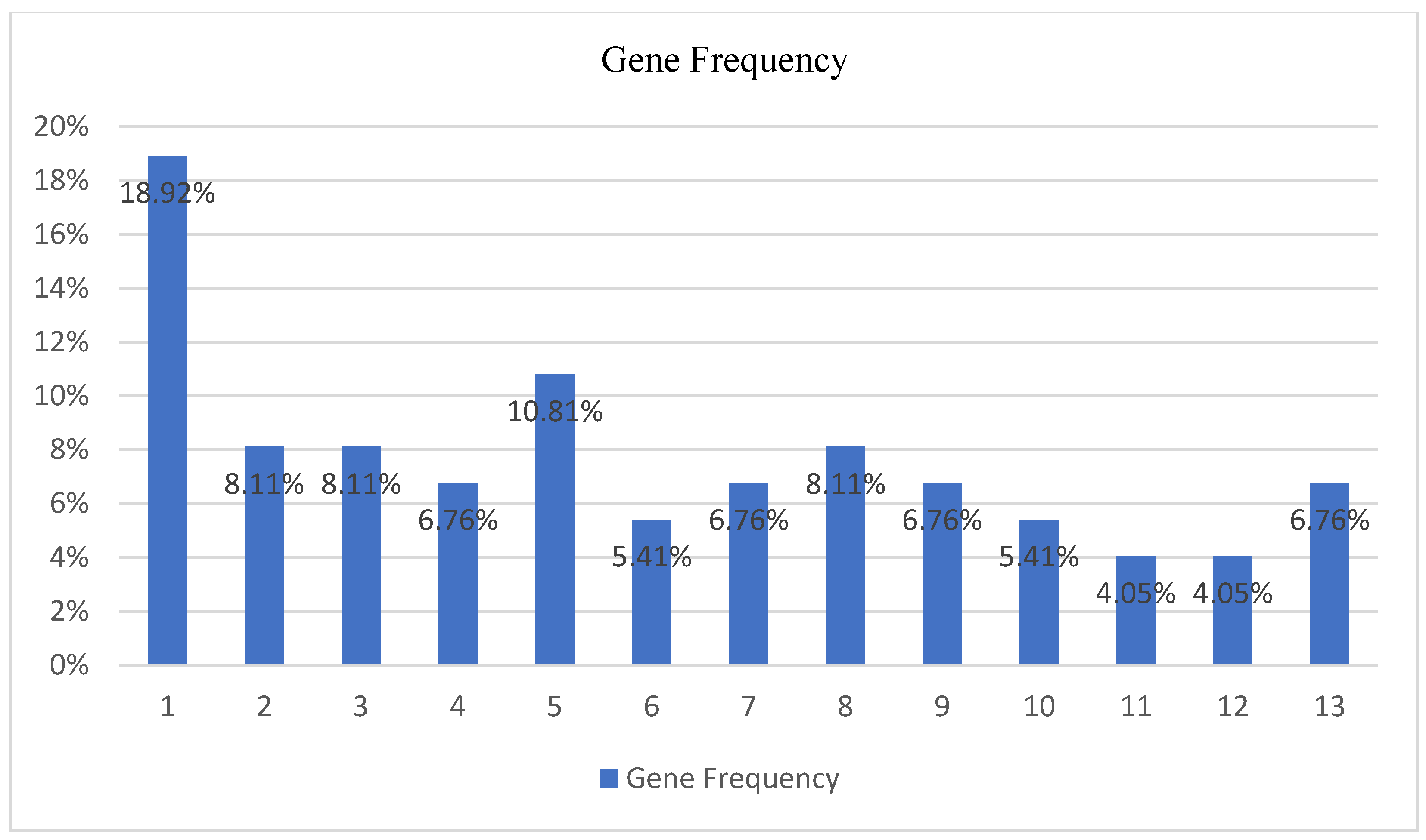
• First gene (v5—18.92%—When you When you find Greek products in the supermarkets do you prefer them over the imported products from abroad?);
• Second gene (v6—8.11%—During the health crisis (today) do you prefer Greek products more than before?);
• Third gene (v7—8.11%—Do you want the companies from which you choose to make some of your purchases to inform you in detail about the measures they have taken regarding coronavirus protection?);
• Fifth gene (v9—10.81%—After the health crisis, social life will be the same as before.);
• Eighth gene (v14—8.11%—During the health crisis the quantities we buy from the Super Markets have increased).

The average gene sequence includes almost half of the genes that are considered the best factors according to the outcome of the best chromosome gene occurrence for the class Household Size (see Figure 21, Table 12).

The genes that mostly participate in the classification procedure for class Household Monthly Income include:

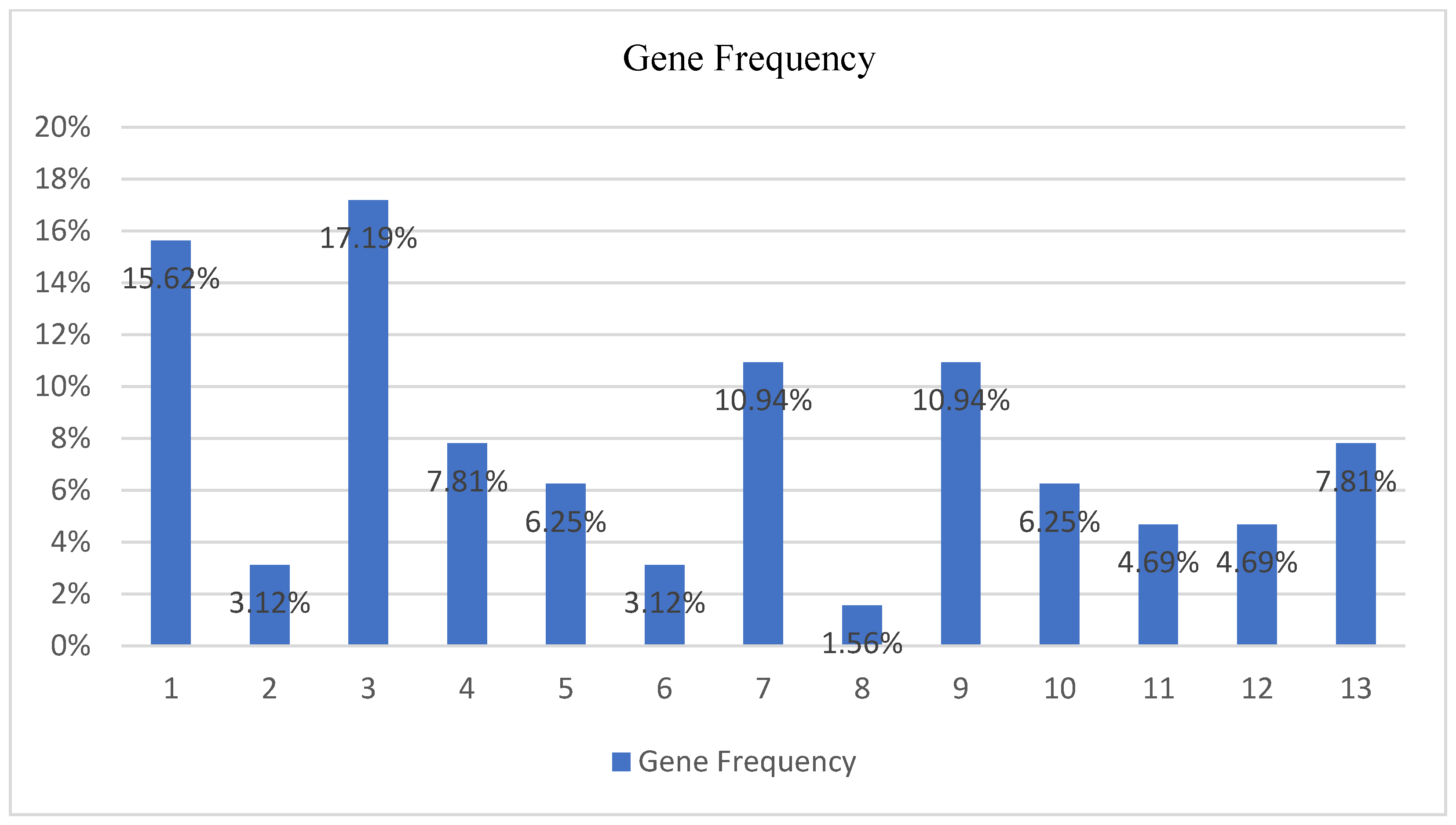
• First gene (v5—15.62%—When you When you find Greek products in the supermarkets do you prefer them over the imported products from abroad?);
• Third gene (v7—17.18%—Do you want the companies from which you choose to make some of your purchases to inform you in detail about the measures they have taken regarding coronavirus protection?);
• Fourth gene (v8—7.81%—After the health crisis, things will return to normal relatively quickly.);
• Seventh gene (v13—10.93%—The health crisis has affected the way we purchase.);
• Ninth gene (v15—10.93%—The health crisis has boosted online shopping.);
• Thirteenth gene (v22—7.81%—Approximately how much money do you spend every time you shop at the supermarkets now that we have a coronavirus problem (today)?).

The average gene sequence includes almost half of the genes that are considered the best factors according to the outcome of the best chromosome gene occurrence for the class Household Monthly Income (see Figure 22, Table 13).

These results verify the initial scope of this research. They also verify the results of the first phase of this method regarding the design methodology. Undoubtedly, these genes can be used to suggest new subsets of factors that can replace the primary set genes, and consent to the creation of new limited-in-size subsets that increase result accuracy, reduce the decision risk, and eliminate overfitting.

5.2.7. Rules Extraction

In conclusion, a set of rules extracted from the GA wrapper performance on consumer behaviour data provides promising findings which may have a significant impact to decision makers:

• The GA wrapper performs exceptionally well in small numeric datasets reaching classification accuracies above 90%;
• The current GA wrapper configuration, including the probability operators’ values, the number chromosomes, and the number of generations provide valid results;
• Referring to the Gender class and based on the average gene frequency of occurrence, a subset of four specific genes, including the first gene (v5—16.18%), the third gene (v7—10.29%), the seventh gene (v13—23.53%), and the tenth gene (v17—10.29%), can have a significant impact on defining the purchasing preferences based on gender differences;
• Referring to the Household Size class and based on the average gene frequency of occurrence, a subset of five specific genes, including the first gene (v5—18.92%), the second gene (v6—8.11%), the third gene (v7—8.11%), the fifth gene (v9—10.81%), and the eighth gene (v14—8.11%), can have a significant impact on defining the purchasing preferences based on the household size differences;
• Referring to the Household Monthly Income class and based on the average gene frequency of occurrence, a subset of six specific genes, including the first gene (v5—15.62%), the third gene (v7—17.18%), the fourth gene (v8—7.81%), the seventh gene (v13—10.93%), the ninth gene (v15—10.93%), and the thirteenth gene (v22—7.81%), can have a significant impact on defining the purchasing preferences based on the household monthly income impacts.

5.3. Research Contribution

This study manages to combine several concepts, methodologies, techniques, and data management theories and tools to provide a promising project that tries to narrow the gap between computers and marketing sciences and advance in the marketing research domain using new and applied artificial intelligence methods.

The basic scientific domains involved in this study include artificial intelligence, machine learning models, data mining techniques, marketing decision making, consumer behaviour, and applied statistics.

A part of this paper’s contribution is based on how the structure is stated, allowing potential researchers to conduct their own experiments and generate results following these steps. Despite the main goal of the paper, which is to create a novel machine learning model that can deliver optimised results for enhancing the decision-making process, it also generates new knowledge by examining collateral scientific fields. The main contributions include some new findings that inform the overall effort as follows:

• Combining the computer science theory and marketing science for better decision-making
• Providing examples of artificial intelligence applications on marketing data
• Conducting machine learning classification and optimisation methods performance evaluation
• Developing a machine learning method using classification and optimisation algorithms.
• Introducing a new way of generating subsets of features; instead of generating and classifying the optimal subsets of features as in previous research, this study calculates the features’ occurrence and their overall sequence of occurrence during the classification process. Thus, it provides a range of weighted features. Certain weights distinguish the best features, and decision-makers can determine the best final subsets.
• Keeping a track of the optimisation process by demonstrating the average and best fitness per generation
• Encapsulating the role of feature selection methods from past research works
• Introducing a variety of feature selection methods for optimal subset creation by calculating the features that mostly participated in the classification process and assigning certain weights of occurrence
• Producing subsets of features that affect consumers’ decisions
• Predicting consumer behaviour using marketing data insights
• Predicting consumer behaviour based on factors such as gender, household size, and household monthly income
• Providing a roadmap for conceiving, designing, developing, applying, and evaluating data optimisation through a data classification method [8]

The current study proposes a novel method to examine the factors that may affect consumer behaviour by using a machine learning method to combine data classification and feature selection techniques. A series of tests were conducted to prove the accuracy of the results. Feature selection statistical methods could have been used instead of this method. However, based on evidence from the literature [8], DTs and GAs can be combined to perform well.

Further applications of this method could be social media performance metrics analysis, where only the most effective metrics determine user behaviour, conversion rates, revenue, or total user engagement of a brand on a social media platform. Another application could refer to the search engine optimisation factors analysis, where this method could provide a subset of the initial factors that can help a website climb to the highest-ranking positions on search engine results pages. Regarding the generic marketing problems, this method could provide suggestions for consumer or user behaviour prediction, including features—gender, age, income, location, educational background, website speed, UX/UI of applications, average website visiting time, number of products, number of keywords, number of domain characters, etc.

5.4. Future Work

The study of machine learning methods and their comparison could be broadened by occasionally examining newly invented classification methods and applying them to the primary project or combining them with other optimisation methods, the applications of which would benefit decision-makers across sciences.

There are also some improvements that could complete the GA wrapper project and make it more robust. In order for these improvements to be effective, they should provide the option of multiple classification algorithm testing instead of a BDT. Moreover, the user can also have the option to examine and configure nominal, numeric, and multivariate variables through open access, user-friendly interface online, allowing them to make configurations and graphical representations.

Finally, regarding the consumer behaviour analysis, it is apparent that further investigation is needed to examine the adopted methodology and model with wider marketing–consumer behaviour data in order to validate its prediction power.

6. Conclusions

This research has shown how adaptive artificial intelligence can be in a consumer’s daily life. It is a powerful scientific area of computer science that can be potentially applied to every science. The GA wrapper managed to deliver valid results, indicating the complicated nature of data management, classification, and evaluation methods. The results are considered highly accurate, but their effectiveness is yet to be proven. Nonetheless, the study’s aim to provide data mining techniques for enhanced marketing decision-making using machine learning applications applied to the consumer’s behaviour and data gathered from online and offline environments is successful.

Regarding the consumer behaviour analysis, Gender, Household Size, and Household Monthly Income were associated with a specific set of variables providing a roadmap for the marketing decision-making. The GA wrapper performed exceptionally, reaching above 90% fitness. Referring to the Gender class, a subset of four genes, including the first, third, seventh, and tenth genes, can affect the consumers’ purchasing preferences based on their gender. Referring to the Household Size class, a subset of five genes, including the first, second, third, fifth, and eighth genes, can affect the consumers’ purchasing preferences based on their household size. Finally, referring to the Household Monthly Income class, a subset of six genes, including the first, third, fourth, seventh, ninth, and thirteenth genes, can affect the consumers’ purchasing preferences based on their household monthly income.

In future research or surveys focusing on the same subject, the marketing researcher is recommended to place emphasis on just this set of variables, i.e., a smaller set of questions to be addressed, a quicker analysis and results, and comparable conclusions.

Marketers can also analyse these associations and discover the core aspects that affect consumer behaviour. In our case, the preference for Greek products (country of origin of a brand) was found to be crucial for all three classes, indicating both the importance of the association and the determination degree of the variable. The same occurs when we examine the need of providing information from the firms regarding health subjects, the quantities of purchases from supermarkets, the money spent during a supermarket shopping visit, and the preference for physical or digital shopping [23]. All these variables determine the core attitudes of the consumers. Thus, marketing executives must focus on these aspects if they want their tactics to be consumer-oriented and competitive. At the same time, depending on the strategy adopted, decision-makers could target the consumer more effectively in terms of providing the appropriate bundle of these variables at a certain intensity relative to the profile of the household.

It is essential to pinpoint that this work, despite the interesting findings, has faced certain limitations that will hopefully be surpassed in the near future. Further research could try to broaden the number of platforms studied, industry sectors, data sources, and machine learning methods, and manage to distinguish any differences or discrepancies that may occur.

In conclusion, people are overwhelmed with the enormous amount of data in their daily lives; it seems there is no end in sight. While algorithms outperform human calculation capabilities, they can be used as a tool by humans. Artificial intelligence is now stronger than ever and ready to serve humanity, but the effort is still needed to reach a certain threshold to simulate human thinking. Nevertheless, it is expected that AI will eventually revolutionise the way information is managed. Brands, decision-makers, researchers, and consumers shape, willingly or not, will usher in the new AI landscape. Daily smartphone use, online data collection, research, and the desire for better solutions will rapidly evolve AI algorithms. Ethical AI aims to find solutions regarding privacy and surveillance concerns, biased data collection and discrimination, and, finally, the role of human judgment and freedom. Artificial intelligence ethics organisations, committees, and foundations have thus been shouldered with the monumental task of protecting citizens’ lives and privacy while building trust between brands and their consumers [24].

References

1. Beligiannis, G.; Skarlas, L.; Likothanassis, S. A Generic Applied Evolutionary Hybrid Technique. IEEE Signal Process. Mag. 2004, 21, 28–38. [Google Scholar] [CrossRef]
2. Sung, K.; Cho, S. GA SVM Wrapper Ensemble for Keystroke Dynamics Authentication. Adv. Biom. 2005, 3832, 654–660. [Google Scholar]
3. Yu, E.; Cho, S. Ensemble Based on GA Wrapper Feature Selection. Comput. Ind. Eng. 2006, 51, 111–116. [Google Scholar] [CrossRef]
4. Huang, J.; Cai, Y.; Xu, X. A Hybrid Genetic Algorithm for Feature Selection Wrapper Based on Mutual Information. Pattern Recognit. Lett. 2007, 28, 1825–1844. [Google Scholar] [CrossRef]
5. Rokach, L. Genetic Algorithm-based Feature Set Partitioning for Classification Problems. Pattern Recognit. 2008, 41, 1676–1700. [Google Scholar] [CrossRef] [Green Version]
6. Wang, D.; Zhang, Z.; Bai, R.; Mao, Y. A Hybrid System with Filter Approach and Multiple Population Genetic Algorithm for Feature Selection in Credit scoring. J. Comput. Appl. Math. 2018, 329, 307–321. [Google Scholar] [CrossRef]
7. Soufan, O.; Kleftogiannis, D.; Kalnis, P.; Bajic, V. DWFS: A Wrapper Feature Selection Tool Based on a Parallel Genetic Algorithm. PLoS ONE 2015, 10, e0117988. [Google Scholar] [CrossRef] [PubMed]
8. Rahmadani, S.; Dongoran, A.; Zarlis, M.; Zakarias. Comparison of Naive Bayes and Decision Tree on Feature Selection Using Genetic Algorithm for Classification Problem. J. Phys. Conf. Ser. 2018, 978, 012087. [Google Scholar] [CrossRef]
9. Hammami, M.; Bechikh, S.; Hung, C.; Ben Said, L. A Multi-objective Hybrid Filter-Wrapper Evolutionary Approach for Feature Selection. Memetic Comput. 2018, 11, 193–208. [Google Scholar] [CrossRef]
10. Dogadina, E.P.; Smirnov, M.V.; Osipov, A.V.; Suvorov, S.V. Evaluation of the Forms of Education of High School Students Using a Hybrid Model Based on Various Optimization Methods and a Neural Network. Informatics 2021, 8, 46. [Google Scholar] [CrossRef]
11. Chowdhury, A.; Rosenthal, J.; Waring, J.; Umeton, R. Applying Self-Supervised Learning to Medicine: Review of the State of the Art and Medical Implementations. Informatics 2021, 8, 59. [Google Scholar] [CrossRef]
12. Kohavi, R. Wrappers for Performance Enhancement and Oblivious Decision Graphs. Ph.D. Thesis, Stanford University, Stanford, CA, USA, 1996. [Google Scholar]
13. Mitchell, T.M. Machine Learning; McGraw-Hill: New York, NY, USA, 1997. [Google Scholar]
14. Russel, S.; Norvig, P. Artificial Intelligence: A Modern Approach, 3rd ed.; Prentice Hall: Hoboken, NJ, USA, 2003. [Google Scholar]
15. Witten, I.; Frank, E.; Hall, M. Data Mining; Morgan Kaufmann Publishers: Burlington, MA, USA, 2011. [Google Scholar]
16. Quinlan, J. Induction of Decision Trees. Mach. Learn. 1986, 1, 81–106. [Google Scholar] [CrossRef] [Green Version]
17. Quinlan, J. Simplifying Decision Trees. Int. J. Man-Mach. Stud. 1987, 27, 221–234. [Google Scholar] [CrossRef] [Green Version]
18. Blockeel, H.; De Raedt, L. Top-down Induction of First-order Logical Decision Trees. Artif. Intell. 1998, 101, 285–297. [Google Scholar] [CrossRef] [Green Version]
19. Mitchell, M. An Introduction to Genetic Algorithms; The MIT Press: Cambridge, MA, USA, 1996. [Google Scholar]
20. Whitley, D.A. Genetic Algorithm Tutorial. Stat. Comput. 1994, 4, 65–85. [Google Scholar] [CrossRef]
21. Hsu, W.H. Genetic Wrappers for Feature Selection in Decision Tree Induction and Variable Ordering in Bayesian Network Structure learning. Inf. Sci. 2004, 163, 103–122. [Google Scholar] [CrossRef]
22. Davis, L. Handbook of Genetic Algorithms; Van Nostrand Reinhold: New York, NY, USA, 1991; p. 115. [Google Scholar]
23. Theodoridis, P.K.; Kavoura, A. The Impact of COVID-19 on Consumer Behaviour: The Case of Greece. In Strategic Innovative Marketing and Tourism in the COVID-19 Era, Springer Proceedings in Business and Economics; Kavoura, A., Havlovic, S.J., Totskaya, N., Eds.; Springer: Ionian Islands, Greece, 2021; pp. 11–18. [Google Scholar] [CrossRef]
24. Data Ethics. Available online: https://dataethics.eu/danish-companies-behind-seal-for-digital-responsibility (accessed on 15 August 2020).
Figure 1. Genetic Algorithm Wrapper Model. This figure demonstrates the overall wrapping classification and data exchange procedure of the binary decision tree and the genetic algorithm.
Informatics 09 00045 g001
Figure 2. Genetic Algorithm Wrapper Flowchart. The flowchart shows the information transition during the classification and optimization processes.
Informatics 09 00045 g002
Figure 3. GA Wrapper Procedures Abstract Dataflow Diagram. This figure includes all the information required to make the reader comprehend the nature of generations, the role of operators, and the split criteria.
Informatics 09 00045 g003
Figure 4. Optimal Feature/Chromosome Representation. This is the main chromosome representation, along with including the gene positions, which are indicated with black colour, while the classes genes are indicated with red colour. * times symbol.
Informatics 09 00045 g004
Figure 5. Dominant Training BDT for Gender Classification.
Informatics 09 00045 g005
Figure 6. Dominant Validation BDT for Gender Classification.
Informatics 09 00045 g006
Figure 7. Dominant Testing BDT for Gender Classification.
Informatics 09 00045 g007
Figure 8. Dominant Training BDT for Household Size Classification. * times symbol.
Informatics 09 00045 g008
Figure 9. Dominant Validation BDT for Household Size Classification. * times symbol.
Informatics 09 00045 g009
Figure 10. Dominant Testing BDT for Household Size Classification. * times symbol.
Informatics 09 00045 g010
Figure 11. Dominant Training BDT for Household Monthly Income Classification. * times symbol.
Informatics 09 00045 g011
Figure 12. Dominant Validation BDT for Household Monthly Income Classification. * times symbol.
Informatics 09 00045 g012
Figure 13. Dominant Testing BDT for Household Monthly Income Classification. * times symbol.
Informatics 09 00045 g013
Figure 14. Best Chromosome Testing BDT for Gender. Bold highlights the best selected chromosomes.
Informatics 09 00045 g014
Figure 15. Dominant Testing BDT for Household Size Classification. Bold highlights the best selected chromosomes. * times symbol.
Informatics 09 00045 g015
Figure 16. Dominant Testing BDT for Household Monthly Income Classification. Bold highlights the best selected chromosomes. * times symbol.
Informatics 09 00045 g016
Figure 17. GA Wrapper Performance on Gender Data.
Informatics 09 00045 g017
Figure 18. GA Wrapper Performance on Household Size Data.
Informatics 09 00045 g018
Figure 19. GA Wrapper Performance on Household Monthly Income Data.
Informatics 09 00045 g019
Figure 20. GA Wrapper Performance on Household Size Data.
Informatics 09 00045 g020
Figure 21. GA Wrapper Performance on Household Size Data.
Informatics 09 00045 g021
Figure 22. GA Wrapper Performance on Household Monthly Income Data.
Informatics 09 00045 g022