Fraction Factorial Design of a Novel Semi-Transparent Layer for Applications on Solar Roads

Abstract

Solar roads are transportation infrastructures able both to generate electricity thanks to solar cells placed under a semi-transparent layer and to ensure heavy traffic circulation. In this paper, a novel transparent top layer made of glass aggregates bonded together using a polyurethane glue is presented. The goal is to design a composite material able to support traffic load, guarantee vehicle skid-resistance, allow the passage of sunlight, and protect the solar cells. For this purpose, the authors investigated the effect of different variables (thickness, glue content, and glass aggregate distribution) on the mechanical and optical performances of the material applying the factorial design method. The semi-transparent layer was characterized by performing the three-point bending test and measuring the power loss. Regarding the vehicle friction, experimental tests with the British Pendulum were conducted in order to measure the skid resistance of the surface and compare it with the specifications of a typical road infrastructure. According to the fraction factorial design and the British Pendulum test, the following mixture was developed: 42.8% of 4/6 mm; 42.8% of 2/4 mm, 14.4% of glue in volume, and a thickness of 0.6 cm. The first results are encouraging, and they demonstrate the feasibility of a semi-transparent layer for future applications in full scale.

1. Introduction

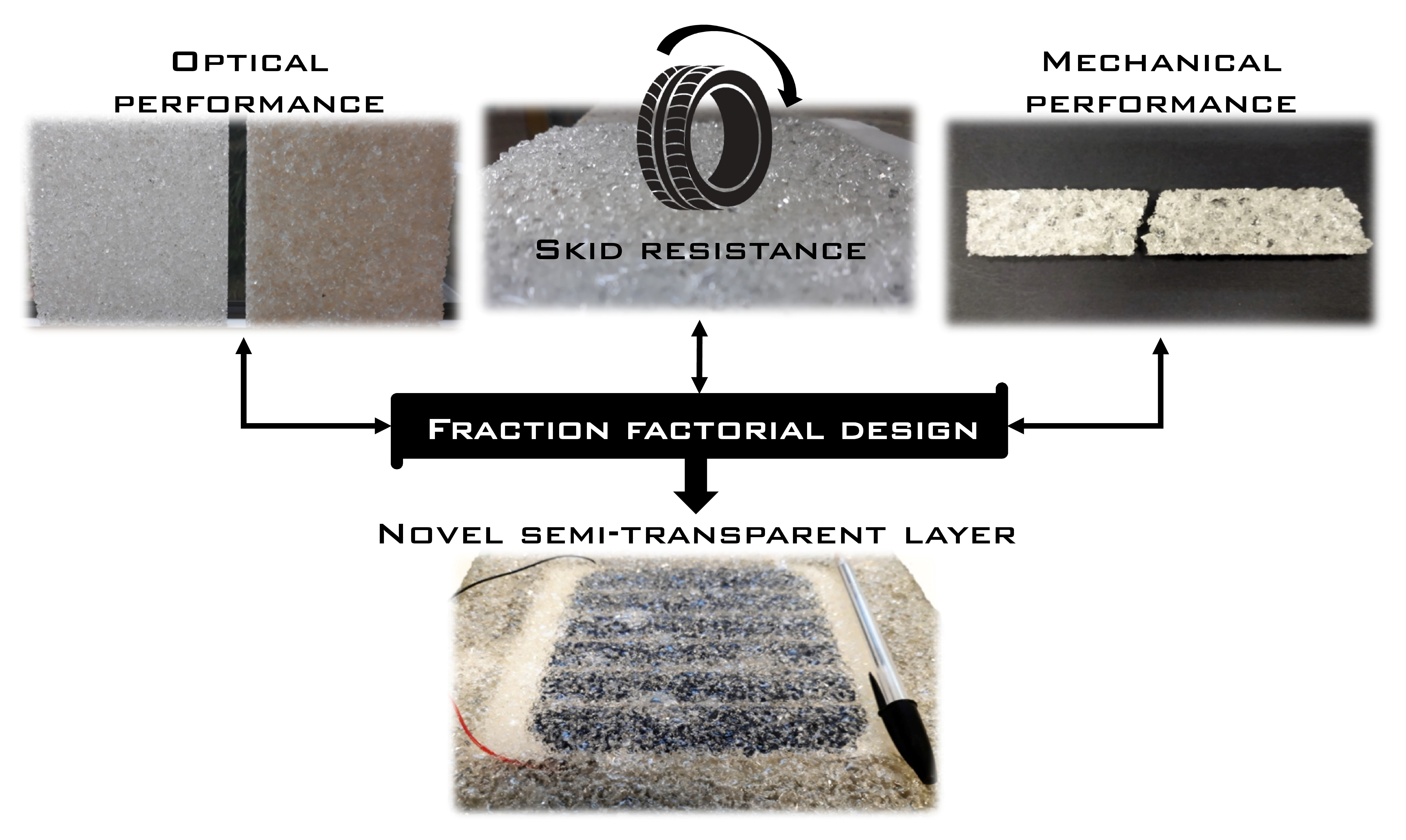
A photovoltaic road is a pavement system able to convert the sunlight in electricity thanks to the photovoltaic effect. A typical photovoltaic road is composed of three layers [1,2,3]: the top element is a transparent surface of tempered glass or a mixture made of glass aggregates bonded together using a transparent resin (i.e., epoxy, polyurethane, etc.); the second layer contains the solar cells and the base layer, which has to transmit the traffic load to the pavement, subgrade or base structure (Figure 1) [4].

In terms of energy, the electrical output of a photovoltaic road depends on the amount of solar radiations that hits the pavement during the year and on the efficiency of the solar cells. Unfortunately, the electrical output is also affected by the low transparency of the top layer and the presence of dust.

One of the first prototypes of the photovoltaic road was launched by Solaroadway in 2009. The system, able to generate an electrical power of 88–108 W/m², is a hexagonal panel composed of several solar cells enclosed between two layers of tempered glass hermetically sealed. Furthermore, several light-emitting diode (LED) lights are imbedded into the pavement to make road lines and signage [5].

In the Netherlands in 2014, a consortium of research institutions and industries installed a photovoltaic cycle path. The road is 70 m in length and 3.5 m in width and was developed as prefabricated slabs. Each slab is a concrete module of 2.5 by 3.5 m, covered by a top layer of tempered glass having a thickness of 1 cm [6].

In 2016 in France, the Colas Company built 1 km of solar pavement, having an electrical output of 280 MWh/year. The technology consists of panels containing 15-cm wide polycrystalline silicon cells that transform the solar energy into electricity. The cells are coated in a multilayer substrate composed of resins and polymers, translucent enough to allow sunlight to pass through, and resistant enough to withstand truck traffic [7].

In 2018 in China, the Qilu Transportation Development Group built the longest photovoltaic road, able to generate 1 million KWh per year. The infrastructure has a length of 1 km and covers an area of 5875 m² over two lanes and one emergency lane [8].

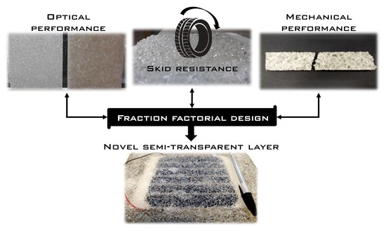
All these pavements have in common the top surface made of tempered glass or resins. The idea of the authors is to design a novel semi-transparent layer, made of glass aggregates bonded together through a transparent polyurethane.

Besides the materials, another difference is the ease of manufacturing procedure. This is carried out by mixing together glass aggregates and binder and laying down the material in a specific mold.

2. Materials and Methodology

The paper begins with a brief characterization of the polyurethanes, paying attention to the influence of the temperature in terms of curing time and strength.

Second, the semi-transparent layer is designed thanks to factorial design. This method describes, through a multiple regression model, the influence of each mix variable (thickness, glue content, and glass aggregate distribution) on the optical and mechanical performances of the material.

Finally, the semi-transparent layer is evaluated in terms of friction by performing the British Pendulum and the results are compared with standards for typical roads.

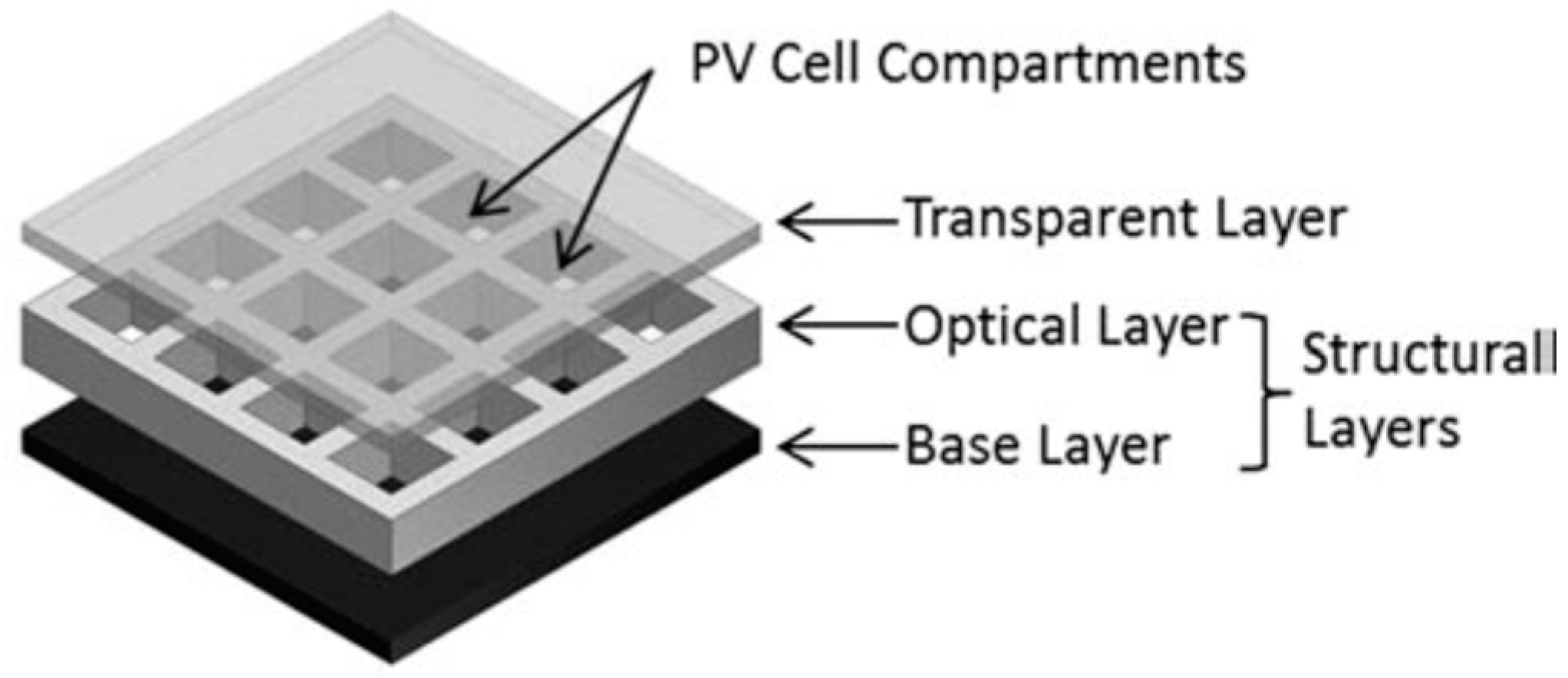
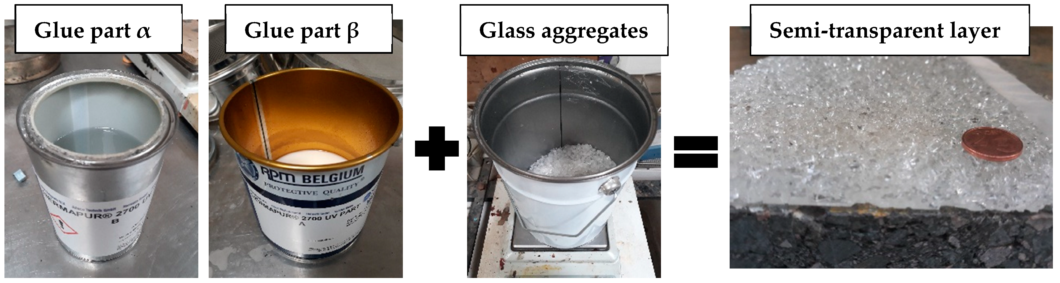
In terms of materials, the semi-transparent layer is composed of recycled glass aggregates bonded together using a polyurethane glue.

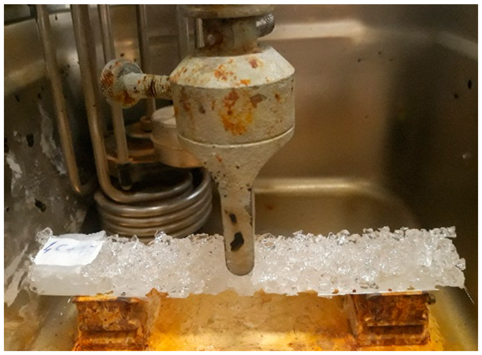
The procedure for preparing samples consists of a manual mix of the glass aggregates with the polyurethane for three minutes. The result is a uniform mixture with a good workability that must be quickly laid on the mold before the beginning of the polymerization (Figure 2). The compaction is very low, and it is carried out manually.

The choice of polyurethane (instead of epoxy) is due to its good transparency, good adhesion on glass and its resistance to sunlight exposition. In fact, previous experiments show that the epoxy becomes brittle and yellow in a short time [9].

The glass aggregates were separated according to three fractions: 4/6 mm, 2/4 mm, and 0.064/2 mm. In this analysis, the filler (aggregates <0.064 mm) was removed because it could have a negative impact on the transparency of the surface.

Four different types of polyurethane (A, B, C, and D) were tested. Each polyurethane was obtained by mixing together two components: the diisocyanate, called component α (containing two or more –NCO groups) and the polyfunctional hydroxy compounds, called component β (containing the –OH group) [10]. The properties of the polyurethanes and the proportions of each component are listed in

Table 1. Properties of the polyurethanes.

Ref.	Part	Boiling Point (°C)	Flash Point (°C)	Viscosity (mPa s)	Density (gr/cm3)	Mass Fraction (%)
A	α	170	220	3000 (20 °C)	1	50
	β	NA	158	1200 (20 °C)	1.2	50
B	α	170	200	700 (20 °C)	1	47.5
	β	285	203	1000 (20 °C)	1.15	52.5
C	α	200	70	600 (20 °C)	1.3	58.7
	β	200	200	1000 (20 °C)	1.13	41.3
D	α	200	70	700 (20 °C)	1.1	57.8
	β	231	183	596 (20 °C)	1.15	42.2

[11].

Compared with a typical bitumen, the polyurethane behaves like a thermosetting material, in other words it becomes chemically crosslinked during final molding or curing [12].

The mix of the components α and β triggers the polymerization and the process is strongly dependent on the temperature. For example, at 50 °C and 10 °C the curing time is respectively 2–3 h and 40–50 h. Because of the strong dependency of the curing time on the temperature, the experimental data were modelled using the Arrhenius law.

The general equation of the Arrhenius law is given by:

$$k=\mathsf{\Delta }{e}^{-E/RT}$$

(1)

where k is the rate constant (s⁻¹) for a reaction of the first order; E is the activation energy (J/mol), R is the universal gas constant (8.314 J/K*mol); Δ is a pre-exponential factor (s⁻¹); T is the temperature (K). In particular, the parameters E and Δ regulate the speed of the reaction and their values are listed in

Table 2. Values of pre-exponential factor Δ and activation energy E for the polyurethanes.

Polyurethane	(1/s)	E (J/mol)
A	4.83 × 109	80,445
B	1.42 × 106	61,566
C	5.75 × 105	59,274
D	6.30 × 103	49,126

[11].

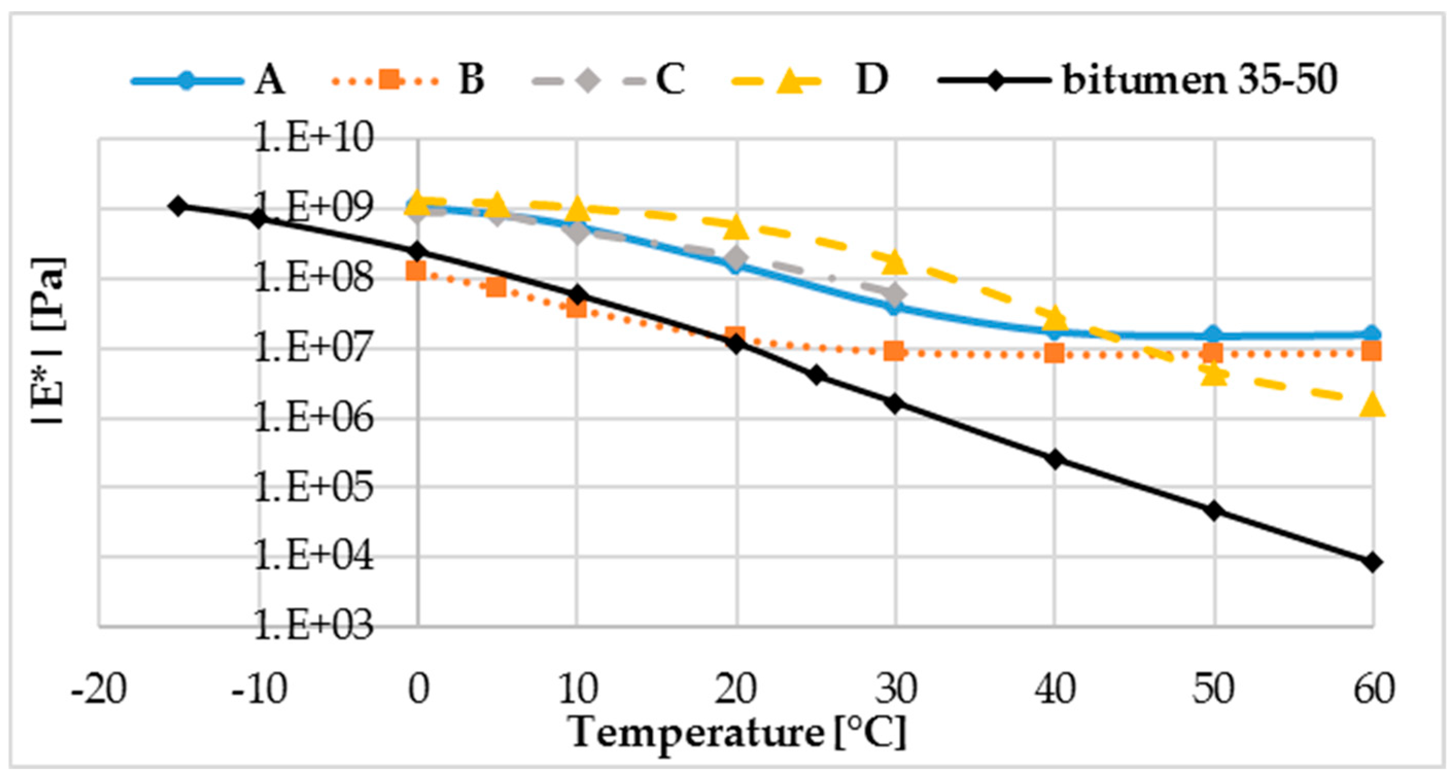
Once the curing time was satisfactorily determined, the dynamic mechanical analysis was performed on the solid samples, cured at 20 °C for a curing time of around 24 h. The test provided the complex modulus E* of each polyurethane in tension-compression for various frequencies and temperatures. The complex modulus (E*) is defined as the relationship between the complex strain and the complex stress and it is given by the sum of two components: the elastic modulus, which represents the ability of the material to store energy and the viscous modulus, which represents the ability of the material to dissipate energy.

The test was performed in a range temperature of 0–60 °C for the frequency of 1 Hz, which guarantees acceptable results both in the glassy and rubbery state (Figure 3).

The figure shows the glues behave like thermosetting polymers. At low temperatures (<0 °C), it is reasonable to assume that the polyurethanes are in the glassy region, characterized by a complex modulus higher than 10⁹ Pa [13]. As the temperature increases (>0 °C), the modulus falls through the glass transition region where the glues behave like a viscoelastic material and the complex modulus is temperature dependent. At higher temperatures, the polyurethanes are in the rubbery plateau region and the complex modulus stabilizes [14]. In more detail, for the glue A, B, and C, the rubbery plateau region starts at 40 °C and the complex modulus is around 1 × 10⁷ Pa, while the glue D is still in the glass transition region. In comparison with a typical bitumen 35–50, the polyurethanes A, C, and D are stiffer, especially for temperatures higher than 20 °C.

The glue B is similar independent of the temperature (complex moduli of 10⁸ to 10⁷ Pa). For the conventional asphalt binder, it changes a lot (complex moduli of 10⁸ to 10⁴ Pa). In the perspective of an application in situ, this result is encouraging, considering that a solar road could be built in hot areas, having very high temperatures during the summertime.

3. Factorial Design

The optimization of the semi-transparent layer was performed using the factorial design, a method able to study the influence of each experimental variable and their interaction on the response of the investigated system.

In the field of road engineering, the factorial design method has been applied on many occasions for example to investigate the resilient modulus of bituminous paving mixes [15], or to analyze the effect of recycled coarse aggregates percentage and bitumen content percentage on various parameters such as stability, flow, air void, void mineral aggregate, void filled with bitumen, and bulk density [16]. Wang et al studied the effects of basalt fiber content, length, and asphalt-aggregate ratio on the volumetric and strength properties of styrene–butadiene–styrene (SBS)-modified asphalt mixture [17]. A two-level factorial design was developed to evaluate the effects of the test temperature and of a surfactant warm additive on the visco-elastic behavior of a bitumen [18]. Kabagire et Yahia applied the full-factorial design on pervious concrete, in order to study the effect of three mixture parameters (paste volume- to-inter-particles void ratio, water-to-cement ratio, and dosage of water reducing agent) on permeability, effective porosity, unit weight, and compressive strength [19].

Zou et al evaluated the effect of asphalt mixture type, temperature, loading frequency and tire- pavement contact pressure on the wheel tracking test [20].

Based on the literature, the factorial design seems to be a good method to better-understand the effects of a high number of variables on the outcome of the investigated system, especially when the system to be modeled is complex.

In this case, the factorial design was applied to evaluate the influence of thickness, glass fractions, and glue content on both the mechanical and optical performance of the semi-transparent layer.

3.1. Mix-Design Based on the Fraction Factorial Design

The factorial design is a multipurpose tool that can be used in various situations for identification of important input factors (input variable) and how they are related to the outputs [21]. If the influence of a certain number of h variables is investigated, the factorial design will consist of 2^h experiments.

Each experiment provides a system’s response, according to the variable combinations. The goal is to describe the response of the system fitting a multiple regression model given by:

$$y=a_0+\sum a_i{x}_i+\sum a_{ij}{x}_i{x}_j+\dots +\sum a_{ii}{x}_i^2+a_{ij\dots z}{x}_i{x}_j\dots x_z+e$$

(2)

Considering only the second order interactions, (2) becomes:

$$y=a_0+\sum a_i{x}_i+\sum a_{ij}{x}_i{x}_j+e$$

(3)

The factorial design can be defined as a system of n equations (each equation is given by an experiment) and p variables [22], which can be written in matrix format as:

$$\overline{y}=\stackrel{=}{X}\overline{a}+\overline{e}$$

(4)

where:

• $\overline{y}$ is the vector with the outcome of the experiments;
• $\stackrel{=}{X}$ is the model matrix, depending on the interactions between the variables;
• $\overline{a}$ is the vector with the coefficient of the regression model;
• $\overline{e}$ is the error.

In most investigations it is reasonable to assume the influence of the third order or higher is negligible. It means that it is possible to reduce the number of experiments, changing from 2^h to 2^h-p experiments. This method is called fraction factorial design, where p is the size of the fraction.

On reducing the number of experiments and consequently of the equations, the system (3) is no longer solvable (n number of equations <p unknown coefficients). The idea is to cofound some effects, defining some equivalences between the variables and consequently reduce the unknown coefficients [23].

The fraction factorial design was applied to study the effect of five variables on the optical and mechanical performances of the semi-transparent layer and for each variable an experimental domain was defined (

Table 3. Experimental domain of the variables.

Variables	(−1) Level	(+1) Level
x1 = glass fraction 4/6 mm (%)	20	60
x2 = glass fraction 2/4 mm (%)	20	60
x3 = glass fraction 0/2 mm (%)	0	50
x4 = glue content (%)	5	20
x5 = thickness (cm)	0.6	1

).

The level −1 and +1 represent the minimum and maximum values of each variable and they are the boundary of the domains.

If the full factorial design was applied, the number of experiments would be equal to 2⁵ = 32. This is very time-consuming and for this reason the ¼ factorial design was introduced. In other terms, the number of experiments was reduced to 2⁽⁵⁻²⁾ = 8, cofounding the last two variables as:

• x4 = x1 × x2
• x5 = x1 × x2 × x3

Based on the previous assumptions, the model matrix $\stackrel{=}{X}$ is given by

Table 4. Model matrix.

	I	x1	x2	x3	x1 × x2 = x4	x1 × x3	x2 × x3	x1 × x2 × x3 = x5
Exp1	+1	−1	−1	−1	+1	+1	+1	−1
Exp2	+1	+1	−1	−1	−1	−1	+1	+1
Exp3	+1	−1	+1	−1	−1	+1	−1	+1
Exp4	+1	+1	+1	−1	+1	−1	−1	−1
Exp5	+1	−1	−1	+1	+1	−1	−1	+1
Exp6	+1	+1	−1	+1	−1	+1	−1	−1
Exp7	+1	−1	+1	+1	−1	−1	+1	−1
Exp8	+1	+1	+1	+1	+1	+1	+1	+1

.

+1 and −1 represent the extreme values of each variable (defined in the Table 3), while the column I, containing only +1, is used to compute the average response of the system and it is necessary to obtain a square matrix [24].

Replacing the terms of the model matrix (Table 4) with the extreme values of each variable, the following experiments were derived (

Table 5. Mix-design of each experiment.

Experiment n.	x1 = 4/6 mm (%)	x2 = 2/4 mm (%)	x3 = 0/2 mm (%)	x4 = glue (%)	x5 = thickness (cm)
1	33.3	33.3	0	33.3	0.6
2	70.6	23.5	0	5.9	1
3	23.5	70.6	0	5.9	1
4	42.8	42.8	0	14.4	0.6
5	18.2	18.2	45.4	18.2	1
6	44	15	37	4	0.6
7	15	44	37	4	0.6
8	31.6	31.6	26.3	10.5	1

):

3.2. Optical Performance

Once the mixes design was defined based on the fraction factorial design (Table 5), the influence of thickness, glue content and glass aggregates distribution on the optical performance of the semi- transparent layer was evaluated. The test was performed twice for each experiment and the average was calculated. The test was carried out on samples having dimensions of 160 × 160 × 10 mm³ or 160 × 160 × 6 mm³.

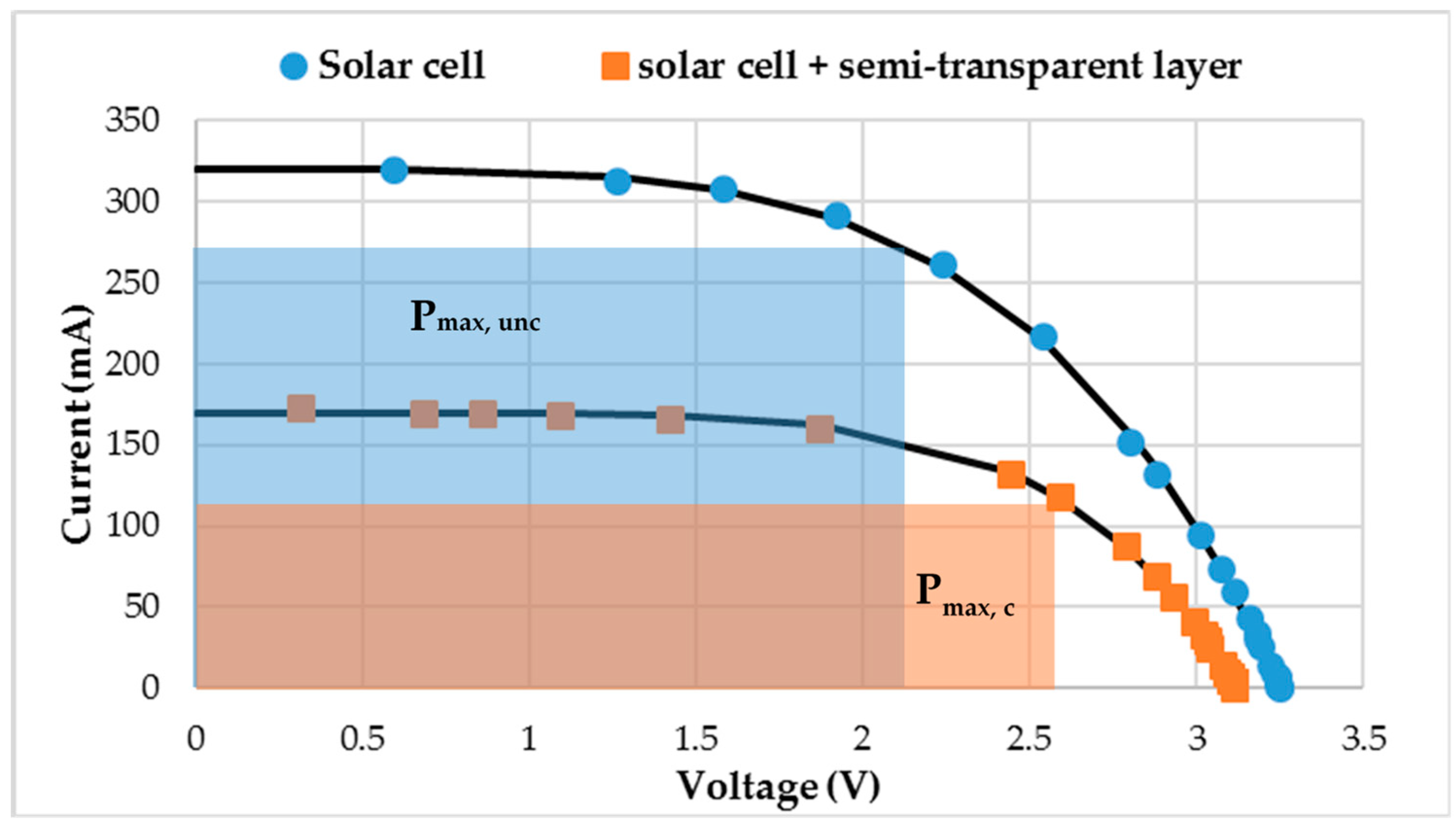
The optical performance was calculated in terms of power loss of the solar cell because of the semi-transparent layer. The scope of this test is to generate the sunlight radiation in a controlled environment and to measure the power reduction. The equipment is composed of: (i) a halogen lamp of 400 W placed in a box; (ii) a solar cell having dimensions 15 cm × 15 cm with a peak power of 15 W, an open circuit voltage Voc of 19.5 V and a short circuit current Isc of 0.97 A in standard conditions (Irradiance of 1000 W/m² and temperature of 25 °C); (iii) a solarimeter to check the stability of the radiation during the test; (iv) a set of resistances between 2 and 5000 Ω; (v) two multimeters to measure simultaneously the intensity current and the voltage of the solar cell for each resistance, and (vi) a thermometer to control the temperature in the box. The test provides the intensity-voltage curve of the solar cell (Figure 4) and its maximum power point.

The test is then repeated covering the solar cell with the semi-transparent layer and measuring again the intensity-voltage curve and the maximum power point. Finally, the power loss (PL) can be calculated according to the formula:

$$PL=\frac{\left(P_{max,unc}-P_{max,c}\right)}{P_{max,unc}}100$$

(5)

where: P_max,unc is the maximum power point of the solar cell and P_max,c is the maximum power point of the solar cell covered by the semi-transparent layer.

The PL ranges theoretically between 0% (top layer perfectly transparent) and 100% (top layer totally black).

The test was performed for each mix of Table 5 and the values of power loss are the elements which form the vector $\overline{y}$ (Equation (3)).

Based on the results of the

Table 6. Vector $\overline{y}$ containing the value of power loss measured for each mix.

Experiment n.	Power Loss (%)
1	44.8
2	69.0
3	65.0
4	43.1
5	69.7
6	74.2
7	76.4
8	73.1

, the vector $\overline{a}$ (Equation (3)) can be derived and the regression model describing the optical performance of the semi-transparent layer is given by:

$$\begin{array}{l}y=64.41+0.437x_1-0.012x_2+8.937x_3-6.737x_4-0.141x_1{x}_2+1.412x_2{x}_3\\ +4.787x_5\end{array}$$

(6)

The minimum of the regression model, into the domain variables of Table 3, is 42.2% and it represents the minimum of achievable power loss for the semi-transparent layer.

The solution is given for the following mix-design (

Table 7. Mix-design to minimize the power loss of the semi-transparent layer.

Variable		Value	Mix-Design
x1	Glass 4/6 mm	−1	20%
x2	Glass 2/4 mm	1	60%
x3	Glass 0/2 mm	−1	0%
x4	% glue	1	20%
x5	Thickness	−1	0.6 cm

).

According to Equation (6), the influence of each variable on the power loss is reported in Figure 5.

The glass fraction 0.064/2 mm has a negative impact on the power loss of the semi-transparent layer. In fact, the small dimensions of the aggregates interfere with the sunlight wavelengths, reducing the radiation intercepted by the solar cells [25,26].

When the glue content is 0%, the solar radiation strikes only the granular surface of the glass aggregates and, because of its irregularity, the light bounces off in all directions. This phenomenon is called diffuse reflection [27]. On increasing the glue content, the surface of the semi-transparent layer tends to be more regular, the diffuse reflection is reduced and more radiation can reach the solar cell.

As expected, the increase of the thickness reduces the power loss. According the Beer–Lambert law, for a given medium, the light attenuation is exponential with the path length through which the light is travelling [28].

Summarizing, considering the optical performance, the results show a negative impact for fine particles and thickness and a positive impact for glue content. Furthermore, the power loss is more sensitive to the fine particles than the thickness.

3.3. Mechanical Performance

The influence of each variable on the mechanical performance was studied following the same approach described for the optical performance. The mixtures were compared performing the three- point bending test (Figure 6), which measures the deflection-force curve of the material until rupture. The test was performed twice for each experiment and the average was calculated. The test was carried out at 20 °C, on rectangular samples having dimensions 90 × 25 × 10 mm³ or 90 × 25 × 6 mm³ and calculating the maximum stress in the mid-section [29].

Assuming that (i) the specimen of glass and glue is a beam composed of a homogeneous and elastic material and (ii) the beam is supported at two points and loaded in the midpoint, the stress– strain curve was derived according to Equations (7) and (8):

$$\mathsf{\sigma }=\frac{3\mathrm{PL}}{2{\mathrm{bh}}^2}$$

(7)

$$\mathsf{\epsilon }=\frac{6\mathsf{\delta }\mathrm{h}}{{\mathrm{L}}^2}$$

(8)

where: σ and ε are the stress and the strain calculated in the central vertical section of the beam; F is the load applied by the device; b and h are the dimensions of the sample’s section; δ is the deflection in the midpoint measured during the test; L is the span beam.

During the test, the fibers of the lower face undergo a tension state. Considering the central vertical section, the maximum positive stress σ_max is to the bottom surface.

The area of the stress–strain curve until rupture is the toughness t, which represents the energy that the material can absorb before the rupture.

The toughness was chosen as the outcome in the fraction factorial design to describe the mechanical performance of the material. Based on the results of the three-point bending test on the mixtures listed in Table 5, the vector $\overline{y}$ was derived (

Table 8. Vector $\overline{y}$ containing the value of toughness measured for each mix.

Experiment n.	Toughness (MPa)
1	0.1620
2	0.0010
3	0.0017
4	0.0184
5	0.1400
6	0.0006
7	0.0005
8	0.6240

).

The regression model, which describes the influence of each variable on the toughness of the material, is given by Equation (9):

$$\begin{array}{l}y=0.048-0.0278x_1-0.0276x_2+0.003x_3+0.0474x_4+0.0083x_1{x}_2+0.0081x_2{x}_3\\ +0.0029x_5\end{array}$$

(9)

The maximum of Equation (9) is 0.168 MPa and it is the maximum of achievable toughness in the variables domain of Table 3. The solution is given for the following mix design (

Table 9. Mix-design to maximize the toughness of the semi-transparent layer.

Variable		Value	Mix-Design
x1	Glass 4/6 mm	−1	37.5%
x2	Glass 2/4 mm	−1	37.5%
x3	Glass 0/2 mm	−1	0%
x4	% glue	1	25%
x5	Thickness	1	1 cm

).

According to Equation (9), the influence of each variable on the toughness is reported in Figure 7.

The glue content has a positive impact on the toughness of the semi-transparent layer, as observed for the optical performance.

The toughness can be also improved by mixing two glass fractions (i.e., 2/4 mm and 4/6 mm). In fact, the mix of two fractions optimizes the packing density, reducing the air voids and improving the strength of the material.

Summarizing, considering the mechanical performance (toughness), the results show negative impact for large and intermediate size particles and positive impact for glue content.

4. Skid Resistance

The skid resistance of the semi-transparent layer was evaluated using the British Pendulum [30,31]. The test was performed for the mixtures of Table 5 and the results are listed in

Table 10. Values of BPN for the mixtures of Table 5.

Experiment n.	BPN (British Pendulum Number)
1	46
2	67
3	69
4	65
5	53
6	86
7	89
8	75

.

The results of BPN (British Pendulum Number) range between 46 and 89. The lowest value of BPN corresponds to the mix design of experiment 1, having the highest glue content (33.3%) and lowest aggregates in volume. In this condition, the surface appears smoother and not very homogenous. Considering that the aggregates provide the skid resistance, the low value of BPN is consistent with the mix-design of experiment 1. On the other hand, the mix designs of the experiments 6 and 7 have a BPN of 86 and 89, respectively. In this case, the glue content is only 4% and the surface is rougher and without smooth parts.

All other mixtures have a BPN higher than 65, which fulfills the requirements of skid resistance “even of fast traffic and thus making it most unlikely that the road will be the scene of repeated accidents” [32].

5. The Optimal Mixture

Taking into account the results of both optical and mechanical performances, the optimal mixture will have high glue content, absence of fine particles, and low thickness.

Anyway, the glue content must not exceed 20% in volume, because it will reduce the skid resistance. The high glue content also causes a reduction of workability of the material. In fact, the glue tends to settle on the bottom of the mold and the result is a non-homogeneous mixture.

Based on these observations, the authors proposed the following solution (

Table 11. Optimal mix-design for both mechanical and optical performances.

Variable		Mix-Design
x1	Glass 4/6 mm	42.8%
x2	Glass 2/4 mm	42.8%
x3	Glass 0/2 mm	0%
x4	% glue	14.4%
x5	Thickness	0.6 cm

), corresponding to experiment number 4 of Table 5.

6. Conclusions

In this paper, a novel semi-transparent layer made of glass aggregates and polyurethane was designed for application in solar roads. Once the materials were characterized, the authors studied the influence of each variable (thickness, glass fraction, and glue content) on the optical and mechanical performance of the semi-transparent layer, applying the fraction factorial design method. The outcomes were two regression models describing the behavior of the material in terms of power loss of the solar cell and toughness.

The model of Equation (9) shows that the mechanical performance can be maximize by increasing the glue content. This result is coherent with the manufacturing procedure of the semi-transparent layer. It consists of very low compaction, which does not provide any additional strength to the material. The strength is provided by the glue and by a proper design of the grading curve.

The toughness can be slightly improved by using the glass fraction 0.064/2 mm. On the other hand, the fine particles interfere with the wavelength of the sunlight, reducing dramatically the radiation intercepted by the solar cells.

For this reason, a compromise was required and the authors proposed a mixture of 0.6 cm of thickness, having the following content: 42.8% of 4/6 mm; 42.8% of 2/4 mm and 14.4% of glue in volume.

In terms of skid resistance, the semi-transparent layer meets the standard. A problem may arise for high glue content (˃20%). In this case, the surface could be not uniform, with some lack of aggregates and the presence of glue on the surface. This could cause loss of friction and trigger hydroplaning. Another problem could be the presence of dirt or dust, which reduces the transparency of the surface. The solution is routine cleaning of the top layer.

Further research will focus on a better comprehension of the chemical reactions that trigger the aging process and their effects on the optical and mechanical performance of the semi-transparent layer.