On the Representativeness of the Cohesive Zone Model in the Simulation of the Delamination Problem


1
Faculty of Engineering, The University of Nottingham, Nottingham NG8 1BB, UK
2
Beijing Institute of Aeronautical Materials, Wenquan, Haidian District, Beijing 100095, China
*
Author to whom correspondence should be addressed.
J. Compos. Sci. 2019, 3(1), 22; https://0-doi-org.brum.beds.ac.uk/10.3390/jcs3010022
Submission received: 24 January 2019
/
Revised: 17 February 2019
/
Accepted: 22 February 2019
/
Published: 28 February 2019
Abstract
:With the development of finite element (FE) codes, numerical modelling of delamination is often considered to be somewhat commonplace in modern engineering. However, the readily available modelling techniques often undermine the truthful understanding of the nature of the problem. In particular, a critical review of the representativeness of the numerical model is often diverted to merely a matter of numerical accuracy. The objective of this paper is to scrutinise the representativeness of cohesive zone modelling (CZM), which is readily available in most of the modern FE codes and is used extensively. By concentrating on obtaining the converged solution for the most basic types of delamination, a wide range of modelling complications are addressed systematically, through which complete clarity is brought to their FE modelling. The representativeness of the obtained predictions, i.e., their ability to reproduce the physical reality of the delamination process, is investigated by conducting a basic verification of the results, where the capability of the model to reproduce its input data in terms of critical energy release rates is assessed. It is revealed that even with converged solutions, input values of the critical energy release rates for the simple cases considered are not reproduced precisely, indicating that representativeness of the CZM for more general applications must not be taken for granted.
1. Introduction
Delamination is a severe and yet common type of damage often found in laminated composites. Without undermining the significance of experimental investigations, most tests of this kind, as well as the associated detection and examination techniques, tend to be expensive and time consuming. It is therefore desirable to shed some of the demand to computational means in the form of virtual testing wherever possible, e.g., for the purpose of certification following the ‘building block’ approach [1]. The cohesive model is relatively new but probably the most popular method of delamination modelling nowadays available in most commercial FE codes, whilst the concept of cohesive zones was introduced over half a century ago [2,3]. However, achieving a consistent level of predictive capability with the cohesive model is still a challenge [4]. Although sophisticated cases and seemingly promising results have been reported [5], the confidence in real life predictions is still yet to be established. In the majority of the cases, some kind of comparison with the experiments is given showing aspects where the two can agree reasonably well. However, a responsible experimentalist dealing with delamination may confirm that many details in popular types of tests in this category could not, in fact, be consistently reproduced even under the same testing conditions on specimens from the same batch. The agreement in one aspect or another cannot be considered as serious experimental validation, since it usually comes at the price of a lack of agreement in other aspects, known or unknown.
On the other hand, before any validation becomes meaningful, it is essential that theories like the cohesive zone model (CZM) are systematically verified, which seems to be something many rather would not mention, let alone commit seriously to this exercise. There is apparently a lack of such exercises reported in the literature. Researchers nowadays tend to be too keen to conduct blue sky research and hence strive to come up with new theories and models whilst systematic verification of an existing model would perhaps be seen as not rewarding. As a result, engineering practitioners constantly have to face an embarrassing dilemma where too many theories and models are available but too few of them are actually useful for engineering purposes. Thus, sophisticated theories and models, seemingly performing well for extremely complicated problems and producing excellent comparisons with experiments in one respect or another, often fall apart under simple checks. The present paper is to promote the recognition of the role of verification in application to delamination problems.
According to [6], verification involves checks on mesh convergence and comparison with analytical solutions. However, in the simulation of the delamination problem using the CZM, in addition to mesh convergence, there is a number of other factors, e.g., the stiffness of the cohesive elements or surfaces, where some kind of convergence studies must be carried out before any meaningful results can be obtained in a consistent manner. For the delamination problem, available analytical solutions are scarce and mostly limited to a one-dimensional approximation which is hardly relevant to the general delamination problem.
In a rather different field of research, the first and the last authors of this paper presented a means of ‘sanity checks’ that were shown to be extremely effective verification cases, as summarised in [7]. The key idea of such verification exercise is to check the ability of the model to reproduce common sense and the input data. For the delamination problem, there is very limited scope where common sense would be as instrumental as in [7,8]. As the main emphasis of the present paper, a major effort will be made to reproduce the input data as a ‘sanity check’, after establishing the convergence of the model with respect to various factors. In other words, a ‘sanity check’ is a logically circular argument designed so purposefully. Although it does not deliver any logical advancement, it verifies if everything plays to its standard. Failure to pass ‘sanity checks’ indicates that an error must be present somewhere in the model. Consequently, it should never be expected that it will produce correct results for more general applications.
To conduct ‘sanity checks’ of delamination models, cases as involved in standard double cantilever beam (DCB) and end notch flexure (ENF) tests will be focused on. Such standard tests are conventionally employed to measure critical energy release rates of the laminated composites. The measured values are employed as the input to facilitate a delamination simulation. By following the data extraction and processing procedure as specified in the relevant standards, the critical energy release rates can be obtained from the model as predicted output. Such predicted values must reproduce the input data if the simulation was perfectly representative of the physical problem as involved in the standard tests. Any discrepancy would indicate a lack of representativeness which should be properly assessed.
The present paper is to demonstrate the crucial role of verification whilst using the finite element (FE) modelling capability as a means of virtual testing. In particular, ‘sanity checks’ will be designed and performed on the cohesive model through the DCB and ENF tests, aiming to build up confidence in delamination predictions. DCB and ENF tests have the basic features most delamination problems exhibit, on which various standards were based, e.g., ASTM [9,10], BS [11,12], ISO [13], or Chinese Aviation Standards [14,15] for measuring Mode I and Mode II interlaminar fracture toughnesses. They should be the most relevant candidates for the cohesive model to reproduce. Putting it the other way round, if a delamination model tumbles when applied to these cases, its applicability to more sophisticated problems would not be credible, no matter how accurately it compares with experiments.
Prior to attempting any verification, one should obtain a converged solution. Typically, in conventional solid mechanics problems, the converged solution is to be obtained via mesh sensitivity studies [6]. Due to the nature of constitutive models employed to define the cohesive interfaces, mesh refinement alone is not sufficient to deliver a converged solution for a delamination problem and yet no systematic accounts are available to serve as guidelines for users. In a recent publication of the authors [16], an example was shown when on closer inspection of the results, even the seemingly converged mesh appeared to be not fine enough to capture some of the essential features of delamination.
The main issue associated with the mesh sensitivity in the delamination problem is the high computational demand associated with mesh refinements. Methods of easing the meshing demands by altering constitutive characteristics of the cohesive zone length have been suggested [17,18]. To achieve this, the interfacial strength values are artificially reduced, whilst keeping the fracture energy unchanged. This mitigates the extent of softening of traction-separation curves, and consequently improves the convergence. However, this needs an appropriate sensitivity study, where the mesh density and the altered strength parameters tend to interact to a degree. Furthermore, it affects the predictions of peak loads [18], the accurate definition of which is important in terms of the determination of the energy release rates, e.g., in [10].
Along with mesh sensitivity, the convergence of the solution is also affected by the choice of the parameters of the cohesive interface [19]. Some recommendations regarding the values of parameters to be used can be found in the open literature, yet there are no guidelines comprehensive enough to instruct the parameter selection. In particular, in terms of definition of the value of penalty interface stiffness, Zou et al. [20] suggested that it should be five to seven orders of magnitude higher than the value of corresponding strengths; fixed value of the parameter was used in [21], whilst Turon et al. [17] proposed an expression relating the penalty stiffness to the thickness of the sublaminate adjacent to the interface.
Ideally, guidelines of this kind should be provided in user manuals of the software, which is unfortunately not usually the case. The instructions found in software documentation, e.g., [22], or in textbooks [23], usually give some theoretical background of the models used, which is followed by the instructions how to run the models, whilst providing a bare minimum of information as to how the parameters are to be defined, let alone explaining the implications the inappropriate choice of the parameters will have.
An attempt to provide the guidelines for FE analysis of the delamination problem has been recently reported in [24], where composite damage modelling and solution techniques available in Abaqus were systematically reviewed. In addition, several numerical case studies were presented where these techniques were applied to solve the most basic delamination problems. Some numerical parametric studies were conducted and the results were compared with experimental data/analytical predictions, yet the issues of mesh and convergence parameter sensitivity were hardly covered in these studies.
Systematic convergence studies are conducted and reported in the present paper in order to ensure the convergence of the solution. The exercise is sufficiently detailed with a view to offering useful guidelines for future users. The same approach to generating the FE models was taken as in [24], i.e., only the readily available functionalities of Abaqus were employed. Influence of each of the parameters that can affect the solution is scrutinised and documented. Once the numerical convergence is established, the solution is subjected to ‘sanity checks’ as defined earlier to reveal the limit of accuracy one can possibly achieve in the simulation of delamination problem using the CZMs. This offers one aspect of assessing the representativeness of such a model for the delamination problem, which is the key objective of this paper.
One of the representativeness issues of the cohesive model for the delamination problem to be dealt with is the use of fracture toughness in place of fracture energy. Available standards are for the measuring fracture toughness, or the critical energy release rate. The definition of this is an infinitesimal loss of the total potential energy (not the strain energy) over the corresponding newly created fracture surface. What is required in the cohesive model is the so-called fracture energy defined as work of cohesive stress over the crack opening displacement, which is not measurable via any existing standard testing. Fracture toughness and fracture energy, whilst bearing the same dimension or unit, are two different concepts, hence justification cannot be waived before assigning them with a common value.
An even more fundamental question can be raised regarding the representativeness of fracture toughness. In all theoretical models, fracture toughnesses are at most three different values corresponding to three modes of fracture. They are perceived as material properties and apply equally to all interfaces between laminae irrespective of the fibre orientations in the laminae on both sides of the interface. Conventionally measured fracture toughnesses are from scenarios as depicted in Figure 1a, with delamination being between laminae of the same fibre orientation and delamination front propagating direction along the fibres. There is no reason why the scenario as depicted in Figure 1b, where the fracture mode is kept the same, would lead to the same toughness. Anyone who has ever chopped a piece of wood would be able to tell the difference. Following this logic, it becomes obvious that the delamination as depicted in Figure 1c would not share the same value of fracture toughness as that in Figure 1a.
To a great extent, the concept of fracture energies has toned down the sharpness of the definition of delamination front and the direction of propagation. However, without reflecting these sensitive characteristics of delamination, the representativeness should no longer be taken for granted. The present paper, therefore, reflects on the representativeness of CZM for delamination simulation. The key point to make through this paper is that even after full convergence has been achieved, the solutions for even the simplest problems still tend to leave an appreciable discrepancy in reproducing their respective input data, which compromises the predictive capability of the model when applied to more sophisticated problems. Whilst sharing the authors’ experience in delamination modelling using CZM, the readers are therefore cautioned about the limited representativeness of such models.
2. The Models Employed in the Present Study
In the present work, Abaqus/Standard finite element solver was employed to simulate the Mode I and Mode II tests. To facilitate the definition of the models, their geometry and material properties reproduce those employed in [25]. The dimensions of FE models generated, therefore, replicate those in Mode I and Mode II tests as recommended by Chinese Aviation Standards HB 7402-96 [14] and HB 7403-96 [15]. As these standards may not be widely accessible to readers, their ASTM counterparts [9,10] would fill the gap reasonably for the purpose of referencing.
2.1. Geometry of the Models
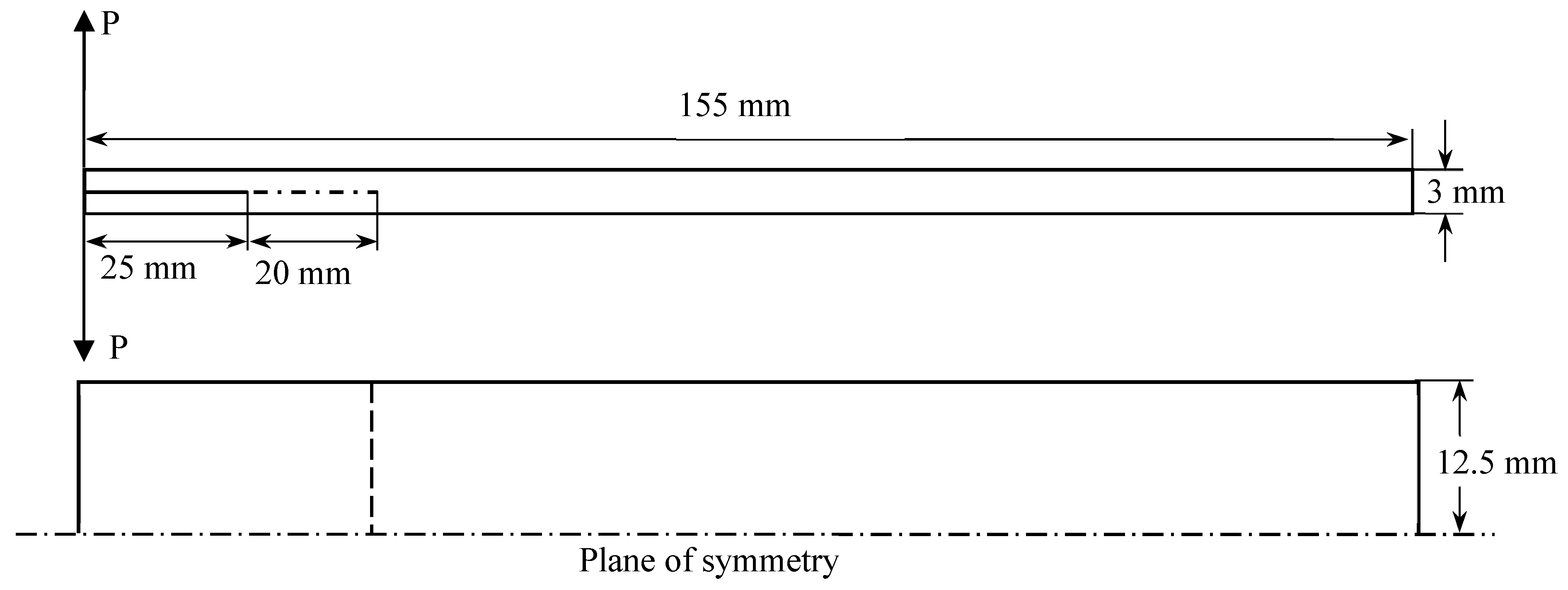
The model of DCB under loading symmetric about the delamination surface represents the experiment for determining the opening Mode I fracture toughness as defined by the standard test method [14]. The geometric dimensions of the DCB specimen are given in Figure 2. When generating the FE model, only the effective length of the specimen was taken into consideration. Specifically, 25 mm segments at the end of the specimen, where loading hinge tabs were attached, are not shown in the drawing in Figure 2, as they have not been modelled explicitly, to reduce the computational demands without affecting the results noticeably.
The initial delamination was represented by the 45 mm long segment, measured as a distance between the loading hinge and the delamination front in the mid-plane of the beam. This crack length was comprised of a 25 mm long segment, where the non-adhesive insert was placed to form an initiation site for delamination, which was propagated by 20 mm by applying the initial load as prescribed by the standard test procedure [14].
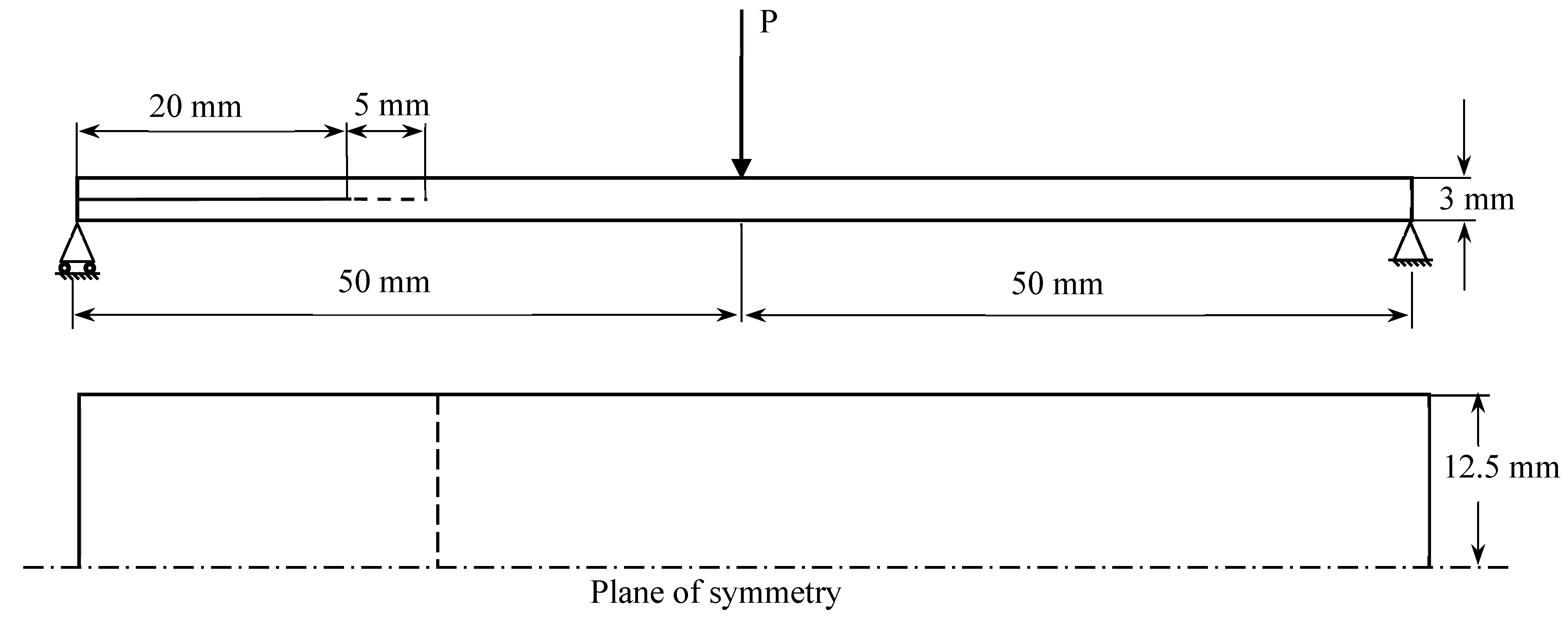
The Mode II model represents the end notched flexure (ENF) test according to its specification in standard [15]. The specimen was dimensioned as shown in Figure 3. Similar to Mode I model, only the effective length of the specimen, defined as the length between the supports, was modelled explicitly. The initial delamination length, in this case, was 25 mm, measured from the point of support to the delamination front, where 20 mm corresponded to the non-adhesive insert, which was propagated by 5 mm by applying the initial load with a slightly different setting to facilitate the process [15].
2.2. Finite Element Implementation
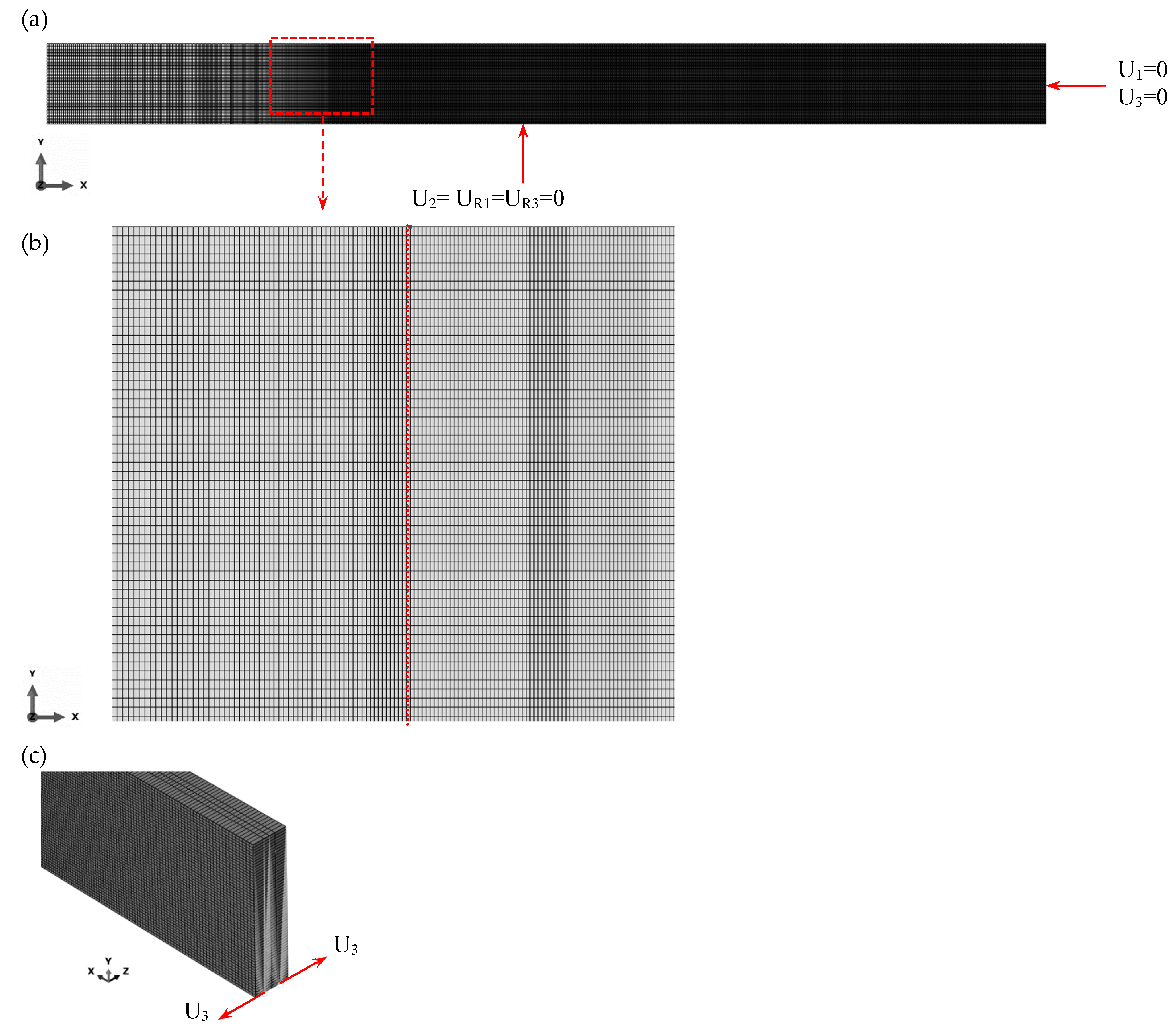
The meshed FE model employed for the simulation of Mode I test is shown in Figure 4. Due to the symmetry of the problem, only half of the DCB in the width direction was modelled to reduce the computational demands. Appropriate symmetry conditions, specified in Figure 4a, were imposed to the nodes on the symmetry plane. The rigid body displacement along the axis of the DCB, the deflection, and the rotation about the axis were constrained at the free end.
The loading was prescribed in a displacement controlled manner. Kinematic coupling constraint available in Abaqus [22] was applied to relate the displacements of all the nodes on the tip of each DCB leg to the displacement at a reference node, which was located in the centre of the end surface of each leg (hence on the symmetry plane), as shown in Figure 4c. The degree of freedom (dof) of the reference nodes representing the deflection were prescribed designated displacements as the mechanism of loading, in opposite directions to give Mode I delamination of the DCB. Three more dofs at each reference node, namely, the sideways displacement, rotation about the axis of the DCB, and that normal to the plane of the DCB had were constrained because of the symmetry of the structure, whilst the remaining two are left free.
It is worth noting that imposing the kinematic coupling constraint as described above is a good practice as it does not interfere with the rotation of the faces at the tips of the beam. These rotations occur due to the bending in the legs of the DCB in the experiments, which is what the hinges are meant to allow. Furthermore, the reactions can be readily obtained at the dofs of the two reference nodes where the deflections are prescribed. This allows for the construction of the load-displacement curve, which is the main output in the experiments, in a straightforward manner. Minimal post-processing is required. To account for the absolute delamination opening displacement, the difference of the two displacements (one positive and one negative) should be obtained taking account of the sense of these displacements. Since only half of the DCB has been modelled due to the symmetry, to recover the case for the full DCB, the load also needs to be doubled.
To simulate the ENF test, which produces a Mode II delamination scenario, the FE model was generated as shown in Figure 5. A major difference from the Mode I problem is the introduction of a contact condition between the entire surfaces of the sublaminates at the interface to prevent interpenetration of layers during the deformation process, as the two sublaminates tend to deflect towards the same direction. Similar to the Mode I model, the sideways displacement and rotations about the axes were constrained, and the displacement was prescribed at the reference point, marked in Figure 5, to simulate the loading. The reference point was connected to the nodes at the upper surface of the beam along the dotted line in the middle of the length of the beam as shown in Figure 5a. Equation constraints were employed to impose the connection. In order to obtain the load-displacement curve, the reaction and displacement output at the reference point were used, where the load was doubled to recover the full Mode II model.
In both models, sublaminates were meshed with continuum shell elements, SC8R. The uniform in-plane mesh was applied to the sublaminates in Mode II model while in Mode I model, to reduce the computational costs, the biased mesh was used on parts of the sublaminates on either side of the initial delamination zone, with mesh refining towards the delamination front. Henceforth, whenever mesh density in Mode I model is mentioned, it refers only to the part of the DCB with the uniform in-plane mesh.
Usually, a number of layers of continuum shell elements will be required for the sublaminate on either side of the delamination [26]. When refining mesh through the thickness of the beam, it is reasonable to employ mesh biased towards the interface on each side of it. In particular, when four sublaminates are employed, as for DCB in Figure 4c, their thicknesses were 1.0, 0.5, 0.5 and 1.0 mm from bottom to top with delamination plane lying in the middle.
The interface was modelled by a layer of cohesive elements, COH3D8, placed along the mid-surface of the beam. The element in-plane dimensions matched those of the adjacent sublaminates, whilst the geometric thickness of the cohesive layer was equal to zero. To account for the presence of initial delamination in the models, the cohesive elements were generated only over the initially undelaminated parts of the respective interfaces.
2.3. Definition of Material Behaviour
The constitutive behaviour of plies and interface was prescribed via the material models readily available in Abaqus [22]. Specifically, composite plies with unidirectional carbon fibre reinforcement were defined as a transversely isotropic elastic material, whilst the elastic behaviour of the interface was defined in terms of tractions, t, and separations, δ, relationship as
where T is the constitutive thickness of the cohesive element as introduced in Abaqus [22], to be distinguished from the geometric thickness which is defined as the distance between the nodes on the upper and lower surfaces of the cohesive element, and , and represent the stiffness characteristics of the interface in normal and two perpendicular tangential directions to the interface. In all FE models considered here, the constitutive interface thickness was prescribed a default value of unity, in which case the relative separation displacements are equal to nominal strains.
Damage initiation is governed by a quadratic interfacial traction criterion, which is defined as follows:
where , and are the peak nominal stresses in normal and tangential directions, and are the Macaulay brackets.
In terms of modelling the damage evolution, Abaqus offers displacement- and energy-based approaches, and three softening schemes, namely, linear, exponential and tabular softening. Due to the complexity of the problem of damage evolution, no conclusive evidence is available to date demonstrating advantages of any one of these approaches over the others in terms of reproducing the physical reality of the process. In the present paper, the linear softening scheme was adopted to define the damage variable, D, the evolution of which is derived based on a power law criterion for mixed mode delamination:
where , and are fracture energies and , and their critical values. The values of exponents in (3) were chosen as [27]. The schematic of traction-separation responses corresponding to the linear softening scheme is shown in Figure 6.
This approach to damage modelling is the one most commonly used in the literature, and, being adopted from fracture mechanics, it appears to have relevance to the physical reality of the delamination process. Further assessment of the applicability of the energy approach to delamination problems will be made in Section 4.3 of the present paper.
2.4. Definition of the Parameters of the Model
The mechanical properties for composite plies and interface layers, required to conduct the analysis, are summarised in Table 1. They correspond to composite laminates manufactured from commercial G827 carbon unidirectional (UD) cloth injected with bismaleimide resin (trade-name 6421), using resin transfer moulding (RTM). Most of the properties were provided in [25,28] as referenced in Table 1, yet they were insufficient to fully define the materials involved. To facilitate the modelling, the remaining properties were obtained making use of the composite characterisation tool, UnitCells©, developed at the University of Nottingham [29]. The detailed account as to how these parameters were obtained is given in [30].
In addition to material properties in Table 1, there is yet another set of parameters that must be specified to complete the definition of the model. These analysis-related parameters, which can only be obtained via the parametric sensitivity studies, are subdivided into two groups. The first one, given in Table 2, includes the dimensions/number of elements in the mesh, which are treated in the present study as the parameters of the model. Another group, summarized in Table 3, comprises some of the necessary input data for the cohesive model, including the interface stiffnesses, as introduced in the section ‘Definition of material behaviour’, which are essentially the penalty parameters, and the viscosity parameter, μ [22]. The latter is required in order to overcome the convergence difficulties which commonly occur when modelling materials with softening behaviour with Abaqus/Standard solver. Given their penalty sense, these parameters can all have a reasonable range within which the precise values will not make a noticeable difference. For this reason, they are shown in their orders of magnitude.
The mesh density and cohesive interface parameter values listed in Table 2 and Table 3, respectively, correspond to the converged results, which, for ease of reference, will be referred to as benchmark cases. Strictly speaking, the data shown are applicable to the material system as employed in this study. However, they should offer relevant guidance if different material systems are dealt with to avoid full spectrum search.
Inappropriate selection of the values of these parameters typically results in completely erroneous predictions and/or convergence difficulties, yet the only way to determine them is via the parametric convergence studies. These convergence studies will be the main subject of discussion in the next section as there has been a lack of such guidelines in the literature.
3. Studies on the Factors Affecting Convergence of the Cohesive Model
The convergence of the solution was assessed by comparing the load-displacement curves, which are typical outputs in both the Mode I and Mode II cases, obtained at different values of the parameters. In each parametric study, all parameters but one were kept fixed at the values given in Table 2 and Table 3 unless otherwise specified.
3.1. Mode I
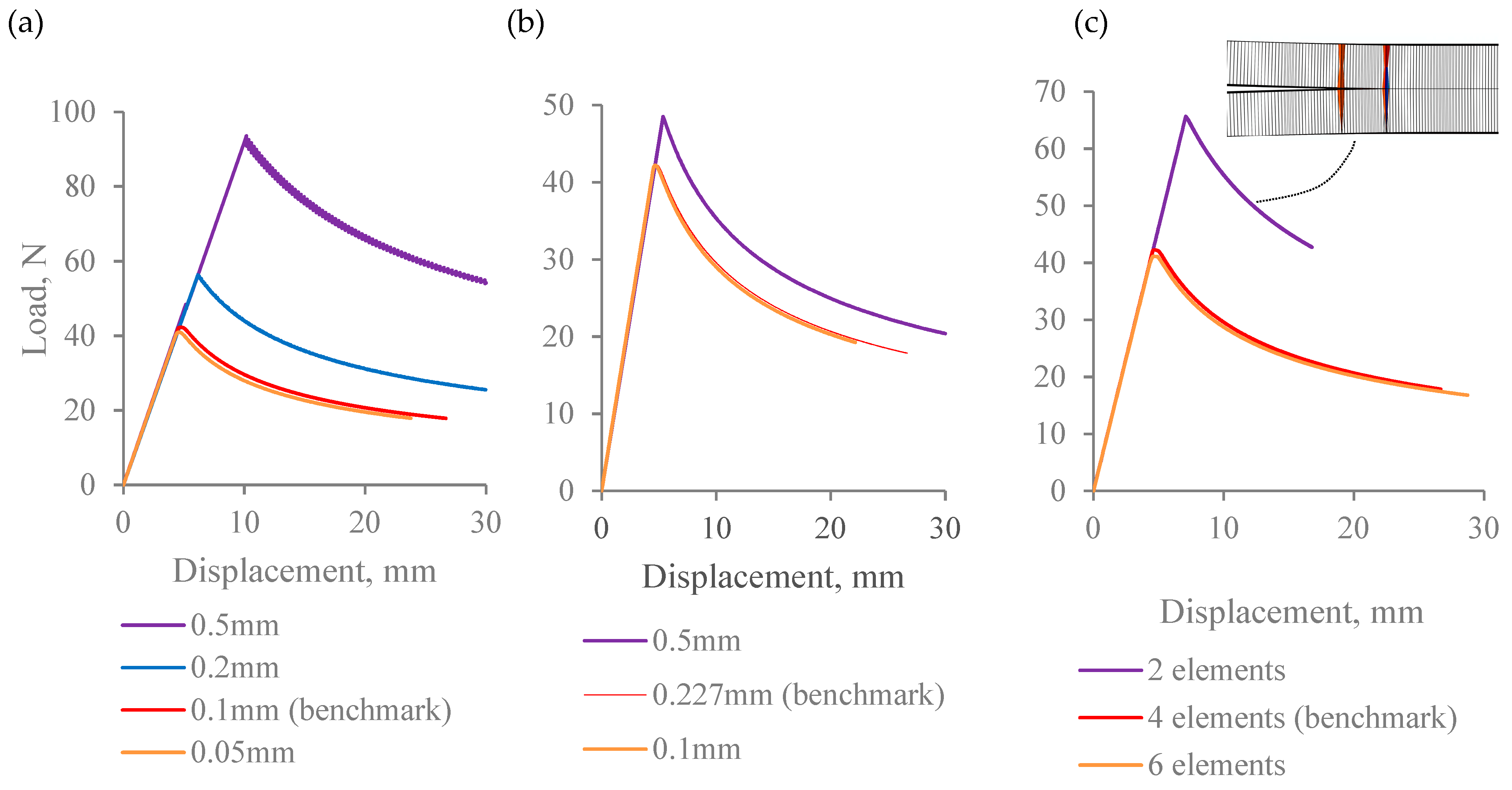
Given the high mesh sensitivity of delamination problems in general, the mesh refinement study was conducted first, where the size of elements was consecutively varied in length, width, and thickness direction. The calculated load-displacement corresponding to these cases is shown in Figure 7a–c, respectively. The most important observations from this mesh sensitivity study are summarized as follows:
- (i)
- Converged solution in Mode I simulation requires very fine meshing. This results in lengthy computational times, even with the use of high-performance computing. Specifically, the benchmark Mode I model contained over 350 K elements. Further mesh refinement substantially increased the computational demands, hence the load-displacement curves obtained at the smallest mesh size in Figure 7a,b were not computed for the full range.
- (ii)
- Insufficient mesh refinement in thickness direction results in convergence difficulties. The model with two elements in the thickness direction in Figure 7c, has shown a lack of convergence because of the distortion of continuum shell elements, as shown in sub-figure on the same plot. It has confirmed that the mesh, in this case, was not fine enough, hence the analysis was manually interrupted.
- (iii)
- It is apparent that whilst the results are sensitive to mesh density in all three directions, the most pronounced differences between the load-displacement curves were captured when the element size was varied along the length of the beam. In particular, with the largest element size considered, 0.5 mm along the length, the load values exceeded those in the converged solution by over 100%.
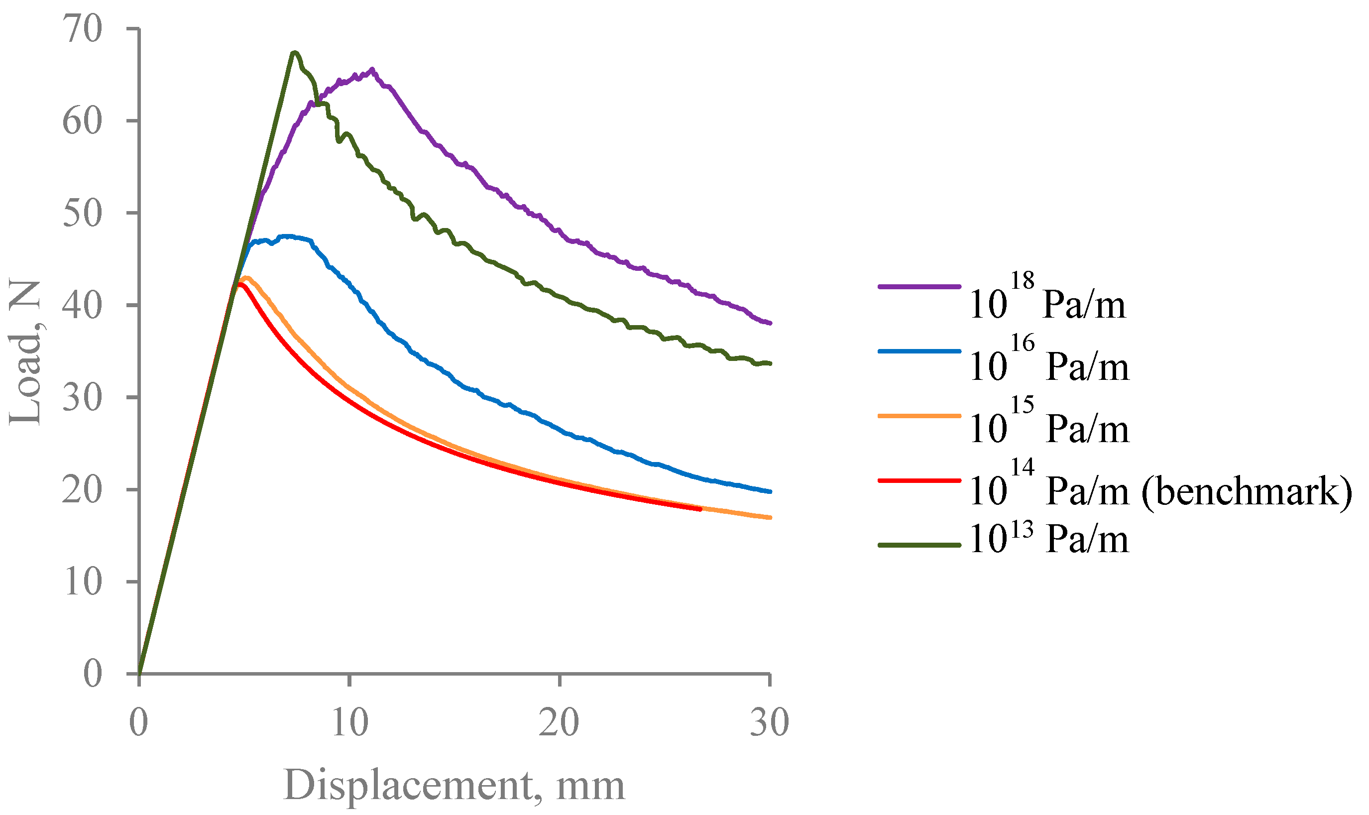
Similarly, the parametric study conducted with respect to the interface stiffness parameter has shown that it also has a significant effect on load-displacement predictions. Since shear stiffness terms do not contribute to delamination propagation in Mode I case, the study was conducted with respect to the normal stiffness component, which was varied over a reasonably wide range, with the results of the study being presented in Figure 8. As can be seen, the converged solution was obtained at 1014–1015 Pa/m, which, in fact, falls within the range recommended by Zou et al. [20]. Further increases of stiffness led to convergence issues following the delamination onset point, where the load-displacement curves were no longer smooth, and the peak load values were substantially overestimated. Similarly, reduction of the stiffness to values below those in this range resulted in the overestimation of the load and convergence issues.
The main point to emphasise here is that the mathematical identities of interface stiffnesses are penalty functions which are employed to impose certain constraints numerically. In particular, it is suggested that the interface stiffnesses are to be treated as penalty parameters in Abaqus Analysis User’s Guide [22]. The guideline for the selection of their values is therefore that they must be sufficiently large to ensure the constraints are imposed reasonably accurately, yet excessively large values could cause numerical ill-conditioning. The most reliable method for finding the right magnitude is via the parametric sensitivity study, as demonstrated here.
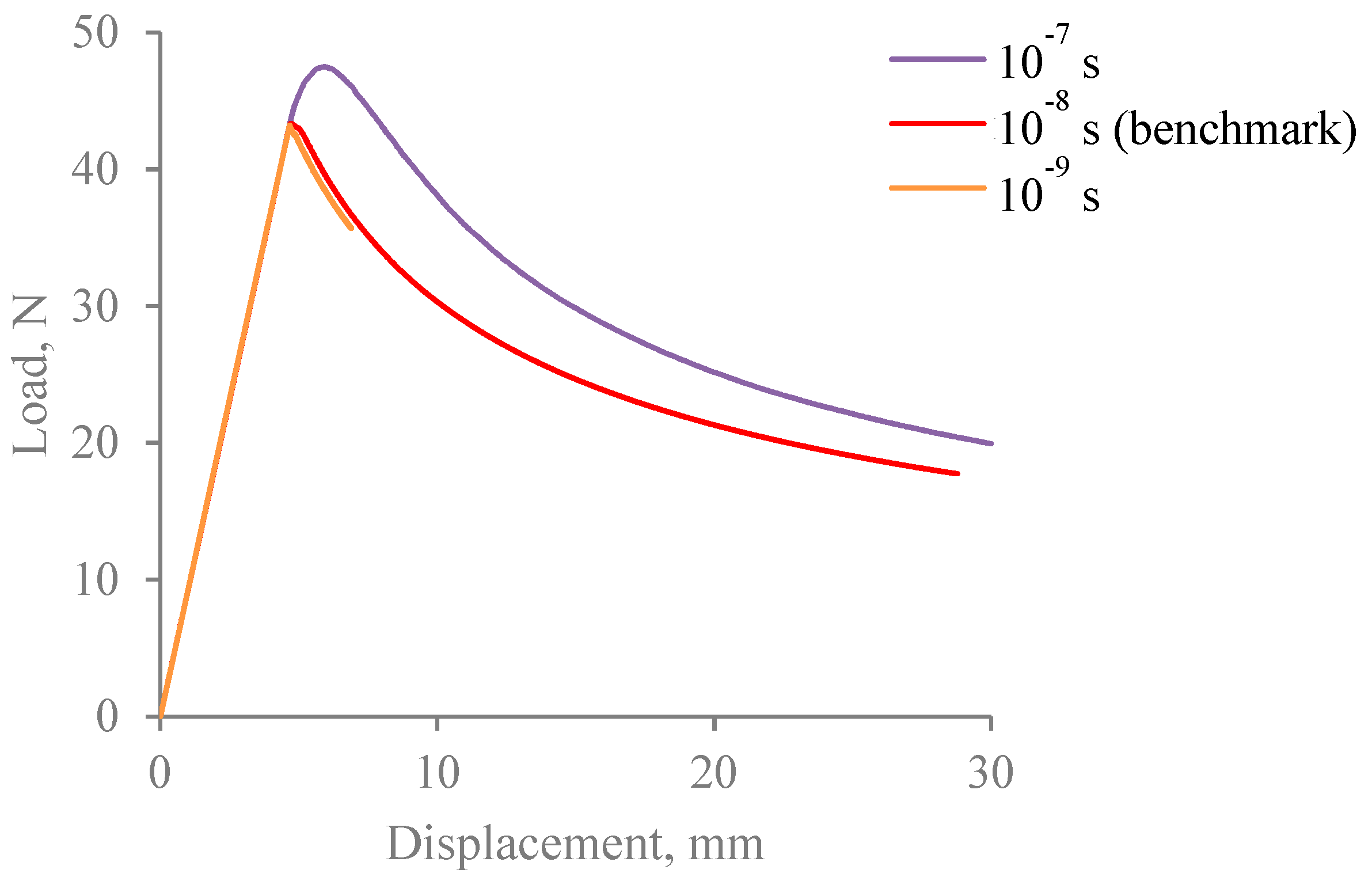
Definition of viscosity parameter in the simulations conducted was necessary to ensure convergence of the solution and successful completion of the analysis. The load-displacement curves obtained at different values of the viscosity parameter are shown in Figure 9. As can be seen, at μ = 10−7 s the results are compromised, as there is an apparent discrepancy between the corresponding curve and the converged solution. Conversely, the load-displacement curve obtained with μ = 10−9 s is very close to the converged one, yet such choice of a parameter appeared to be detrimental to the analysis, making it computationally costly. According to the recommendation given in the Abaqus Analysis User’s Guide, the value of viscosity should be small compared to the characteristic time increment. In the simulations carried out here, the time increment was not fixed, with its value varying in the range from 10−8 to 10−6 s. This indicates that the viscosity parameter should, in fact, be comparable to the time increment size.
It is also worth noting that, being related to the time increment size, the value of viscosity needs to be scaled accordingly if the step time is altered. Specifically, in all the analyses conducted in the present paper, step time value was defined as 10−3 s. Should it be altered, the viscosity value must be changed, too.
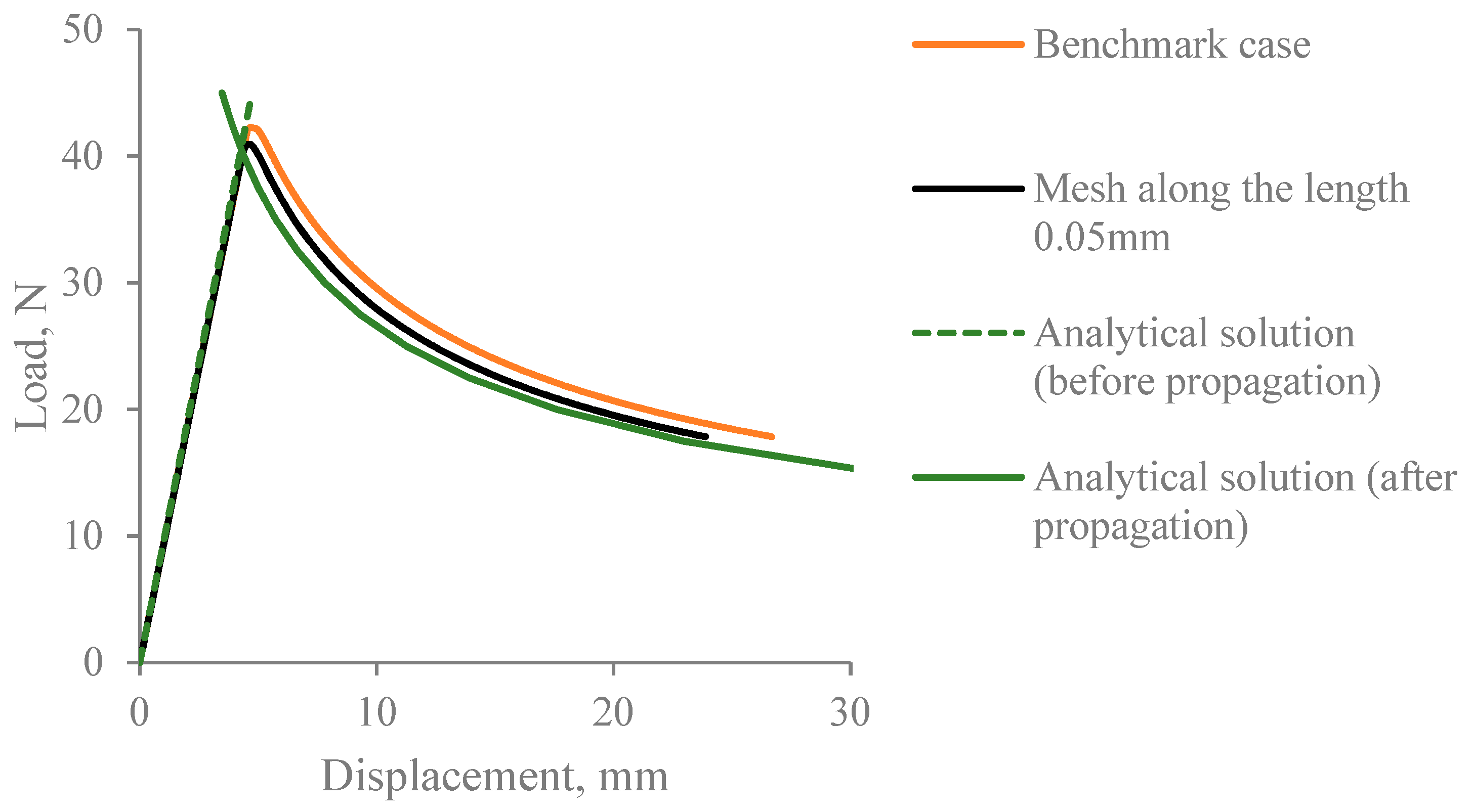
The parametric sensitivity studies presented demonstrate that the benchmark load-displacement curve indeed represents the converged solution. This conclusion can be further supported by comparison with the analytical solution in Figure 10, which shows a close agreement between the two. The solution used was derived in [20,31]. A close correspondence can be observed between the elastic parts of the curves. In this region, an analytical solution tends to deviate gradually from the calculated curve, predicting a slightly stiffer response. This can be attributed to the evolution of damage at the crack front that was predicted early on in the FE simulation. In the nonlinear part, there is a small discrepancy between the analytical and calculated curves, yet the two can be brought closer together by further mesh refinement.
3.2. Mode II
The sensitivity studies conducted with Mode I model were repeated for the ENF model, which led to the Mode II delamination scenario. The mesh refinement study for this case has shown that the results are generally insensitive to the sizes of elements along the length of the beam and in thickness direction over the range involved, as can be seen in Figure 11a,c, respectively, where the load-displacement curves are virtually the same. Unlike in Mode I simulations, where the longitudinal dimensions of the elements made the most pronounced difference to the results, the most significant variation in the results obtained with Mode II model was captured when the size of elements along the width of the beam is varied, as shown in Figure 11b.
The results of the parametric study with respect to the penalty shear stiffness parameter are presented in Figure 12. The normal stiffness term was kept fixed, as it did not contribute to delamination propagation in ENF model configuration. Unlike in the Mode I case, the load-displacement curves were hardly affected when the parameter value was increased by several orders of magnitude. Reducing the value of the penalty stiffness from the benchmark by two orders of magnitude led to a significant overestimation of the value of the peak load.
In terms of sensitivity to viscosity parameter, qualitatively, the Mode II model exhibits the same effects as were identified for the Mode I model. The load-displacement curves for this parametric study are shown in Figure 13. As can be seen, the reduction of the parameter below the converged value made only a marginal difference to the results, whilst increasing its value affected the load reduction part of the curve following the onset of delamination.
The converged solution gives the most representative behaviour of the cohesive model. It is compared with the analytical solution from [32] in Figure 14. The lower stiffness of the elastic part predicted in FE simulation is due to the use of continuum shell elements which allow transverse shear deformation, whilst the analytical solution is based on Bernoulli beam having infinite transverse shear stiffness. Given that the problem is transverse shear-dominated, the analytical solution is expected to predict higher stiffness. There is an apparent difference between the analytical and converged FE solution after delamination propagation takes place. The former one exhibits a reduction of the force while the displacement reduces. This is different from elastic unloading as the process is accompanied by unstable delamination propagation. Equilibrium states of this kind are usually extremely unstable and the instability cannot be helped even if the loading mode is kept under displacement control. Experimentally, under displacement control, what one usually observes is a sharp drop in load accompanied by a rapid delamination growth to a level when the specimen is capable of sustaining the load in a stable manner as is illustrated in Figure 14 as purple dashed line. The converged FE solution indeed shows a rapid drop of the load at almost a constant displacement which was obtained under displacement control.
3.3. Implications of Insufficient Mesh Refinement
The effects of insufficient mesh refinement on damage contours at delamination front in Mode I and Mode II models are illustrated by Figure 15b,d, respectively, whilst those in Figure 15a,c correspond to the respective benchmark cases. As can be seen, the lack of mesh refinement along the length of the Mode I model leads to forming of a localised bulge at the delamination front, instead of the well-known fingernail shape as in benchmark case. Sawtooth damage pattern at the delamination front was captured for the Mode II model with insufficient mesh refinement along the width of the beam.
It is worth noting that distortion of the damage contours at the delamination front is not necessarily accompanied by a significant deviation of the load-displacement curves from those obtained for the converged benchmark cases. Specifically, for the Mode II case, the curve associated with the damage contour in Figure 15d is plotted in Figure 11b (blue line). As can be seen, it is very similar to that in the converged case.
3.4. Cohesive Surface as an Alternative Presentation of the Cohesive Zone Model
An alternative method of defining the cohesive behaviour is via the use of surface-based presentation, which is defined as a surface interaction property. It is yet another capability readily available in Abaqus. It involves specification of generalized traction-separation behaviour for surfaces, formulation of which is identical to that available for the cohesive elements. Therefore, cohesive surfaces are often used as an alternative for cohesive elements when studying the delamination problems. However, to date, no comprehensive direct comparison between the two was reported. To fill this gap, Mode I and Mode II simulations were conducted, where the surface-based cohesive interaction was employed to model delamination at the interface.
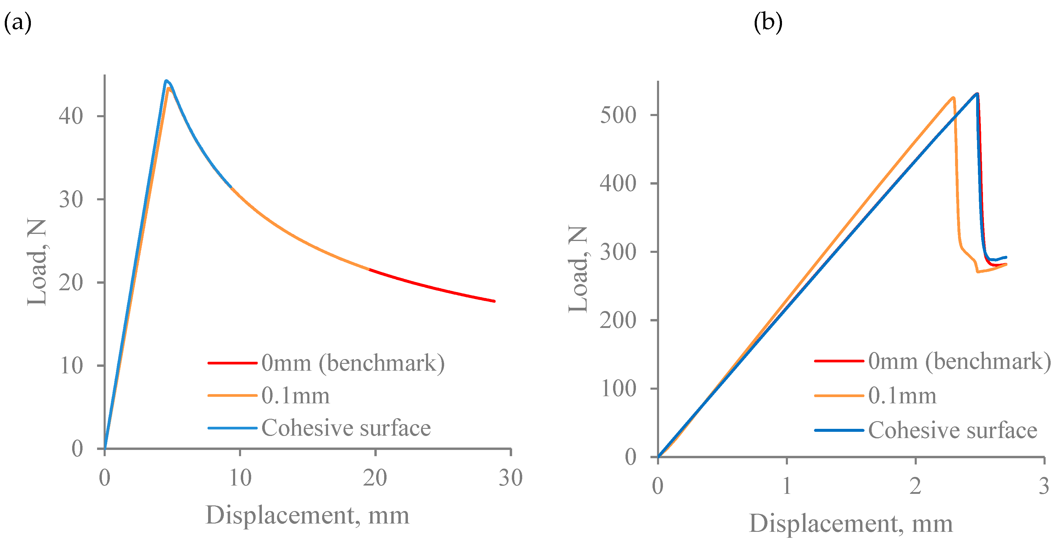
The load-displacement curves calculated for Mode I and Mode II cases with surface-based cohesive interaction are presented in Figure 16a,b, respectively. For comparison, the curves corresponding to the benchmark cases were also included in the plots. As can be seen, the use of cohesive surfaces and cohesive elements result in virtually the same predictions. Minor discrepancies between the two curves are observed near the peak load in Mode I, and for the part of the curve corresponding to the propagation of delamination in Mode II.
3.5. Geometric Thickness of the Interface
The surface-based cohesive behaviour does not account for the interface geometric thickness effects, unlike the cohesive elements, for which geometric thickness can be non-zero. This makes interface thickness yet another parameter, the influence of which on modelling results is unclear. The description given in the Abaqus Analysis User’s Guide [22] as to how the thickness of cohesive elements should be defined does not provide a straightforward recipe to follow in this respect.
In all the simulations presented, the geometric thickness of the interface was equal to zero. In order to check whether it has any effect on the predictions, another set of Mode I and Mode II models was generated, in which the geometric interface thickness was equal to 0.1 mm, and the load-displacement curves were compared to those corresponding to benchmark cases.
Results in Figure 16a show that in Mode I case, the load-displacement curve obtained for the model with a 0.1 mm-thick interface was found to be identical to the benchmark one. On the other hand, in Mode II, there is a substantial discrepancy between the two curves, as can be seen in Figure 16b. In this case, whilst the predicted peak loads were nearly the same, the slope of the linear part of the curve calculated employing cohesive elements of 0.1 mm geometric thickness has become steeper compared to the benchmark case.
4. Verification Based on the Critical Energy Release Rates
The main objective of conducting standard Mode I and Mode II tests [9,10,14,15] is to determine the respective fracture toughnesses. Their experimental values served as input in Mode I and Mode II simulations. It is natural to expect that the energy release rates extracted from the results should, in turn, reproduce the input values through the corresponding simulations, if the models are a truthful representation of the physics, with the simulations considered as virtual testing. An exercise of this kind would serve as a ‘sanity check’ on the representativeness of the model employed, i.e., the cohesive model in the context of the present paper. Of course, to be practically meaningful, any assessment should be based on duly converged solutions. The converged solution is unique to the numerical tolerance allowed, whilst the non-converged one can be anything, numerous examples of which were given in the previous section. To ensure the comparisons are made like with like, the critical energy release rates were evaluated by post-processing the results according to the appropriate standard procedures [9,10,14,15].
4.1. Mode I
According to standards [9] and [14], the delamination length readings should be recorded continuously throughout the test, as they were required in order to work out Mode I fracture toughness.
To determine the delamination length, the results were post-processed via the use of the Python script, extracting the length of delamination at each increment by calculating the distance between the initial and the current delamination front. Thus, the extracted delamination length is plotted in Figure 17 (solid grey) as a function of the opening displacement.
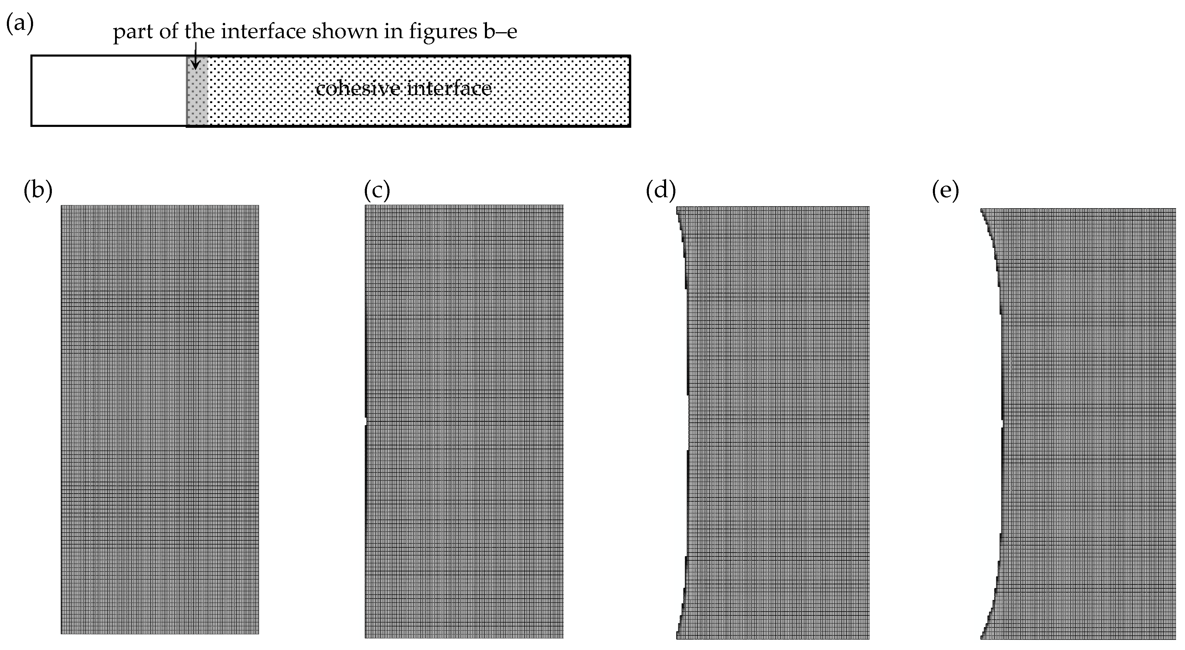
In terms of calculations, the two standards referred to use different methods for evaluating the fracture toughness. Specifically, the expression given in [9] requires measurement of the load and displacement at the onset of delamination movement. When extracting these from the results, one ought to bear in mind that the initial delamination front in the model that is not a truthful reflection of that in the test. Consider typical predicted delamination front propagation in Figure 18, where part of the interface near the delamination front is shown, with the symmetric half recovered. Initially, it is straight, as shown in Figure 18b. Once the delamination is triggered (Figure 18c), it starts propagating from the middle of the interface, spreading outwards to both edges (Figure 18d). The pattern becomes established when it starts to propagate at the edges of the beam (Figure 18e). This thumbnail shape for delamination front is due to anticlastic effects in the bent legs of the DCB, and it is consistently reproduced in Mode I DCB tests [33].
On the other hand, the initial delamination in the experiments was induced via pre-loading, hence the delamination front had the characteristic curved shape. Therefore, the Mode I results begin to reproduce the experiment only when the delamination front becomes established. Load and displacement values at this point, marked as (d) on the inset inside Figure 17, should be used for calculating the critical energy release rate following the procedure given in [9].
Precisely following the procedures as provided in standards [9] and [14], the critical energy release rates were obtained from the present simulations treated as virtual testing. Their values are listed in Table 4 along with the experimental one used as the input for the simulation. Quantitatively, both standards give similar estimates of the energy release rates, which are nearly 15% higher than the input value. This discrepancy can be brought down by processing the case where mesh in the length direction was more refined. The mesh sensitivity study presented in section ‘Mode I’ has shown that the predictions are very sensitive to mesh size along the length of the beam, and the mesh refinement leads to the reduction of the peak load, as well as the load values past the delamination onset point in general (see Figure 7a). The mesh in a benchmark case was chosen as a compromise between the accuracy and computational efficiency, yet the analysis presented here suggests that it may still not be fine enough if the objective is to reproduce the input critical energy release rate. The data in Table 4 indicates that halving the mesh size in length direction brings the energy release rate closer to the experimental data, yet the estimates still remain higher than the measured value. Any further mesh refinement will not be computationally effective practically. It is not absolutely certain that infinite refinement would eventually reproduce the input exactly. It is perhaps a point when the user will have to make a subjective judgement whether an error of less than 10% should be considered as a lack of full convergence or lack of representativeness of the cohesive model.
In addition, there is a disparity between the simulated and experimental results exhibiting a thumbnail-shaped delamination front and the ideally straight delamination front as assumed in the standards, which dictates the way how experimental data should be processed. This undermines the perfect representativeness of the standard. One way or another, users should expect this level of numerical error involved in the numerical simulation of the delamination problem using the cohesive model even for this least controversial case. Realistically, for any practical application to more sophisticated problems, users should be prepared for larger margins of error. Any prediction more accurate than this cannot be considered as a genuine claim.
4.2. Mode II
The Mode II energy release rate was extracted from the results obtained in Mode II simulation, according to the procedures specified in standards [10] and [15]. Their values are given in Table 5. In this case, predictions are substantially closer to the experimental (input) values, especially those obtained following [10].
For the Mode II model, there is a further factor which has not been covered yet. As it has been demonstrated in a number of publications, friction between the delaminated surfaces sometimes makes a subtle difference to the results. In terms of modelling, the frictional behaviour can easily be accounted for by prescribing the tangential behaviour to the contacting surfaces through the definition of a single dimensionless friction coefficient, making use of the option available in Abaqus [22]. The parametric study where the value of the friction coefficient was varied is presented in Figure 19. The results indicate that the presence of friction marginally delays the onset of delamination, leading to the increase in values of the peak load, which is one of the key parameters when determining the energy release rate from ENF tests. The results in Table 5 show that incorporating a small amount of friction substantially improves the agreement between the measured values energy release rates calculated according to standard [15].
It is worth noting that the parametric study with respect to the friction parameter, as presented here, is different from those presented in section ‘Studies on the factors affecting convergence of the cohesive model’, since friction represents mechanical behaviour that can be quantified physically [34] whereas the parameters studied in that section are penalty parameters which can only be determined numerically via the convergence studies by means of trial and error.
As the results derived from standard [15] tend to approach the experimental value from below, incorporation of a small amount of friction seems to help reproduce the experimental value more closely. However, those derived from standard [10] cannot be helped as they seem to approach the experimental value from above and any consideration of friction would drive it further apart. Given that friction is an unavoidable physical reality, the accuracy achieved by the benchmark case seems more a coincidence than perfect representativeness.
Here, it is a point of reflection. Apparently, the same data processed according to different standards produce slightly different estimates for the same material property. This dismisses the possibility of a so-called perfect representation, no matter how realistic and accurate the theoretical model is. For more sophisticated applications, room should be allowed for accommodating errors due to imperfect representativeness of the cohesive model.
4.3. Critical Assessment of the Cohesive Model in General Applications to the Delamination Problem
The message conveyed through the ‘sanity checks’ as presented in the previous subsections is as follows. The cohesive model represents the delamination problem in its pure Mode I and Mode II scenarios reasonably accurately, provided that the convergence was reached in all relevant aspects as explored in Section 3. However, its representativeness even for these simple and the least controversial cases is not perfect and errors are expected beyond the convergence considerations. In other words, whilst a solution converges to a solution of some kind, the solution may well be one to a somewhat different problem.
The lack of representativeness of any delamination model, including CZM, will become even more apparent, and the relevance of available standards will be further undermined as soon as the application steps beyond the simplistic cases as involved in the previous sections, given the scenarios as depicted in Figure 1. The following issues are responsible for this:
- Critical energy release rates are measured in the experiments under very restrictive conditions: (i) Delamination takes place between laminae of the same fibre orientation; (ii) delamination propagates in the fibre direction; (iii) effects of finite specimen width are not accounted for when conducting the measurements. Data obtained under such conditions are far from being sufficient to cover all practical scenarios. For instance, one can easily differentiate the efforts required to propagate a crack in a UD composite along the direction of the fibres, referring to Figure 1a, and a different direction, referring to Figure 1b, let alone interlaminar delamination propagating in a direction different from fibre directions in the laminae on either side of the delamination, as illustrated in Figure 1c. Apparently, the scope of applicability has been blindly extrapolated when the same set of critical energy release rates is assumed for all delamination propagating in any direction.
- The evolution criterion (3) has been rather arbitrarily equipped. It was adopted from the fracture mechanics, but even in fracture mechanics no conclusive agreement has been reached about what power value was to be employed, linear or quadratic, let alone any other possible combinations. One set of them defines one problem and another set is applicable for another problem.
Each of these considerations results in the model deviating further from the intended problem and yet none of them have ever been properly scrutinised. This indicates that the state-of-the-art of the development is far from being satisfactory. Delamination modelling should not be turned into a black box before fundamental issues like these get clarified. Until then, it would be extremely hard to assess how close or distant the current treatments of delamination problem represent the reality. In this regard, designated investigations on the verification of delamination models should be encouraged, rather than be perceived as a low-key development.
5. Conclusions
Virtual testing has been conducted in this paper using CZM for the cases of Mode I and Mode II delamination as the two pure mode cases, which are meant to be the most straightforward types of delamination. Verification exercises referred to as ‘sanity checks’ were carried out to assess the representativeness of such a theoretical model of the physical delamination problem. Whilst the results draw close relevance of the model in terms of accuracies when compared to the analytical solutions of the two pure mode cases, the verification exercise outcomes indicate that the representativeness is questionable even for these simple cases. For general applications, more representative models are required, but the challenges lie not only in the modelling capability but also in more fundamental issues. These include, in particular, the definition of critical energy release rates for genuine interlaminar delamination with an arbitrary direction of delamination propagation. Revision of the fundamental concepts will inevitably require revision of associated testing standards.
Before perfectly representative delamination models become available, the user has to ensure when employing modern CZMs that the general convergence is achieved. This includes not only the conventional convergence of the FE mesh, but also a range of other issues as explored in this paper, such as convergence with respect to the various parameters of the model. Only then, the solution would be a genuine solution, even though it could be for a different problem. Before the general convergence is reached, the solution obtained will not even be a solution to any meaningful problem. The comprehensive guidelines for achieving the converged solution with CZM have been presented in this paper, eliminating all the misconceptions regarding the treatment of various aspects of the model that are often encountered in the literature.
Author Contributions
Conceptualization, S.L.; methodology, S.L. and E.S.; formal analysis, E.S. and D.L.; investigation, E.S., D.L. and S.L.; resources, J.W., X.Y.; data curation, J.W., X.Y.; writing—original draft preparation, E.S.; writing—review and editing, E.S., S.L.; supervision, E.S., S.L.; project administration, S.L., J.W. and X.Y.; funding acquisition, S.L., J.W. and X.Y.
Funding
This research was supported by a doctoral grant from the Beijing Institute of Aeronautical Materials (BIAM), China under Contract Number RGS 107903.
Conflicts of Interest
The authors declare no conflict of interest.
References
- FAA. Composite Aircraft Structure, Federal Aviation Administration Advisory Circular; AC No:20-107B; FAA: Washington, DC, USA, 2010.
- Barenblatt, G.I. The Mathematical Theory of Equilibrium Cracks in Brittle Fracture. In Advances in Applied Mechanics; Dryden, H.L., Ed.; Elsevier: Amsterdam, The Netherlands, 1962; pp. 55–129. [Google Scholar]
- Dugdale, D.S. Yielding of steel sheets containing slits. J. Mech. Phys. Solids 1960, 8, 100–104. [Google Scholar] [CrossRef]
- Yu, R.C.; Pandolfi, A. 15—Modeling of delamination fracture in composites: A review A2—Sridharan, Srinivasan. In Delamination Behaviour of Composites; Woodhead Publishing: Cambridge, UK, 2008; pp. 429–457. [Google Scholar]
- Hongkarnjanakul, N.; Bouvet, C.; Rivallant, S. Validation of low velocity impact modelling on different stacking sequences of CFRP laminates and influence of fibre failure. Compos. Struct. 2013, 106, 549–559. [Google Scholar] [CrossRef] [Green Version]
- ASME. Guide for Verification and Validation in Computational Solid Mechanics; An overview of the PTC 60/V&V 10; ASME: New York, NY, USA, 2006. [Google Scholar]
- Li, S.; Sitnikova, E. An Excursion into Representative Volume Elements and Unit Cells. In Reference Module in Materials Science and Materials Engineering; Elsevier: Amsterdam, The Netherlands, 2018. [Google Scholar]
- Li, S. On the unit cell for micromechanical analysis of fibre-reinforced composites. Proc. R. Soc. Lond. Ser. A Math. Phys. Eng. Sci. 1999, 455, 815. [Google Scholar] [CrossRef]
- ASTM International. ASTM Standard D5528-13: Standard Testing Method for Mode I Interlaminar Fracture Toughness of Unidirectional Fiber-Reinforced Polymer Matrix Composites; ASTM International: West Conshohocken, PA, USA, 2013. [Google Scholar]
- ASTM International. ASTM Standard D7905/D7905M-14: Standard Test Method for Determination of the Mode II Interlaminar Fracture Toughness of Unidirectional Fiber-Reinforced Polymer Matrix Composites; ASTM International: West Conshohocken, PA, USA, 2014. [Google Scholar]
- The British Standards Institution. BS EN 6033:2015: Aerospace Series—Carbon Fibre Reinforced Plastics—Test Method—Determination of Interlaminar Fracture Toughness Energy—Mode I—GIC; The British Standards Institution: London, UK, 2015. [Google Scholar]
- The British Standards Institution. BS EN 6034:2015: Aerospace Series—Carbon Fibre Reinforced Plastics—Test Method—Determination of Interlaminar Fracture Toughness Energy—Mode II—GIIC; The British Standards Institution: London, UK, 2015. [Google Scholar]
- ISO. International Standard ISO 15024:2001: Fibre-Reinforced Plastic Composites—Determination of Mode I Interlaminar Fracture Toughness, GIC, for Unidirectionally Reinforced Materials; ISO: Geneva, Switzerland, 2001. [Google Scholar]
- Standard of Chinese Aviation. HB 7402-96: Testing Method for Mode I Interlaminar Fracture Toughness of Carbon Fiber Reinforced Plastics. Available online: https://news.efucai.net/article/pro/details?articleId=5573 (accessed on 27 February 2019).
- Standard of Chinese Aviation. HB 7403-96: Testing Method for Mode II Interlaminar Fracture Toughness of Carbon Fiber Reinforced Plastic. Available online: https://news.efucai.net/article/pro/details?articleId=4993 (accessed on 27 February 2019).
- Sitnikova, E.; Li, S.; Li, D.; Yi, X. Subtle features of delamination in cross-ply laminates due to low speed impact. Compos. Sci. Technol. 2017, 149, 149–158. [Google Scholar] [CrossRef]
- Turon, A.; Dávila, C.G.; Camanho, P.P.; Costa, J. An engineering solution for mesh size effects in the simulation of delamination using cohesive zone models. Eng. Fract. Mech. 2007, 74, 1665–1682. [Google Scholar] [CrossRef]
- Harper, P.W.; Hallett, S.R. Cohesive zone length in numerical simulations of composite delamination. Eng. Fract. Mech. 2008, 75, 4774–4792. [Google Scholar] [CrossRef] [Green Version]
- Alfano, G.; Crisfield, M.A. Finite element interface models for the delamination analysis of laminated composites: Mechanical and computational issues. Int. J. Numer. Methods Eng. 2001, 50, 1701–1736. [Google Scholar] [CrossRef]
- Zou, Z.; Reid, S.R.; Li, S. A continuum damage model for delaminations in laminated composites. J. Mech. Phys. Solids 2003, 51, 333–356. [Google Scholar] [CrossRef]
- Camanho, P.P.; Davila, C.G.; De Moura, M.F. Numerical Simulation of Mixed-Mode Progressive Delamination in Composite Materials. J. Compos. Mater. 2003, 37, 1415–1438. [Google Scholar] [CrossRef]
- ABAQUS Inc. Abaqus Analysis User’s Guide; Abaqus 2016 HTML Documentation; ABAQUS Inc.: Alto, CA, USA, 2016. [Google Scholar]
- Barbero, E.J. Finite Element Analysis of Composite Materials Using ABAQUS; CRC Press, Taylor & Francis Group: Boca Raton, FL, USA, 2013. [Google Scholar]
- Girão Coelho, A.M. Finite Element Guidelines for Simulation of Delamination Dominated Failures in Composite Materials Validated by Case Studies. Arch. Comput. Methods Eng. 2016, 23, 363–388. [Google Scholar] [CrossRef]
- Cheng, Q.; Fang, Z.; Yi, X.-S.; An, X.; Tang, B.; Xu, Y. “Ex situ” concept for toughening the RTMable BMI matrix composites, Part. I: Improving the interlaminar fracture toughness. J. Appl. Polym. Sci. 2008, 109, 1625–1634. [Google Scholar] [CrossRef]
- Zou, Z.; Reid, S.R.; Soden, P.D.; Li, S. Mode separation of energy release rate for delamination in composite laminates using sublaminates. Int. J. Solids Struct. 2001, 38, 2597–2613. [Google Scholar] [CrossRef]
- Charalambides, M.; Kinloch, A.J.; Wang, Y.; Williams, J.G. On the analysis of mixed-mode failure. Int. J. Fract. 1992, 54, 269–291. [Google Scholar]
- Cheng, Q.; Fang, Z.; Yi, X.-S.; An, X.; Tang, B.; Xu, Y. Ex-situ concept for toughening the RTMable BMI matrix composites. II. Improving the compression after impact. J. Appl. Polym. Sci. 2008, 108, 2211–2217. [Google Scholar] [CrossRef]
- Li, S.; Jeanmeure, L.F.C.; Pan, Q. A composite material characterisation tool: UnitCells. J. Eng. Math. 2015, 95, 279–293. [Google Scholar] [CrossRef]
- Li, D.; Sitnikova, E.; Li, S.; Yi, X. Modelling Damage due to Low Speed Impact in Laminated Composites of Toughened Interfaces through ‘Ex Situ’ Technique. In Proceedings of the 20th International Conference on Composite Materials, Copenhagen, Denmark, 19–24 July 2015. [Google Scholar]
- Zou, Z.; Reid, S.R.; Li, S.; Soden, P.D. General expressions for energy–release rates for delamination in composite laminates. Proc. R. Soc. Lond. Ser. A Math. Phys. Eng. Sci. 2002, 458, 645. [Google Scholar] [CrossRef]
- Carlsson, L.A.; Gillespie, J.W. Chapter 4—Mode-II Interlaminar Fracture of Composites. In Composite Materials Series; Friedrich, K., Ed.; Elsevier: Amsterdam, The Netherlands, 1989; pp. 113–157. [Google Scholar]
- Jiang, Z.; Wan, S.; Zhong, Z.; Li, M.; Shen, K. Determination of mode-I fracture toughness and non-uniformity for GFRP double cantilever beam specimens with an adhesive layer. Eng. Fract. Mech. 2014, 128, 139–156. [Google Scholar] [CrossRef]
- Schön, J. Coefficient of friction of composite delamination surfaces. Wear 2000, 237, 77–89. [Google Scholar] [CrossRef]
Figure 1.
Schematics of potential scenarios of delamination front propagation: (a) delamination is between laminae of the same fibre orientation with the direction of propagation being along the fibres; (b) delamination is between laminae of the same fibre orientation but the direction of propagation is different from the fibre direction; and (c) delamination between laminae of the different fibre orientations.

Figure 2.
The geometry of double cantilever beam (DCB) specimen in Mode I tests.

Figure 3.
Effective dimensions of the specimen in Mode II tests.

Figure 4.
FE model for simulating Mode I experiment: (a) in-plane meshing of the model and constraints; (b) the mesh near the crack front marked by the red dashed line; (c) through-thickness mesh and kinematic coupling constraint at the tip of the DCB.
Figure 4.
FE model for simulating Mode I experiment: (a) in-plane meshing of the model and constraints; (b) the mesh near the crack front marked by the red dashed line; (c) through-thickness mesh and kinematic coupling constraint at the tip of the DCB.

Figure 5.
FE model for simulating Mode II experiment: (a) top view; (b) front view.

Figure 6.
Linear softening scheme adopted in the present study.

Figure 7.
The load-displacement curves for Mode I loading when mesh density varies (a) along the length of the beam; (b) along the width of the beam; (c) in the thickness direction.
Figure 7.
The load-displacement curves for Mode I loading when mesh density varies (a) along the length of the beam; (b) along the width of the beam; (c) in the thickness direction.

Figure 8.
Sensitivity of load-displacement predictions to the normal interface stiffness.

Figure 9.
Parametric study with respect to the viscosity parameter.

Figure 10.
Comparison of the converged solution obtained via FE modelling with an analytical solution from [20,31].

Figure 11.
Mesh sensitivity study for the Mode II model, when the mesh is refined (a) along the length of the beam; (b) along the width of the beam; and (c) in a thickness direction.
Figure 11.
Mesh sensitivity study for the Mode II model, when the mesh is refined (a) along the length of the beam; (b) along the width of the beam; and (c) in a thickness direction.

Figure 12.
Sensitivity of load-displacement predictions in the Mode II model to value of the penalty shear stiffness.
Figure 12.
Sensitivity of load-displacement predictions in the Mode II model to value of the penalty shear stiffness.

Figure 13.
Influence of viscosity on load-displacement predictions obtained with Mode II model.

Figure 14.
Comparison of the converged solution for Mode II obtained via FE modelling with an analytical solution from [32].
Figure 14.
Comparison of the converged solution for Mode II obtained via FE modelling with an analytical solution from [32].

Figure 15.
Damage contours at the delamination fronts (half width): (a) benchmark case for the Mode I model; (b) Mode I model with element size 0.5 mm along the length; (c) benchmark case for Mode II model; (d) Mode II model with element size 0.5 mm along the width.
Figure 15.
Damage contours at the delamination fronts (half width): (a) benchmark case for the Mode I model; (b) Mode I model with element size 0.5 mm along the length; (c) benchmark case for Mode II model; (d) Mode II model with element size 0.5 mm along the width.

Figure 16.
Load-displacement curves at different interface thicknesses and types of the interface layer: (a) Mode I simulation; (b) Mode II simulation.
Figure 16.
Load-displacement curves at different interface thicknesses and types of the interface layer: (a) Mode I simulation; (b) Mode II simulation.

Figure 17.
Simulated Mode I load and delamination length versus opening displacement.

Figure 18.
Shape at delamination front in Mode I simulation: (a) schematic of DCB specifying the part of the interface to be examined; (b) initial delamination front; (c) onset of delamination propagation; (d) delamination propagation towards the edges; (e) established delamination front.
Figure 18.
Shape at delamination front in Mode I simulation: (a) schematic of DCB specifying the part of the interface to be examined; (b) initial delamination front; (c) onset of delamination propagation; (d) delamination propagation towards the edges; (e) established delamination front.

Figure 19.
Load-displacement curves in Mode II simulations at a range of friction values.


Table 1.
Laminar mechanical properties.
| Longitudinal tensile modulus, E1 (GPa) | 102 [28] |
| Transverse tensile modulus E2 = E3 (GPa) | 4.8 |
| Longitudinal shear modulus G12 = G13 (GPa) | 2.0 |
| Transverse shear modulus G23 (GPa) | 1.7 |
| Longitudinal Poisson’s ratio, ν12 | 0.32 [28] |
| Transverse Poisson’s ratio ν23 | 0.42 |
| Interlaminar tensile strength, σc (MPa) | 67.6 [25] |
| Interlaminar shear strength, τc (MPa) | 103 [28] |
| GIc (J/m2) | 215 [25] |
| GIIc = GIIIc (J/m2) | 510 [25] |
Table 2.
Mesh density at which converged solution is obtained.
| Element direction | Mode I | Mode II |
|---|---|---|
| Element size/number along the length of the model | 0.1 mm/1100 elements | 0.2 mm/500 elements |
| Element size/number along the width of the model | ≈0.227 mm/55 elements | 0.2 mm/63 elements |
| Number of elements in through-thickness direction | 4 | 2 |
Table 3.
Properties of the cohesive interface at which converged solution is obtained.
| Penalty stiffness | Knn = Kss = Ktt = 1014 Pa/m |
| Viscosity parameter | 10−8 s |
© 2019 by the authors. Licensee MDPI, Basel, Switzerland. This article is an open access article distributed under the terms and conditions of the Creative Commons Attribution (CC BY) license (http://creativecommons.org/licenses/by/4.0/).
Share and Cite
MDPI and ACS Style
Sitnikova, E.; Li, D.; Wei, J.; Yi, X.; Li, S. On the Representativeness of the Cohesive Zone Model in the Simulation of the Delamination Problem. J. Compos. Sci. 2019, 3, 22. https://0-doi-org.brum.beds.ac.uk/10.3390/jcs3010022
AMA Style
Sitnikova E, Li D, Wei J, Yi X, Li S. On the Representativeness of the Cohesive Zone Model in the Simulation of the Delamination Problem. Journal of Composites Science. 2019; 3(1):22. https://0-doi-org.brum.beds.ac.uk/10.3390/jcs3010022
Chicago/Turabian StyleSitnikova, Elena, Dafei Li, Jiahu Wei, Xiaosu Yi, and Shuguang Li. 2019. "On the Representativeness of the Cohesive Zone Model in the Simulation of the Delamination Problem" Journal of Composites Science 3, no. 1: 22. https://0-doi-org.brum.beds.ac.uk/10.3390/jcs3010022