Finite Element Modeling of the Fiber-Matrix Interface in Polymer Composites
by
 ,
,
Daljeet K. Singh
1,2, 
Amol Vaidya
3,
Vinoy Thomas
2 ,
,
Merlin Theodore
4,
Surbhi Kore
5 and
Uday Vaidya
5,6,7,* 1
NSF International, Engineering Labs, Plastics, Ann Arbor, MI 48105, USA
2
Department of Materials Science & Engnineering, University of Alabama at Birmingham, Birmingham, AL 35294, USA
3
Owens Corning, integrated Applications, Testing & Modeling (i-ATM), Granville, OH 43023, USA
4
Energy and Transportation Science Division, Carbon Fiber Technology Facility, Oak Ridge National Laboratory, Oak Ridge, TN 37830, USA
5
Mechanical, Aerospace & Biomedical Engineering, The University of Tennessee, Knoxville, TN 37996, USA
6
Energy and Transportation Science Division, Manufacturing Demonstration Facility, Oak Ridge National Laboratory, Oak Ridge, TN 37830, USA
7
Institute for Advanced Composites and Manufacturing Innovation, Knoxville, TN 37932, USA
*
Author to whom correspondence should be addressed.
J. Compos. Sci. 2020, 4(2), 58; https://doi.org/10.3390/jcs4020058
Submission received: 13 April 2020
/
Revised: 12 May 2020
/
Accepted: 15 May 2020
/
Published: 20 May 2020
(This article belongs to the Special Issue Characterization and Modelling of Composites)
Abstract
:Polymer composites are used in numerous industries due to their high specific strength and high specific stiffness. Composites have markedly different properties than both the reinforcement and the matrix. Of the several factors that govern the final properties of the composite, the interface is an important factor that influences the stress transfer between the fiber and matrix. The present study is an effort to characterize and model the fiber-matrix interface in polymer matrix composites. Finite element models were developed to study the interfacial behavior during pull-out of a single fiber in continuous fiber-reinforced polymer composites. A three-dimensional (3D) unit-cell cohesive damage model (CDM) for the fiber/matrix interface debonding was employed to investigate the effect of interface/sizing coverage on the fiber. Furthermore, a two-dimensional (2D) axisymmetric model was used to (a) analyze the sensitivity of interface stiffness, interface strength, friction coefficient, and fiber length via a parametric study; and (b) study the shear stress distribution across the fiber-interface-matrix zone. It was determined that the force required to debond a single fiber from the matrix is three times higher if there is adequate distribution of the sizing on the fiber. The parametric study indicated that cohesive strength was the most influential factor in debonding. Moreover, the stress distribution model showed the debonding mechanism of the interface. It was observed that the interface debonded first from the matrix and remained in contact with the fiber even when the fiber was completely pulled out.
1. Introduction
The interface plays a key role in strength translation and failure of a composite material [1,2]. It is well known that tailoring the interface for weak bonding improves energy absorption, while a stronger interface results in higher load bearing and environmental resistance of a composite. The sizing on glass and carbon fibers plays an influential role in the resulting fiber-matrix interface [2]. Typically, silane sizing on glass makes the surface compatible for bonding to epoxy, vinyl ester, and other thermoset, as well as thermoplastic, resins. Carbon fiber being non-polar is made reactive by applying a range of epoxy or urethane-compatible sizing. The sizing helps with the handling of the fiber and enhances the fiber-matrix interface [2].
A range of mechanical tests provide insight into the fiber-matrix combinations. It is known that many of the measured mechanical properties of composites are governed by the quality of adhesion between the fiber and the matrix. These tests include, but are not limited to, tensile, compression, shear, and fatigue testing, or a combination thereof. Without suitable interfacial interaction, optimal load sharing between the fibers does not take place, resulting in a weaker material [1].
There have been several techniques used by researchers to measure the fiber-matrix adhesion. These methods can be broadly classified into three categories: Direct methods, indirect methods, and composite lamina methods. The direct methods include the fiber pull-out method, single-fiber fragmentation method, embedded fiber compression method, and micro-indentation method [2]. The indirect methods for fiber matrix adhesion include the variable curvature method, slice compression test, ball compression test, dynamic mechanical analysis, and voltage contrast x-ray spectroscopy. The composite lamina methods include the 90° transverse flexural and tensile tests, three- and four-point shear, ±45° and edge delamination tests, short-beam shear test method, and mode I and mode II fracture tests [2]. Typically, the experimental setup for the direct test methods is very complex. Moreover, data reduction and interpretation are challenging because of several factors. These include experimental data scatter, the inability to always discern changes in the slopes of the recorded load-displacement plots, and the machine compliance from the recorded displacement.
Pithekethly et al. [3] devised a round robin test program to evaluate different techniques to evaluate the interfacial shear strength of a fiber/matrix bond in composite materials. The selected tests were the single-fiber pull-out test, micro-bond test, fragmentation test, and micro-indentation test. Twelve laboratories participated in this program, but the results were inconclusive and the scatter between laboratories for a given test was high. The researchers proposed a further investigation to devise a protocol.
The traditional pull-out and fragmentation tests suffer from a difficulty in specimen preparation [4]. The micro-bond test developed by Gaur and Miller [5] is one of the widely used single-fiber-matrix interfacial bond test methods to determine interfacial shear strength IFSS [4]. However, a standard procedure for the micro-bond is yet to be established with various researchers using different techniques to minimize the data scatter. This suggests the complexity of this technique and the need to devise a technique to measure interfacial properties.
Analytical and numerical models are preferred due to their time and cost-saving potential. Theoretical models have been very popular to understand the load-displacement behavior when a single fiber is pulled out from the matrix [6,7,8]. Stang and Shah [7] developed a closed-form solution to calculate the ultimate fiber tensile strength when fiber-matrix debonding occurred. Interfacial friction as a measure of debonding behavior was predicted using a simple shear lag model by Gao et al. [8]. They modeled the force-displacement behavior using interface toughness and friction as parameters. Residual clamping stresses and Poisson’s contraction for the fiber were taken in consideration to analyze the stresses required to debond the interface by Hsueh [6].
Finite element models have also gained popularity due to technical advancements in commercial packages. Sun and Lin [9] analyzed the interfacial properties through parametric studies in which they varied the stiffness of the fiber and matrix coupled with irregular fiber cross-sections. The shear stress distribution across the interface and its effect on debonding was studied by Wei et al. [10]. Cohesive zone modeling (CZM) has emerged as a promising tool in formulating simulation models to study the interface. Dugdale et al. [11,12] were pioneers in implementing CZM, which relies on crack initiation and its propagation. Chandra [13] investigated interfacial fracture toughness and presented a detailed discussion on the cohesive damage model and its reliance on traction separation laws to simulate crack initiation.
This paper focuses on finite element modeling using Abaqus to study the interfacial behavior during pull-out of a single fiber in a continuous fiber-reinforced polymer composite. A 2D axisymmetric model was used to study the shear stress distribution across the fiber-interface-matrix zone. Studies on the sensitivity of interface stiffness, interface strength, friction coefficient, and fiber length were also conducted. A 3D unit cell cohesive damage model (CDM) was used to investigate the fiber/matrix interface debonding.
2. Cohesive Zone Modeling
The failure of the interface is conventionally studied using a linear elastic fracture mechanics approach. In this approach, the local crack tip field is characterized using parameters such as stress intensity factors (KI, KII, and KIII) and strain energy release rates (GI, GII, GIII). These parameters determine the initiation of the crack growth. However, traditional fracture mechanics approaches assume the existence of a sharp crack with stress levels locally approaching infinity. The crack tip is called the ‘singular crack tip.’ Moreover, the crack tip does not exist in the fiber matrix interface; hence, CZM is an alternative to traditional fracture mechanics approaches and this method is used for finite element analyses.
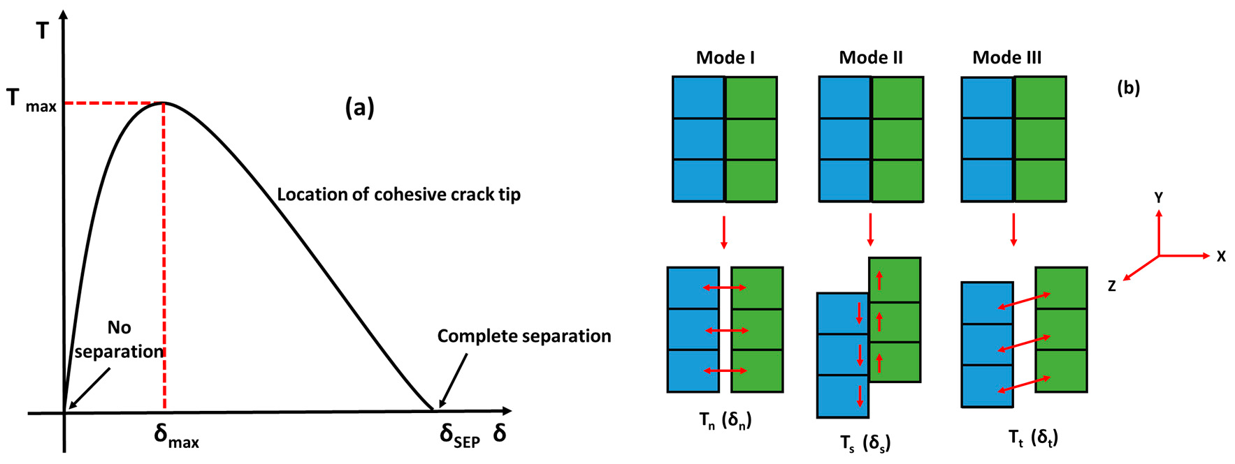
A bilinear cohesive law is implemented in this work (see Equation (1)), which reduces the artificial compliance inherent in CZM. Figure 1 illustrates the various stages of cohesive zone damage. is the average interfacial shear stress and δ is the relative tangential displacement. The traction across the interface increases and reaches a peak value, and then decreases and eventually vanishes, resulting in a complete decohesion, given by Equation (1).
Commercial finite element code (Abaqus Version 6.13) was used to model the cohesive zone in the fiber/interface debonding and/or pull-out. The relation between traction stress and separation is given by Equation (2),
where Tn is the traction stress in the normal direction, Ts, Tt are traction stresses in the first shear and the second shear directions, respectively, K is the normal stiffness matrix, and δn, δs, and δt are separations in the normal, first, and second shear directions, respectively. The elastic stiffness and the cohesive strength would be obtained from experiments. The maximum stress criteria were used to predict damage initiation, given by Equation (3).
signify the peak values for traction stresses in the respective directions. Damage evolution law describes the rate at which the cohesive stiffness is degraded once the corresponding initiation criteria is reached. A scalar damage variable, D, represents the overall damage at the contact point, which is represented below. The value of D ranges from 0 to 1. Refer to Equation (4).
CZM was used to predict the initiation and evolution of damage at the interface of the unit cell comprising the fiber and matrix. For a composite unit cell that consists of multiple material systems, the number of potential failure mechanisms that must be accounted for exponentially increases the complexity of the analysis. Failure mechanisms include failure at the interface, fiber breakage, matrix cracking, and their interaction.
Different modeling approaches within CZM were employed, such as elements with ‘zero thickness’ and ‘finite thickness’—(a) the interface was modeled as ‘zero thickness’ and adhesive properties were used to study the interface failure mechanism; and (b) the interface was modeled with a very small thickness for the ‘finite thickness model,’ respectively. Parametric studies were also conducted to study the most influential factors affecting the strength of the fiber matrix unit cell.
3. Finite Element Model Setup
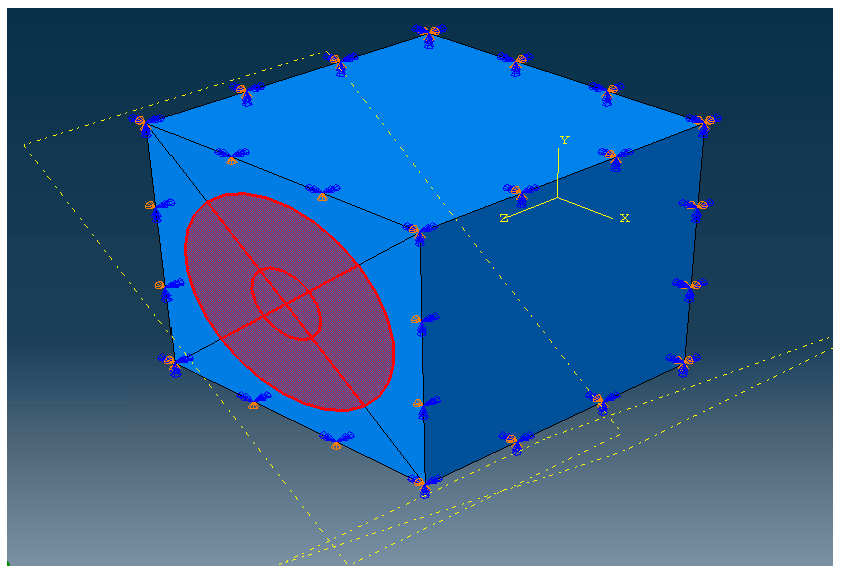
A 3D finite element model of the fiber pull-out specimen was generated using the CZM approach. The finite element model of the unit cell and the boundary conditions are shown in Figure 2. The radius of the fiber was 7.5 µm and the fiber was encased in a square matrix that was 18.8 µm. The dimension of the matrix was based on a fiber volume fraction of 60%.
Both the fiber and the matrix were modeled using 3D first-order (linear) hexahedron elements with incompatible modes (C3D8I) in Abaqus, which is an improved version of the C3D8 element. The boundary conditions that are constraints are also shown in Figure 2. More details about this type of element are available from [14].
The interface was modeled with zero thickness. In this model, the Young’s modulus value for the interface was assumed to be equal to the matrix properties. However, the interfacial shear strength or the strength of the interface was taken from [16], which is 25 MPa. This value was measured by a single-fiber fragmentation test wherein a single fiber was embedded in an epoxy matrix by Kumar [16] who studied the effect of sizing on interfacial strength properties.
The material and input parameters are summarized in Table 1. The contact behavior of the fiber/matrix interface was modeled as discussed in Section 2 using surface-based cohesive behavior, which is similar to the cohesive element approach. This is a preferred approach when the interface or the adhesive layer is very thin [14]. A displacement-controlled load of 0.1 mm was applied at the free end of the fiber. The reason for imposing displacement on the fiber was that it results in a more gradual failure process than a similar loading using applied forces [17]. A similar approach was used by Bhemareddy et al. in Ref. [18] in their finite element model for the debonding of a silicon carbide fiber (SiCf) embedded in a silicon carbide matrix (SiC).
4. Results and Discussion
4.1. Effect of Continuous and Discontinuous Bonding between the Fiber and Matrix
Two cases were studied with this model to understand the effect of sizing coverage on the fiber. In one case, the complete surface of the fiber is bonded to the matrix while, in the second case, only half the surface of the fiber is bonded to the matrix. This simulates the situation where only half of the fiber has been coated with sizing while the other half is uncoated. This is very close to the real-life situation wherein a typical sizing applicator operates on at least two bundles of fibers. Each bundle of fibers travels from a bushing above this applicator down to a winder below [19]. Due to the nature of this process, uneven sizing is deposited on the fiber surface.
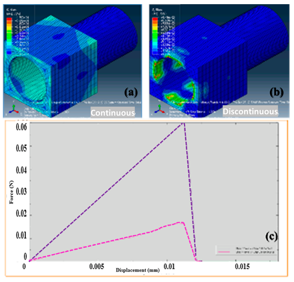
The stresses on the matrix region for discontinuous coating (shown in Figure 3b) are one magnitude lower than those for continuous coating (Figure 3a). This can be attributed to the fact that less force is required in the case of discontinuous coating. The force required to pull-out the fiber from the matrix for the continuous coating model was 0.06 N, while it was only 0.015 N for discontinuous coating, as shown in Figure 3c.
The 3D finite element model simulates the situation when only half of the fiber is bonded to the matrix, and it has the potential of near-accurately predicting the load-displacement behavior when a single fiber is debonded from an encased matrix.
4.2. Parametric Study to Understand Influential Factors in Fiber Matrix Adhesion
A parametric study was undertaken on a 2D axisymmetric model to understand the influential factors affecting the fiber-matrix adhesion. Load-displacement behavior predicted by changes in these factors were recorded and compared to each other. The radius of the fiber was 7.5 µm and that of the matrix was 1.5 mm. Both the fiber and the matrix were modeled using four-node bilinear axisymmetric quadrilateral elements with reduced integration (CAX4R). CZM was used for this model. A displacement-controlled load of 0.1 mm is applied on the free end of the fiber. The factors studied are: (a) Coefficient of friction (static and dynamic), (b) cohesive stiffness of the interface, (c) cohesive strength of the interface, (d) fiber embedded length.
4.3. Effect of Coefficient of Friction
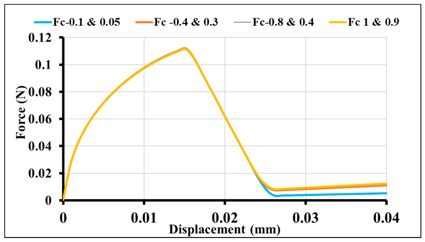
The parameter-coefficient of friction primarily comes into play only after complete debonding has taken place. Figure 4 shows the load-displacement plots for the finite element models with varying coefficients of friction. Four different sets of static and dynamic coefficients of friction were used in the parametric study. They were: (0.1 and 0.05), (0.4 and 0.3), (0.8 and 0.4), and (1 and 0.9).
Figure 4 is a magnified version and, hence, the non-linearity of the force-displacement curve is exaggerated. However, the nature of the curve is non-linear to an extent and is not representative of an actual test. This could be due to the effects of coefficients of thermal expansion and residual stresses on the fiber, which have not been accounted for in this model. Nevertheless, finite element models generated by various researchers [4,20,21] have the same trends associated with the force-displacement curve.
4.4. Effect of Cohesive Stiffness of the Interface
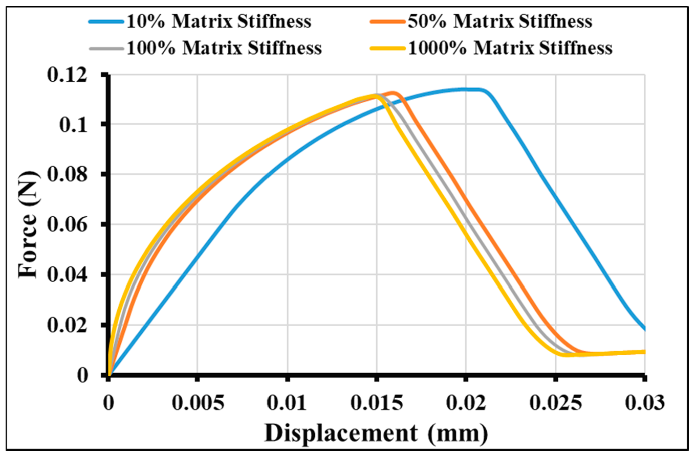
The elastic modulus/stiffness of the interface was provided as an input property in the cohesive behavior for the interface in Abaqus. The basic assumption here was that the interface would behave similar to that of the matrix; hence, properties of the epoxy matrix were considered as the baseline. The interface stiffness was varied from 10% of the matrix stiffness to 1000% of the matrix stiffness in discrete values as 10%, 50%, 100%, and 1000% respectively.
As reported in Table 2, the elastic modulus for the epoxy matrix and the interface was taken to be 4200 MPa. Figure 5 shows the load-displacement behavior for varying moduli of the interface. It was noticed that the peak force required for debonding does not change even when the modulus of the interface is as low as 420 MPa. In addition, the higher the stiffness of the interface, the lower the displacement (complete separation). Furthermore, it was seen that for a very low interface modulus (420 MPa), the evolution of crack length was much higher when compared to other cases. This is along expected lines as the interface is too weak.
4.5. Effect of Cohesive Strength of the Interface
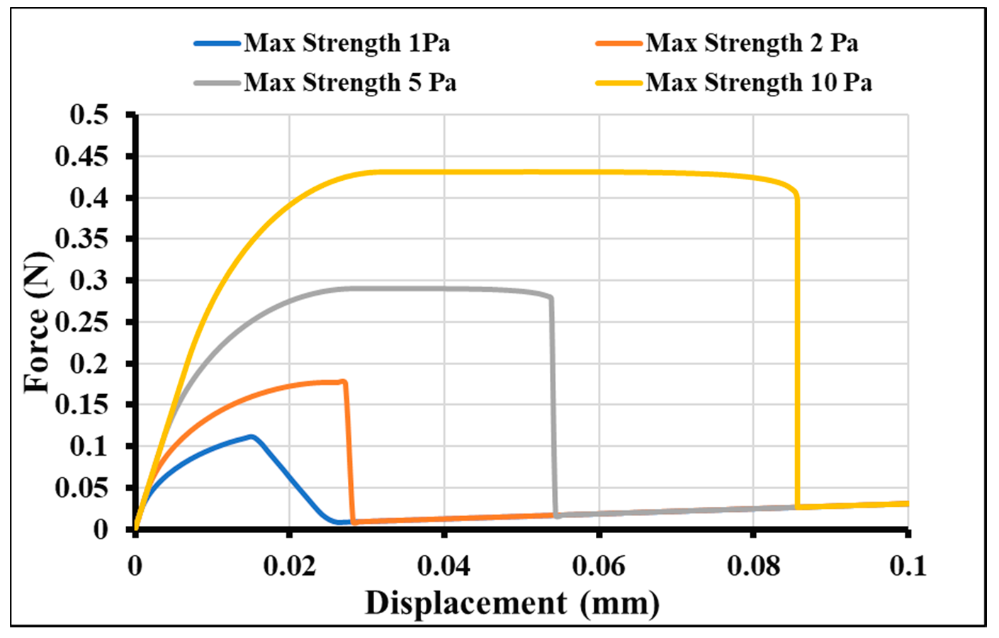
The strength of the interface was varied starting from 1 to 10 MPa, keeping all the other variables at the baseline configurations. It can be clearly seen from Figure 6 that interfacial strength would directly affect the maximum load at which the interface fails. The peak load is almost proportional to the strength of the interface. It is also worth noting that at higher strength, ductile behavior of the interface is seen. In other words, the crack has initiated but, as the bond strength is too high, the crack evolution does not take place and debonding is delayed.
4.6. Effect of Embedded Fiber Length
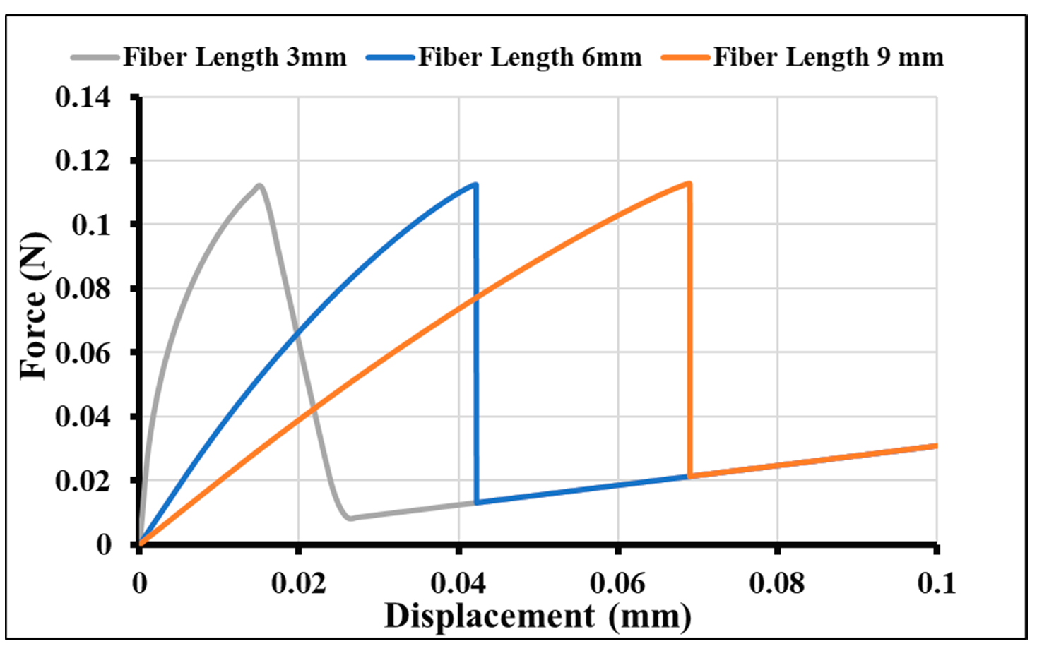
The effect of fiber-embedded length is more pronounced in terms of the maximum separation achieved. Three different fiber lengths (3, 6, and 9 mm) were used in the parametric study, and the respective load-displacement curves are illustrated in Figure 7. As the fiber length increased, it was observed that the fiber-matrix response became more compliant and delayed debonding was observed.
A similar observation was observed by Sockalingam et al. [22] when they developed a finite element model of the micro-droplet test method. The micro-droplet test is one of the best techniques to study the interfacial properties between a fiber and matrix. This can be attributed to the fact that the fiber bears the load when it is pulled out of the matrix.
4.7. Stress Distribution at Debonding between the Fiber, Interface, and the Matrix
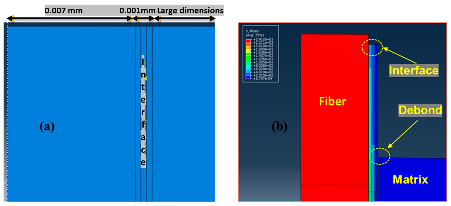
Shear stress distribution across the interface during the debonding stage is an important indicator of the interface and adhesion within the fiber/matrix. To investigate this effect, a 2-D axisymmetric model was created where the interface was given a thickness of 0.001 mm, the fiber diameter was 0.007 mm, and the matrix was 1.5 mm. This is shown in Figure 8. Furthermore, the interface was divided into three sections and each had its own isotropic material property assigned. The three sections were: (a) Interface close to the fiber, which was assigned fiber property; (b) interface in the middle, which was assigned the average constituent fiber and resin property; and (c) interface closer to the resin, which was matrix-dominated. The representation of the model is shown in Figure 8. Details of the input properties used in Abaqus are provided in Table 3. The assumption for the interface was that it would behave like a glass fiber when near the fiber and similar to the resin when in contact with the resin. CZM was employed here as well when considering the bond between the interface, fiber, and matrix.
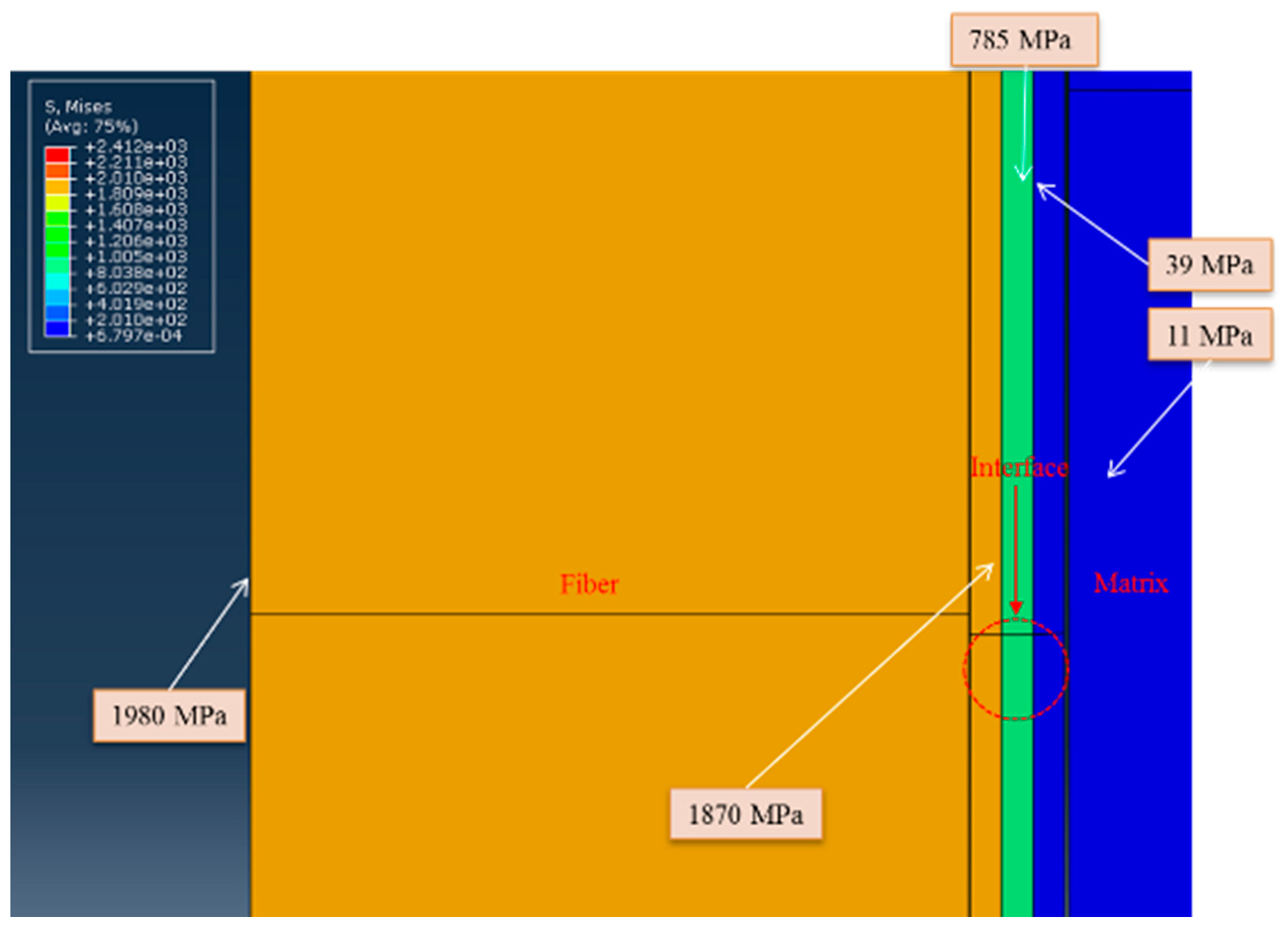
A pressure load was applied on the free end of the fiber, and the shear stress distribution across the fiber, interface, and the matrix was recorded. The boundary condition was applied to mimic a fiber pull-out where the bottom part of the matrix block is fixed and the fiber is pulled from the top end. Symmetry about the axis is also considered as it is an axisymmetric model. As higher strength was provided at the fiber-interface zone (Modulus 50 GPa), it was observed that debonding does not take place in this zone. However, the debonding occurs in the interface-matrix region (3.5 GPa). Figure 8 shows the shear stress distribution across the model. This was based on an assumption that the interface takes the property of the fiber in this zone, and the interface fails mostly in the matrix region, if the interface itself is not the weakest link.
The 2D axisymmetric model covers the entire range of intricacies involved in adhesion of the fiber and the interface and the matrix. It was observed that the interface, which was modeled as a thin film between the fiber and the matrix, continued to remain bonded with the fiber. Figure 9 shows a stress contour plot of all three sections of the model. As discussed above, the stress is mostly borne by the fiber and then then reduces gradually. The stresses calculated were 1980, 1870, 785, 39, and 11 MPa for the fiber, fiber-dominated interface, average interface, resin-dominated interface, and the matrix, respectively.
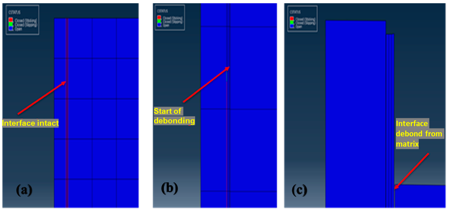
The CONTACT STATUS (CSTATUS) feature of Abaqus was used throughout the analysis between the bonded surfaces. It is divided into three parts—‘stick, slip, and open.’ The CSTATUS provides an indication (a) when the contact is closed and is intact; (b) when it has begun degrading; and (c) when it is completely open. Figure 10 illustrates the contact status at various stages of the analysis. At the initial stage, the contact is entirely intact between both the surfaces; in the middle stage of the analysis, progressive debonding takes place between the interface-matrix zones.
5. Discussion
With the application of CZM, the finite element models demonstrate a single-fiber pull-out process very well. Even though the finite element models developed herein were for glass fibers, the same methodology can also be employed for carbon fibers. The parameters that would change are—radius of the fiber, dimension of the matrix block, friction coefficient, and interfacial crack initiation shear stress. More details on modeling parameters can be found in [23]. In Ref. [23], the authors have followed the CZM approach and simulated a single-carbon-fiber pull-out using the commercial finite element package Abaqus.
The finite element models in the current study have shown good potential to predict the load-displacement behavior. Availability of more data sets from exhaustive tests would make the model more robust and could be used for further investigation of adhesion between the fiber, interface, and matrix. The finite element models need to be validated by comparing to experimental test results, and they can be improved further to predict the load-displacement interfacial behavior during fiber-pull out.
Having analyzed the fiber/matrix interface using both 3-D models and 2-D models, it is clear that both the approaches have their advantages with respect to each other; however, the 2-D axisymmetric model with its relatively simple and user-friendly approach coupled with lower computational time was preferred. As both the models (3D and 2D) follow the same principles of CZM, the fundamentals remain the same.
6. Conclusions
This study addressed the interfacial characteristics in fiber-reinforced composites. A 2D and 3D finite element model of the fiber pull-out specimen was generated using the CZM approach. The key findings from the modeling were: (a) The effect of sizing coverage was found to be pronounced. While the force required to pull-out the fiber from the matrix for the continuous coating model was 0.06 N, it was only 0.015 N for discontinuous coating, a 300% increase with uniform sizing coverage; (b) The static and dynamic coefficient of friction had a moderate effect on the force-displacement past debonding of the interface. Friction coefficients greater than 0.3 resulted in about a 66% higher interface force magnitude over lower values of friction coefficients; (c) for varying degrees of interface stiffness ranging from 10% to 1000% of the matrix stiffness (modulus), it was noticed that the peak force required for debonding does not change even for 10% of the matrix stiffness. In addition, the higher the stiffness of the interface, the lower the displacement (complete separation); (d) varying the interface strength from 1 to 10 MPa directly affected the maximum load at which the interface fails. The peak load is proportional to the strength of the interface; (e) in terms of embedded fiber length, as the fiber length increased, it was observed that the fiber-matrix interface becomes more compliant and delays debonding; and (f) for the high-fiber-interface zone (for example, modulus 50 GPa), it was observed that the debond does not take place in this zone, but the debond takes place in the interface-matrix region (for example, modulus 3.5 GPa). With larger data sets available from experimental results in the future, these models can be used to capture details that are otherwise difficult to study. Furthermore, the findings from this study can be used in the composites industry to characterize and evaluate different fiber surfaces.
Author Contributions
Conceptualization, U.V., A.V.; methodology, D.K.S., V.T.; software, D.K.S.; validation, A.V., S.K., M.T.; formal analysis, D.K.S., S.K.; investigation, D.K.S.; resources, A.V., M.T.; data curation, D.K.S., S.K.; writing—original draft preparation, D.K.S., U.V.; writing—review and editing, U.V., A.V., V.T.; visualization, D.K.S.; supervision, U.V., A.V.; project administration, U.V.; funding acquisition, U.V., A.V. All authors have read and agreed to the published version of the manuscript.
Funding
This research was funded by US Department of Energy (DOE) Graduate Automotive Technology Education (GATE) Owens Corning (OC) and Institute for Advanced Composites Manufacturing Innovation (IACMI)-The Composites Institute. The information, data, and work presented herein were funded in part by the US Department of Energy (DOE), Office of Energy Efficiency and Renewable Energy, under Award Number DE-EE0006926 and in part by US DOE GATE DE-FG26-05NT42620.
Conflicts of Interest
The authors declare no conflict of interest.
References
- Mallick, P.K. Fiber-Reinforced Composites: Materials, Manufacturing, and Design; CRC Press: Boca Raton, FL, USA, 2010. [Google Scholar]
- Drzal, L. TheInterphase in Epoxy Composites. In Epoxy Resins and Composites; Dušek, K., II, Ed.; Springer: Berlin/Heidelberg, Germany, 1986; pp. 1–32. [Google Scholar]
- Pitkethly, M.; Favre, J.; Gaur, U.; Jakubowski, J.; Mudrich, S.F.; Caldwell, D.L.; Lawrence, T. A Round-Robin Programme on Interfacial Test Methods. Compos. Sci. Technol. 1993, 48, 205–214. [Google Scholar] [CrossRef]
- Sockalingam, S.; Nilakantan, G. Fiber-Matrix Interface Characterization Through the Microbond Test. Int. J. Aeronaut. Space Sci. 2012, 13, 282–295. [Google Scholar] [CrossRef] [Green Version]
- Gaur, U.; Miller, B. Microbond Method for Determination of the Shear Strength of a Fiber/Resin Interface: Evaluation of Experimental Parameters. Compos. Sci. Technol. 1989, 34, 35–51. [Google Scholar] [CrossRef]
- Hsueh, C.-H. Interfacial Debonding and Fiber Pull-out Stresses of Fiber-Reinforced Composites. Mater. Sci. Eng. 1990, 123, 1–11. [Google Scholar] [CrossRef]
- Stang, H.; Shah, S.P. Failure of Fibre-Reinforced Composites by Pull-out Fracture. J. Mater. Sci. 1986, 21, 953–957. [Google Scholar] [CrossRef]
- Gao, Y.-C.; Mai, Y.-W.; Cotterell, B. Fracture of Fiber-Reinforced Materials. Z. für angewandte Mathematik und Physik ZAMP 1988, 39, 550–572. [Google Scholar] [CrossRef]
- Sun, W.; Lin, F. Computer Modeling and FEA Simulation for Composite Single Fiber pull-out. J. Thermoplast. Compos. Mater. 2001, 14, 327–343. [Google Scholar] [CrossRef]
- Wei, G.F.; Liu, G.Y.; Xu, C.H.; Sun, X.Q. Finite Element Simulation of Perfect Bonding for Single Fiber pull-out Test. Adv. Mater. Res. 2012, 418, 509–512. [Google Scholar] [CrossRef]
- Dugdale, D.S. Yielding of Steel Sheets Containing Slits. J. Mech. Phys. Solids 1960, 8, 100–104. [Google Scholar] [CrossRef]
- Barenblatt, G.I. The Mathematical Theory of Equilibrium of Crack in Brittle Fracture. Adv. Appl. Mech. 1962, 7, 55–129. [Google Scholar]
- Chandra, N. Evaluation of Interfacial Fracture Toughness Using Cohesive Zone Model. Compo. Part A Appl. Sci. Manuf. 2002, 33, 1433–1447. [Google Scholar] [CrossRef]
- Hibbit, K.; Sorensen, A. Abaqus Standard Analysis User’s Manual; Hibbit, Karlsson, Sorensen Inc.: Providence, RI, USA, 2007. [Google Scholar]
- Cornec, A.; Scheider, I.; Schwalbe, K.-H. On the Practical Application of the Cohesive model. Eng. Fract. Mech. 2003, 70, 1963–1987. [Google Scholar] [CrossRef]
- Kumar, G.K. Studying the Influence of Glass Fiber Sizing Roughness and Thickness with the Single Fiber Fragmentation Test; Degree Project; Kristianstad University: Kristianstad, Sweden, 2006. [Google Scholar]
- Firehole Technologies. Helius: MCT Tutorial 1; Firehole Technologies: Laramie, WY, USA, 2011. [Google Scholar]
- Venkata Bheemreddy, K. Chandrashekhara, Lokeswarappa R. Dharani, Greg Eugene Hilmas, Modeling of Fiber pull-out in Continuous Fiber Reinforced Ceramic Composites Using Finite Element Method and Artificial Neural Networks. Comput. Mater. Sci. 2013, 79, 663–673. [Google Scholar] [CrossRef]
- Mason, K. Sizing up Fiber Sizings. 2006. Available online: http://www.compositesworld.com/articles/sizing-up-fiber-sizings (accessed on 6 September 2012).
- Gao, X.; Jensen, R.; McKnight, S.; Gillespie, J., Jr. Effect of Colloidal Silica on the Strength and Energy Absorption of Glass Fiber/Epoxy Interphases. Compos. Part A Appl. Sci. Manuf. 2011, 42, 1738–1747. [Google Scholar] [CrossRef]
- Scheer, R.; Nairn, J. A Comparison of Several Fracture Mechanics Methods for Measuring Interfacial Toughness with Microbond Tests. J. Adhes. 1995, 53, 45–68. [Google Scholar] [CrossRef]
- Sockalingam, S.; Dey, M.; Gillespie, J.W., Jr.; Keefe, M. Finite Element Analysis of the Microdroplet Test Method Using Cohesive Zone Model of the Fiber/Matrix Interface. Compos. Part A Appl. Sci. Manuf. 2014, 56, 239–247. [Google Scholar] [CrossRef]
- Jia, Y.; Yan, W.; Liu, H.-Y. Numerical study on carbon fibre pullout using a cohesive zone model. In Proceedings of the 18th International Conference on Composite Materials, Jeju Island, Korea, 21–26 August 2011. [Google Scholar]
Figure 1.
Cohesive zone damage; (a) typical traction separation behavior when a fiber is pulled out from the matrix [14], (b) traction separations for different fracture modes. Mode II fracture mode has been used in this analysis [15].

Figure 2.
3-D unit cell model where the purple circle indicates the fiber and the square represents the matrix within which the fiber is enclosed. The boundary conditions are also shown here.
Figure 2.
3-D unit cell model where the purple circle indicates the fiber and the square represents the matrix within which the fiber is enclosed. The boundary conditions are also shown here.

Figure 3.
(a) Stress plot for continuous interface coating on the fiber, (b) stress plot for discontinuous interface coating on the fiber, and (c) force-displacement plot for the simulated fiber pull-out where force is measured in (N) and displacement in (mm).
Figure 3.
(a) Stress plot for continuous interface coating on the fiber, (b) stress plot for discontinuous interface coating on the fiber, and (c) force-displacement plot for the simulated fiber pull-out where force is measured in (N) and displacement in (mm).

Figure 4.
Force (or load)-displacement curve for varying coefficients of friction.

Figure 5.
Force-displacement curve for varying interface stiffness.

Figure 6.
Force-displacement curve for varying cohesive strength.

Figure 7.
Force-displacement curve for varying fiber length.

Figure 8.
Shear stress distribution across the constituents—(a) dimension of the unit cell model, (b) debond stage. The stress contour plot is also seen here.
Figure 8.
Shear stress distribution across the constituents—(a) dimension of the unit cell model, (b) debond stage. The stress contour plot is also seen here.

Figure 9.
Stress values calculated during the simulation for each section (fiber, interface, and the matrix).
Figure 9.
Stress values calculated during the simulation for each section (fiber, interface, and the matrix).

Figure 10.
Finite element modeling of fiber pull-out and debonding: (a) Represents initial stage of pull-out where the red part indicates the interface is intact, (b) represents the middle stage of simulation where the absence of red spots indicates debonding, and (c) represents the debond between the matrix and interface.


Table 1.
Material properties used in the 3D finite element model.
| Material | Modulus (GPa) | Tensile Strength (MPa) | Coefficient of Friction (Static and Dynamic) | Poisson’s Ratio |
|---|---|---|---|---|
| E-Glass Fiber | 72 | - | - | 0.2 |
| Epoxy Matrix | 4.2 | - | - | 0.34 |
| Interface (Cohesive Zone) | 4.2 | 25 | 1 and 0.9 | - |
Table 2.
Baseline material properties used in 2D axisymmetric model.
| Material | Modulus (GPa) | Tensile Strength (MPa) | Coefficient of Friction (Static and Dynamic) | Poisson’s Ratio |
|---|---|---|---|---|
| E-Glass Fiber | 72 | - | - | 0.2 |
| Epoxy Matrix | 4.2 | - | - | 0.34 |
| Interface (Cohesive Zone) | 4.2 | 25 | 1 and 0.9 | - |
Table 3.
Input properties for three-phase model where interface is modeled as a separate entity.
| Material | Modulus (GPa) | Tensile Strength (MPa) | Poisson’s Ratio |
|---|---|---|---|
| E-CR-glass | 81 | - | 0.2 |
| Epoxy Matrix | 4.2 | - | 0.3 |
| Interface (Fiber-Dominated) | 4.2 | - | - |
| Interface (Fiber/resin Average) | 42.6 | - | 0.3 |
| Interface (Resin-Dominated) | 4.2 | - | 0.3 |
| Fiber-Interface (Cohesive Zone) | 50 | 40 | - |
| Matrix-Interface (Cohesive Zone) | 3.5 | 10 | - |
© 2020 by the authors. Licensee MDPI, Basel, Switzerland. This article is an open access article distributed under the terms and conditions of the Creative Commons Attribution (CC BY) license (http://creativecommons.org/licenses/by/4.0/).
Share and Cite
MDPI and ACS Style
Singh, D.K.; Vaidya, A.; Thomas, V.; Theodore, M.; Kore, S.; Vaidya, U. Finite Element Modeling of the Fiber-Matrix Interface in Polymer Composites. J. Compos. Sci. 2020, 4, 58. https://0-doi-org.brum.beds.ac.uk/10.3390/jcs4020058
AMA Style
Singh DK, Vaidya A, Thomas V, Theodore M, Kore S, Vaidya U. Finite Element Modeling of the Fiber-Matrix Interface in Polymer Composites. Journal of Composites Science. 2020; 4(2):58. https://0-doi-org.brum.beds.ac.uk/10.3390/jcs4020058
Chicago/Turabian StyleSingh, Daljeet K., Amol Vaidya, Vinoy Thomas, Merlin Theodore, Surbhi Kore, and Uday Vaidya. 2020. "Finite Element Modeling of the Fiber-Matrix Interface in Polymer Composites" Journal of Composites Science 4, no. 2: 58. https://0-doi-org.brum.beds.ac.uk/10.3390/jcs4020058